0306E - Faculty of Social Sciences - Université d'Ottawa

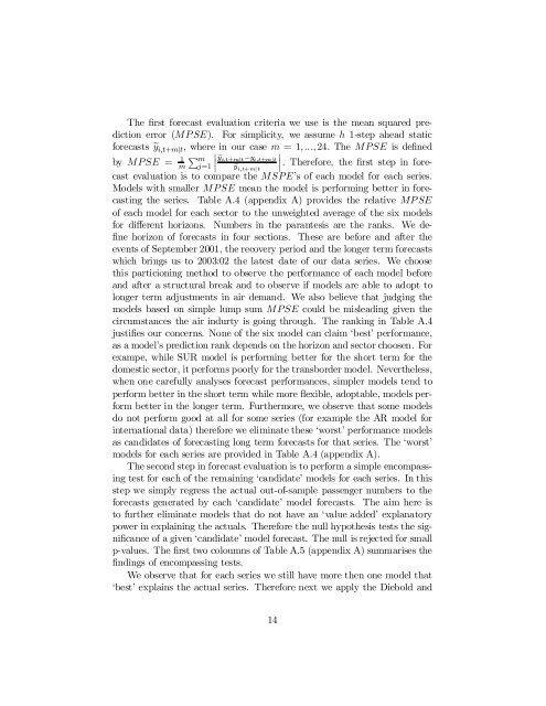
The …rst forecast evaluation criteria we use is the mean squared prediction
error (MP SE). For simplicity, we assume h 1-step ahead static
forecasts ey i;t+mjt ; where in our case m = 1; :::; 24: The MPSE is de…ned
by MPSE =
m 1 P mj=1 ey
¯¯¯
i;t+mjt ¡y i;t+mjt
ey i;t+mjt
¯¯¯ : Therefore, the …rst step in forecast
evaluation is to compare the MSPE’s of each model for each series.
Models with smaller MPSE mean the model is performing better in forecasting
the series. Table A.4 (appendix A) provides the relative MP SE
of each model for each sector to the unweighted average of the six models
for di¤erent horizons. Numbers in the parantesis are the ranks. We de-
…ne horizon of forecasts in four sections. These are before and after the
events of September 2001, the recovery period and the longer term forecasts
which brings us to 2003:02 the latest date of our data series. We choose
this particioning method to observe the performance of each model before
and after a structural break and to observe if models are able to adopt to
longer term adjustments in air demand. We also believe that judging the
models based on simple lump sum MPSE could be misleading given the
circumstances the air indurty is going through. The ranking in Table A.4
justi…es our concerns. None of the six model can claim ‘best’ performance,
as a model’s prediction rank depends on the horizon and sector choosen. For
exampe, while SUR model is performing better for the short term for the
domestic sector, it performs poorly for the transborder model. Nevertheless,
when one carefully analyses forecast performances, simpler models tend to
perform better in the short term while more ‡exible, adoptable, models perform
better in the longer term. Furthermore, we observe that some models
do not perform good at all for some series (for example the AR model for
international data) therefore we eliminate these ‘worst’ performance models
as candidates of forecasting long term forecasts for that series. The ‘worst’
models for each series are provided in Table A.4 (appendix A).
The second step in forecast evaluation is to perform a simple encompassing
test for each of the remaining ‘candidate’ models for each series. In this
step we simply regress the actual out-of-sample passenger numbers to the
forecasts generated by each ‘candidate’ model forecasts. The aim here is
to further eliminate models that do not have an ‘value added’ explanatory
power in explaining the actuals. Therefore the null hypothesis tests the signi…cance
of a given ‘candidate’ model forecast. The null is rejected for small
p-values. The …rst two coloumns of Table A.5 (appendix A) summarises the
…ndings of encompassing tests.
We observe that for each series we still have more then one model that
‘best’ explains the actual series. Therefore next we apply the Diebold and
14