Rate Adaptation in Time Varying Channels using Acknowledgement ...

Rate Adaptation in Time Varying Channels using
Acknowledgement Feedback
Chin Keong Ho
Eindhoven University of Technology
PO Box 513, 5600 MB Eindhoven
The Netherlands
Email: c.k.ho@tue.nl
Job Oostveen
Philips Research Laboratories
Prof. Holstlaan 4, 5656 AA Eindhoven
The Netherlands
Email: job.oostveen@philips.com
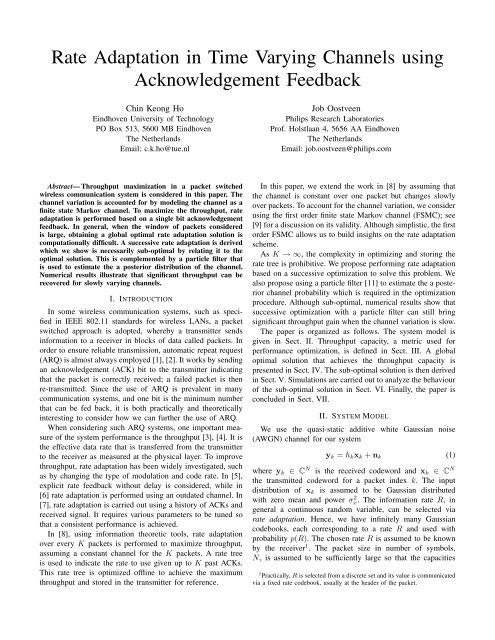
Abstract— Throughput maximization in a packet switched
wireless communication system is considered in this paper. The
channel variation is accounted for by modeling the channel as a
finite state Markov channel. To maximize the throughput, rate
adaptation is performed based on a single bit acknowledgement
feedback. In general, when the window of packets considered
is large, obtaining a global optimal rate adaptation solution is
computationally difficult. A successive rate adaptation is derived
which we show is necessarily sub-optimal by relating it to the
optimal solution. This is complemented by a particle filter that
is used to estimate the a posterior distribution of the channel.
Numerical results illustrate that significant throughput can be
recovered for slowly varying channels.
I. INTRODUCTION
In some wireless communication systems, such as specified
in IEEE 802.11 standards for wireless LANs, a packet
switched approach is adopted, whereby a transmitter sends
information to a receiver in blocks of data called packets. In
order to ensure reliable transmission, automatic repeat request
(ARQ) is almost always employed [1], [2]. It works by sending
an acknowledgement (ACK) bit to the transmitter indicating
that the packet is correctly received; a failed packet is then
re-transmitted. Since the use of ARQ is prevalent in many
communication systems, and one bit is the minimum number
that can be fed back, it is both practically and theoretically
interesting to consider how we can further the use of ARQ.
When considering such ARQ systems, one important measure
of the system performance is the throughput [3], [4]. It is
the effective data rate that is transferred from the transmitter
to the receiver as measured at the physical layer. To improve
throughput, rate adaptation has been widely investigated, such
as by changing the type of modulation and code rate. In [5],
explicit rate feedback without delay is considered, while in
[6] rate adaptation is performed using an outdated channel. In
[7], rate adaptation is carried out using a history of ACKs and
received signal. It requires various parameters to be tuned so
that a consistent performance is achieved.
In [8], using information theoretic tools, rate adaptation
over every K packets is performed to maximize throughput,
assuming a constant channel for the K packets. A rate tree
is used to indicate the rate to use given up to K past ACKs.
This rate tree is optimized offline to achieve the maximum
throughput and stored in the transmitter for reference.
In this paper, we extend the work in [8] by assuming that
the channel is constant over one packet but changes slowly
over packets. To account for the channel variation, we consider
using the first order finite state Markov channel (FSMC); see
[9] for a discussion on its validity. Although simplistic, the first
order FSMC allows us to build insights on the rate adaptation
scheme.
As K →∞, the complexity in optimizing and storing the
rate tree is prohibitive. We propose performing rate adaptation
based on a successive optimization to solve this problem. We
also propose using a particle filter [11] to estimate the a posterior
channel probability which is required in the optimization
procedure. Although sub-optimal, numerical results show that
successive optimization with a particle filter can still bring
significant throughput gain when the channel variation is slow.
The paper is organized as follows. The system model is
given in Sect. II. Throughput capacity, a metric used for
performance optimization, is defined in Sect. III. A global
optimal solution that achieves the throughput capacity is
presented in Sect. IV. The sub-optimal solution is then derived
in Sect. V. Simulations are carried out to analyze the behaviour
of the sub-optimal solution in Sect. VI. Finally, the paper is
concluded in Sect. VII.
II. SYSTEM MODEL
We use the quasi-static additive white Gaussian noise
(AWGN) channel for our system
y k = h k x k + n k (1)
where y k ∈ C N is the received codeword and x k ∈ C N
the transmitted codeword for a packet index k. The input
distribution of x k is assumed to be Gaussian distributed
with zero mean and power σx. 2 The information rate R, in
general a continuous random variable, can be selected via
rate adaptation. Hence, we have infinitely many Gaussian
codebooks, each corresponding to a rate R and used with
probability p(R). The chosen rate R is assumed to be known
by the receiver 1 . The packet size in number of symbols,
N, is assumed to be sufficiently large so that the capacities
1 Practically, R is selected from a discrete set and its value is communicated
via a fixed rate codebook, usually at the header of the packet.

and information outages defined throughout this paper are
achievable. The complex channel h k , with variance σh 2 , is time
invariant for each packet but varies across packets. The noise
vector n k ∈ C N is AWGN with variance σn.
2
If a packet is not received correctly, an outage is said
to occur. Practically, this information is available at the receiver
via a cyclic redundancy check (CRC) at the medium
access control (MAC) layer. The packet is either discarded
or re-transmitted later in non-delay sensitive applications.
The present packet therefore fails to deliver the data bits
and the instantaneous throughput is zero. Otherwise, if the
packet is received correctly, the instantaneous throughput, in
bit/symbols, equals the data rate. The throughput for the k th
packet is therefore defined as
T (¯γ,R k ,h k )=R k × (1 − ɛ(¯γ|R k ,h k )) (2)
where ɛ(¯γ|R k ,h k ) is the outage probability at an average SNR
¯γ = σ 2 h σ2 x/σ 2 n for a given R k and h k . The actual outage
probability function depends on the error correction code used.
We treat every K packets as one basic unit: a K-packet.
The throughput of a K-packet system with average SNR ¯γ
can be generally defined as
T K (¯γ,r K , h K )= 1 K
K∑
T (¯γ,R k ,h k ) (3)
k=1
where h K =[h 1 h 2 ···h K ] and the rate vector is given by
r K =[R 1 R 2 ···R K ].TherateR k determines the throughput
of packet k as reflected in (3). Interesting, the rate also affects
the ability of the transmitter to observe the channel, or CSI,
via the ACK feedback - this will become apparent in the next
section.
III. THROUGHPUT CAPACITY
A. Full Channel State Information (CSI)
We are interested in maximizing the average throughput
of (3) using a packet-by-packet rate adaption scheme. The
throughput capacity, or the maximum throughput achievable
over the joint distribution of the rate and channel, is defined
as
CT K [
,full CSI(¯γ) = sup E rK,h K T K (¯γ,r K , h K ) ]
p(r K,h K)
[
= sup E rK,h K T K (¯γ,r K , h K ) ] (4)
p(r K|h K)
where E is the expectation operator (over the distribution
given by its subscript). Here, for full generality, we assume
that the rate is a random variable for which we want to
find the optimal distribution. The second line follows since
p(r K , h K )=p(r K |h K )p(h K ) and p(h K ) is related to the
channel and is not a parameter available for maximization. It
turns out that to achieve the throughput capacity without any
restriction, full CSI via h K is required at the transmitter.
In practice, full CSI is not available, and also there is a
delay in obtaining the CSI. A more general definition for the
case that a partial CSI is known at the transmitter follows.
B. Partial CSI
In general, we want to maximize the throughput using rate
adaption given a partial channel knowledge expressed as a
random parameter a (which can be discrete or continuous,
scalar or vector). The distribution available for maximization
is therefore restricted to p(r K |a). However, we now need to
take into account the extra random variable a in performing
the expectation in (4). This gives us the throughput capacity
CT K [
(¯γ) = sup E rK,h K,a T K (¯γ,r K , h K ) ] . (5)
p(r K|a)
This formulation reduces to (4) when a = h K . The case when
no channel knowledge is available can be treated by letting a
be an empty vector in (5). The special case when the channel
is constant over K packets can be treated by setting h k = h
for all k, which is considered in [8].
We now consider the case of interest here in using (5). In
the MAC protocol, the simplest feedback provided is via a
ACK or negative ACK, i.e. NACK. This is a form of partial
CSI. Specifically, denote the CSI of packet k as A k with value
1 for ACK and 0 for NACK. Their probabilities are
p(A k =1|R k ,h k )=1− ɛ(¯γ|R k ,h k ), (6)
p(A k =0|R k ,h k )=ɛ(¯γ|R k ,h k ). (7)
Obviously, A k is dependent on R k , since if R k is large, the
possibility of A k =0is high. For the ARQ system, we can
replace a in (5) by the ACK vector a K−1 , where we denote
a k−1 [a k−2 ,A k−1 ],k = 2, 3, ··· , and a 0 is an empty
vector.
On the other hand, not all of the ACKs and rates are always
available for rate adaptation due to a causality constraint. The
information available at packet k is only a k−1 and r k−1 .Tobe
exact, R k should then be written explicitly as 2 R k (a k−1 , r k−1 )
when substituting (3) into (5). Similarly, the rate vector should
be understood as dependent on the the past ACKs and rates,
in the form of r k (a k−1 , r k−1 ). However, the argument will be
dropped when there is no ambiguity.
IV. GLOBAL OPTIMIZATION
A global optimization approach is required to realize (5)
which can be re-written using Bayes’ rule as
CT K (¯γ) (8)
[
= sup E aK−1 E rK|a K−1
E hK|a K−1,r K−1 T K (¯γ,r K , h K ) ] .
p(r K|a K−1)
It is shown in [8] that the optimal rate for packet k, denoted as
Rk o, is deterministic, but still depends on a k−1. Since A k has
two possibilities, i.e. |A| =2, then there exist ∑ K−1
k=0 |A|k =
2 K − 1 distinct rates to account for all possible a K−1 .The
rate being deterministic has two implications. First, we need
to perform a joint maximization over just one modified rate
vector containing all possible rates, say r all , rather than over
2 Strictly speaking, R k is a random variable and should not be written as
a function of other variables. We stick to this notation for conciseness. We
show later that the optimal rate is indeed a deterministic function.

a conditional distribution p(r K |a K−1 ). Second, we need not
perform the expectations over the rates. Hence, (8) becomes
CT K (¯γ)=sup Tave(¯γ,r K
all ),
(9a)
r all
Tave(¯γ,r K
[
all )E aK−1 E hK|a K−1,r K−1 T K (¯γ,r K , h K ) ] .(9b)
The global solution can be computed off-line and used for
rate adaptation over every K packets. However, the size of
r all grows large quickly when K is large, resulting in a high
complexity of O(|A| K ). Unless a simple optimization procedure
can be found, which is not expected for general channels,
obtaining an optimum solution is computationally difficult.
Another problem, though less severe, is the requirement of
large storage of the rates based on all possible a K−1 .
V. SUB-OPTIMAL RATE ADAPTATION
The high computational complexity of finding globally
optimal rates motivates us to look for another sub-optimal approach.
The alternative solution should ideally yield a simple
optimization criterion, preferably be calculated easily online
and most importantly, yield high throughput.
A. Successive Optimization
First, we need to massage the throughput capacity to a
more enlightening form. The total throughput capacity can
be decomposed using (3) in (9), so that each summand
corresponds to the throughput on a packet-by-packet basis:
[
]
K × CT K (¯γ)=sup f(R 1 )+E A1 sup f(R 2 , r 1 , a 1 )
R 1 R 2
]
+E A2|a 1
[sup f(R 3 , r 2 , a 2 ) + ··· (10)
R 3
where f(R k , r k−1 , a k−1 ) E hk |r k−1 ,a k−1
[T (¯γ,R k ,h k )].
Here, the sup operator has been brought into the expectation
for packet 2 and onwards as a result of the causality of the
ACKs.
As seen from (10), since a 1 = A 1 depends on R 1 ,the
choice of R 1 affects the throughput of packets 2, 3, ···. Similarly,
R 2 affects the throughput of latter packets via A 2 , and so
on. Hence, the optimal choice of R k will affect all subsequent
packets due to A k . By making the (invalid) assumption that
A k is independent of R k , the optimization from packet to
packet in (10) is then decoupled. This resulted in the solution
when R k is optimized by treating previous rates and partial
channel information as given parameters. We then maximize
the average throughput for the current packet, without regard
as to how it will affect future throughput. The rate chosen
may not reveal sufficient information about the channel via
the ACK/NACK and hence may be detrimental to the overall
throughput.
We call this sub-optimal rate adaptation solution as successive
optimization, given formally as
R sub
k
=argsup
R k
E hk |a k−1 ,r k−1
[T (¯γ,R k ,h k )] . (11)
Although sub-optimal (11) still allows us to include the
information about past rates and ACKs for rate adaptation.
Furthermore, the successive optimization can be viewed as a
method to select a rate for the current packet without regard
as to how past rates and a partial CSI are obtained. Hence, we
may even use an arbitrary rate adaptation strategy (for some
other reason) before switching to this solution.
B. Particle Filter
To perform online rate optimization using (11) requires
the knowledge of p(h k |r k−1 , a k−1 ). This probability density
function (PDF) gives a probabilistic description of the channel
given some knowledge of the past channels. In general, this
PDF cannot be easily determined analytically. To obtain a
tractable solution, we propose considering a class of channel
model known as the FSMC. It is assumed in this model that
the channel is discrete and follows a first order Markovian
process. The partial channel information A k can be viewed as
an observation of the channel h k . By defining p(h 1 |h −1 )=
p(h 1 ), the joint PDF can then be factored as
p(h K , a K |r K )=
K∏
p(h k |h k−1 )p(A k |R k ,h k ). (12)
k=1
This is known commonly as the hidden Markov model [10].
To expose the capability of the sub-optimal approach, we
use a particle filter to compute the PDF. The particle filter
[11], made popular as a sampling importance resampling (SIR)
filter in [12], approximates a PDF by recursive importance
sampling of random samples known as particles. By exploiting
the structure of (12), the particle filter estimates the a posterior
probability p(h k |a K−1 , r K−1 ) as required for computing the
expectation in (11). A computational cost in the order of the
number of particles is required, rather than on the length of
observations. Hence, we can let K →∞in the successive
optimization and takes all past partial CSI into account.
VI. SIMULATION RESULTS
A. Scenario
We consider the following scenario for our simulations.
1) Channel: The degree of the channel variation over time
depends on the transition probability p(h k |h k−1 ), assumed to
be stationary and known. We assume that (h k ,h k−1 ) is a
bivariate circularly symmetric complex Gaussian distribution
with correlation coefficient ρ = E[h k h ∗ k−1 ]/σ2 h .
For most applications, including the one described next,
we are only interested in the channel amplitudes (which are
Rayleigh distributed). Hence, we let r k = |h k | and we work
only with the distribution of r k using the FSMC [9]. Furthermore,
we approximate the channel r k using discrete values
from 0 to 5 in steps of 0.01, which is experimentally found to
be have sufficient accuracy in representing the channel when
¯γ =0dB. At other SNR, the instantaneous SNR is scaled
accordingly so that we can still use the same Rayleigh PDF
with ¯γ =0dB. The bivariate rayleigh PDF and the cumulative
distribution function (CDF) of (r k ,r k−1 ) can be specified by
E[r
the power correlation coefficient ρ r 2 =
2 k r2 k−1
√ ]
The
E[r 4
k ]E[rk−1 4 ].
CDF is represented as a power series in [13] for the Rayleigh

fading channel. It can be shown that the two correlation
coefficients are related as ρ r 2 = ρ 2 [14]. We shall use ρ as
the parameter to describe the rate of channel variation.
2) Outage: For the purpose of simulations, we assume that
an outage occurs if and only if an information outage occurs,
i.e.
ɛ(¯γ|R, h) =Pr(R>C inst (h)) = I (R >C inst (h)) (13)
where C inst (h) = log 2
(
1+|h|
2 ) is the Shannon capacity and
I (E) is the indicator function which has the value 1 when the
event E is true and 0 otherwise. Since the maximum rate that
can be reliably transmitted is given by the Shannon capacity,
the throughput capacity obtained using (13) is the maximum
possible (over all Gaussian codes). By using (6), (7) and (13),
together with the transition probability p(h k |h k−1 ), (12) can
be fully specified.
Throughput
7
6
5
4
3
2
1
0
0 5 10 15 20 25 30
SNR (dB)
ρ =0.64
ρ =1
ρ =0.90
ρ =0.98
B. Throughput Degradation with Mismatched ρ
We consider the effect of using rate adaptation designed for
ρ =1when actually ρ

Throughput
5
4.8
4.6
4.4
4.2
4
3.8
3.6
Realized throughput
using particle filter
benchmark:
throughput capacity
achieved with no CSI
3.4
0 100 200 300 400 500 600 700 800 900 1000
Packet index k
100 particles, ρ =0.99
100 particles, ρ =0.98
100 particles, ρ =0.90
Fig. 3. Throughput achieved using successive rate adaptation over time;
¯γ =20dB.
Throughput
8
7
6
5
4
3
2
1
successive optimization,
100 particles, ρ =0.99
successive optimization,
100 particles, ρ =0.98
maximum possible:
throughput capacity
achieved with full CSI
0
0 5 10 15 20 25 30
Fig. 4.
SNR (dB)
benchmark:
throughput capacity
achieved with no CSI
Comparison of the successive optimization for different SNR.
aged over 100 runs, is plotted in Fig. 4 for different SNR. For
the ρ values shown here, it is worthwhile using successive
optimization. For example, to achieve a throughput of 4
bits/symbol when ρ =0.98 requires about 2.5dB less SNR
as compared to the benchmark. However, some problem for
improvement may still be possible. In Fig. 4, the maximum
achievable throughput capacity with full CSI (as computed in
[8]) is still significantly higher. We envision that rate adaptation
using more advanced coding schemes with incremental
redundancy, rather than independent packet by packet coding
used here, would close that gap further.
VII. CONCLUSION
For packet switched systems with time varying channels, the
global optimal rate adaptation scheme is practically difficult to
find or implement. We propose a sub-optimal rate adaptation
solution which uses successive optimization, implemented
with a particle filter for estimating the required channel a posteriori
probability. In a finite state Markov channel with slow
time variation, the technique recovers a substantial amount of
throughput compared to the case when a fixed optimized rate is
selected for each SNR. Observations on realizations of the rate
adaptation scheme also bring forth a sensible general strategy.
When a NACK is received, decrease rate rapidly; when an
ACK is received, increase rate cautiously if the rate is already
high or decrease the rate aggressively if the rate is low.
APPENDIX
Using (2), (3) and (6), the throughput (9) can be computed
as
T K
ave(¯γ,r all )=
1
K∑ ∑
∫
R k × p(A k =1|R k ,h k )p(h k , a k−1 )dh k (14)
K
k=1 a k
h k
for discrete a k and continuous h k . With (12), the throughput
can be calculated if the initial probability p(h 1 ), the transition
probability p(h k |h k−1 ) and the outage probability p(A k =
1|h k ) is specified.
REFERENCES
[1] J. M. Wozencraft and M. Horstein, “Coding for two-way channels,” Res.
Lab. Electron., MIT, Cambridge, MA, Tech. Rep. 383, Jan. 1961.
[2] P. Sindhu, “Retransmission error control with memory,” IEEE Trans.
Commun., vol. 25, no. 5, pp. 473–479, May 1977.
[3] L. Lin, R. D. Yates, and P. Spasojevic, “Adaptive transmission with
discrete code rates and power levels,” IEEE Trans. Commun., vol. 51,
no. 12, pp. 2115–2125, Dec. 2003.
[4] G. Caire and D. Tuninetti, “The throughput of hybrid-ARQ protocols for
the Gaussian collision channel,” IEEE Trans. Inform. Theory, vol. 47,
no. 5, pp. 1971–1988, July 2001.
[5] Q. Liu, S. Zhou, and G. Giannakis, “Cross-layer combining of adaptive
modulation and coding with truncated ARQ over wireless links,” IEEE
Trans. Wireless Commun., vol. 3, no. 5, pp. 1746–1755, Sept. 2004.
[6] D. L. Goeckel, “Adaptive coding for time-varying channels using
outdated fading estimates,” IEEE Trans. Commun., vol. 47, no. 6, pp.
844–855, June 1999.
[7] J. del Prado Pavon and S. Choi, “Link adaptation strategy for IEEE
802.11 WLAN via received signal strength measurement,” in Proc. IEEE
ICC ’03, vol. 2, Anchorage, Alaska, USA, May 2003, pp. 1108–1113.
[8] C. K. Ho, F. Willems, and J. Oostveen, “Maximizing throughput
of packet switched wireless communication systems,” in Forty-third
Allerton Conf., Sept. 2005.
[9] C. C. Tan and N. C. Beaulieu, “On first-order Markov modeling for the
Rayleigh fading channels,” IEEE Trans. Commun., vol. 48, no. 12, pp.
2032–2040, Dec. 2000.
[10] L. R. Rabiner, “A tutorial on hidden Markov models and selected
applications in speech recognition,” Proc. IEEE, vol. 77, no. 2, pp. 257–
286, Feb. 1989.
[11] M. S. Arulampalam, S. Maskell, N. Gordon, and T. Clapp, “A tutorial
on particle filters for online nonlinear/non-Gaussian Bayesian tracking,”
IEEE Trans. Signal Processing, vol. 50, no. 2, pp. 174–188, Feb. 2002.
[12] N. Gordon, D. Salmond, and A. F. M. Smith, “Novel approach to
nonlinear/non-Gaussian Bayesian state estimation,” Radar and Signal
Processing, IEE Proceedings F, vol. 140, no. 2, pp. 107–113, Apr. 1993.
[13] C. C. Tan and N. C. Beaulieu, “Infinite series representations of
the bivariate Rayleigh and Nakagami-m distributions,” IEEE Trans.
Commun., vol. 45, no. 10, pp. 1159–1161, Oct. 1997.
[14] R. Mallik, “On multivariate Rayleigh and exponential distributions,”
IEEE Trans. Inform. Theory, vol. 49, no. 6, pp. 1499–1515, June 2003.