analysis of the rts/cts multiple access scheme with capture effect
analysis of the rts/cts multiple access scheme with capture effect
analysis of the rts/cts multiple access scheme with capture effect

You also want an ePaper? Increase the reach of your titles
YUMPU automatically turns print PDFs into web optimized ePapers that Google loves.
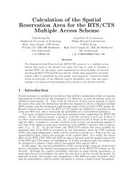
The 17th Annual IEEE International Symposium on Personal, Indoor and Mobile Radio Communications (PIMRC’06)<br />
ANALYSIS OF THE RTS/CTS MULTIPLE ACCESS SCHEME<br />
WITH CAPTURE EFFECT<br />
Chin Keong Ho †§<br />
†Eindhoven University <strong>of</strong> Technology<br />
Eindhoven, The Ne<strong>the</strong>rlands<br />
Jean-Paul M. G. Linnartz §†<br />
§Philips Research Laboratories<br />
Eindhoven, The Ne<strong>the</strong>rlands<br />
ABSTRACT<br />
The Request-to-Send (RTS) / Clear-to-Send (CTS) <strong>scheme</strong><br />
uses a four-way handshake to ensure proper spatial and temporal<br />
reservation <strong>of</strong> <strong>the</strong> <strong>multiple</strong>-<strong>access</strong> wireless LAN channel.<br />
By considering <strong>the</strong> (interdependence <strong>of</strong>) successive <strong>capture</strong><br />
probabilities for a cycle <strong>of</strong> an RTS, CTS, data packet and<br />
acknowledgement, we analyze <strong>the</strong> throughput <strong>of</strong> <strong>the</strong> RTS/CTS<br />
<strong>scheme</strong> in a new ma<strong>the</strong>matical framework. We also propose<br />
closed-form bounds which are useful for rate optimization.<br />
I. INTRODUCTION<br />
The performance <strong>of</strong> today’s wireless LANs is increasingly limited<br />
by mutual interference. Several mechanisms are used to<br />
allow co-existence, such as carrier sensing and virtual sensing.<br />
Carrier sensing is a <strong>multiple</strong> <strong>access</strong> <strong>scheme</strong> that inhibits<br />
transmission when an ongoing transmission is detected at <strong>the</strong><br />
transmitter [1]. However, in some situations users are inhibited<br />
unnecessarily [2]. This could be solved by virtual sensing in<br />
which <strong>the</strong> source first asks <strong>the</strong> destination whe<strong>the</strong>r <strong>the</strong> channel<br />
is idle by a Request-to-Send (RTS) packet, and <strong>the</strong> destination<br />
confirms this <strong>with</strong> a Clear-to-Send (CTS) packet [2]. Remote<br />
stations that recover <strong>the</strong> RTS or CTS packet are inhibited to<br />
transmit during some specified time, hence increasing <strong>the</strong> probability<br />
<strong>of</strong> a successful transmission.<br />
Two types <strong>of</strong> model for packet recovery have been assumed<br />
when considering <strong>the</strong> RTS/CTS <strong>scheme</strong>. In <strong>the</strong> collision<br />
model, a packet is correctly received, i.e., recovered, if and<br />
only if <strong>the</strong>re is no o<strong>the</strong>r concurrent transmission, e.g. [3]. A improved<br />
model is based on <strong>the</strong> power <strong>capture</strong> <strong>effect</strong>: a packet is<br />
recovered (even if <strong>the</strong>re are interfering signals) if and only if <strong>the</strong><br />
signal-to-noise plus interference ratio (SINR) is greater than a<br />
<strong>capture</strong> ratio, e.g. [4, 5]. In <strong>the</strong> literature [3, 4, 5], <strong>the</strong> RTS/CTS<br />
<strong>scheme</strong> has been modeled by assuming that if <strong>the</strong> RTS is recovered<br />
by <strong>the</strong> destination, <strong>the</strong>n <strong>the</strong> CTS, payload (PAY) and<br />
acknowledgement (ACK) will be recovered too. This is in fact<br />
an approximation that violates <strong>the</strong> principle <strong>of</strong> <strong>the</strong> <strong>capture</strong> <strong>effect</strong>.<br />
By removing this approximation, <strong>the</strong> causal <strong>effect</strong> <strong>of</strong> <strong>the</strong><br />
RTS, CTS, PAY and ACK in time is analyzed in [6].<br />
This paper extends <strong>the</strong> results <strong>of</strong> [6] by calculating <strong>the</strong><br />
throughput achieved using <strong>the</strong> RTS/CTS <strong>scheme</strong>. By choosing<br />
appropriate RTS, CTS and PAY transmission rates, we illustrate<br />
by numerical examples how throughput maximization<br />
can be carried out. Moreover, by deriving closed-form throughput<br />
lower bounds, it is shown quantitatively that <strong>the</strong> RTS/CTS<br />
<strong>scheme</strong> is superior to <strong>the</strong> ALOHA <strong>scheme</strong> when <strong>the</strong> PAY length<br />
is sufficiently long (such that that <strong>the</strong> overheads are small) and<br />
when <strong>the</strong> RTS and CTS rates are sufficiently small (such that<br />
<strong>the</strong> interference are low).<br />
<br />
<br />
<br />
<br />
<br />
<br />
<br />
<br />
<br />
<br />
<br />
<br />
<br />
<br />
<br />
<br />
<br />
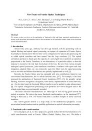
Figure 1: RTS/CTS <strong>multiple</strong> <strong>access</strong> <strong>scheme</strong>.<br />
A. RTS/CTS Scheme<br />
II.<br />
MODEL<br />
<br />
The test station (STA) will be referred to simply as STA and <strong>the</strong><br />
o<strong>the</strong>r STAs as interferers. We assume that STA uses RTS/CTS<br />
for channel <strong>access</strong> to <strong>the</strong> intended destination which we assume<br />
to be <strong>the</strong> <strong>access</strong> point, AP. On <strong>the</strong> o<strong>the</strong>r hand, <strong>the</strong> interferers<br />
use slotted ALOHA for <strong>multiple</strong> <strong>access</strong>.<br />
The detailed RTS/CTS <strong>scheme</strong> considered here is shown in<br />
Fig. 1. A transmission cycle consists <strong>of</strong> an RTS packet, a CTS<br />
packet, a PAY (data) packet and an ACK packet; for conciseness<br />
<strong>the</strong> word “packet” is subsequently omitted when referring<br />
to <strong>the</strong> different packet types. For ease <strong>of</strong> <strong>analysis</strong>, we assume<br />
<strong>the</strong> system to be time slotted. Each RTS, CTS and ACK uses<br />
one slot, and <strong>the</strong> PAY uses P slots. As illustrated, if <strong>the</strong> interferers<br />
recover <strong>the</strong> RTS (CTS), <strong>the</strong>y are inhibited to transmit<br />
during <strong>the</strong> CTS and ACK periods (PAY period, respectivly).<br />
In <strong>effect</strong>, <strong>the</strong> inhibition period is kept to a minimum; this is in<br />
contrast to <strong>the</strong> practice <strong>of</strong> IEEE 802.11, where any inhibition<br />
is carried out continuously until <strong>the</strong> cycle completes. Fur<strong>the</strong>rmore,<br />
we assume:<br />
1) No carrier sensing: In contrast to common practice in<br />
IEEE 802.11, we explicitly do not consider that carrier sensing<br />
is carried out, but only virtual sensing via <strong>the</strong> RTS/CTS mechanism.<br />
This eliminates <strong>the</strong> exposed node problem associated<br />
<strong>with</strong> carrier sensing.<br />
2) Only STA is fully RTS/CTS capable: For analytical<br />
tractability, we assume that only STA uses RTS/CTS for <strong>multiple</strong><br />
<strong>access</strong>. The interferers uses slotted ALOHA. Yet, <strong>the</strong>y<br />
obey <strong>the</strong> RTS/CTS rules, that is, <strong>the</strong>y temporarily refrain from<br />
transmission after <strong>the</strong>y recover any RTS or CTS.<br />
3) Slotted Data Detection: Data is (transmitted and) detected<br />
during PAY on a slot by slot basis, independently <strong>of</strong> o<strong>the</strong>r slots.<br />
As a result, <strong>the</strong> ACK comprises <strong>of</strong> <strong>multiple</strong> acknowledgement<br />
bits, one bit for each slot <strong>of</strong> data. This assumption allows <strong>the</strong><br />
<strong>capture</strong> model to be applied for each slot independently.<br />
1-4244-0330-8/06/$20.00 c○2006 IEEE
The 17th Annual IEEE International Symposium on Personal, Indoor and Mobile Radio Communications (PIMRC’06)<br />
B. Capture, Channel and Network Models<br />
The instantaneous SINR can be represented as<br />
p 0<br />
SINR =<br />
N o + ∑ N<br />
i=1 p , (1)<br />
i<br />
where p 0 , p i is <strong>the</strong> instantaneous signal power <strong>of</strong> STA and <strong>the</strong><br />
i th interferer, respectively, while N o is <strong>the</strong> noise power. From<br />
information <strong>the</strong>ory, when <strong>the</strong> interference and <strong>the</strong> data is independent<br />
Gaussian distributed, an achievable instantaneous<br />
data rate, in bits/symbol, is given by <strong>the</strong> mutual information<br />
I(SINR) = log(1 + SINR). An information outage is said to<br />
occur if <strong>the</strong> instantaneous mutual information is smaller than<br />
R, i.e., when SINR < 2 R − 1.<br />
The <strong>capture</strong> <strong>effect</strong>, channel and network are modeled as follows.<br />
1) Capture Effect: The <strong>capture</strong> <strong>effect</strong> is modeled by assuming<br />
that <strong>the</strong> packet is correctly decoded if and only if <strong>the</strong>re is<br />
no information outage, hence relating <strong>the</strong> <strong>capture</strong> ratio to <strong>the</strong><br />
rate as z(R) 2 R − 1.<br />
2) Path Loss: All transmitters use <strong>the</strong> same power. However,<br />
each signal experiences path loss depending on <strong>the</strong> propagation<br />
distance, a. We model <strong>the</strong> local mean power according to <strong>the</strong><br />
path loss law ¯p = a −β where β = 4 is used in this paper.<br />
3) Channel: Each channel exhibits quasi-static flat Rayleigh<br />
fading during one RTS, CTS, PAY or ACK transmission, but<br />
independent for different transmission links and slots. Hence,<br />
<strong>the</strong> probability density function (pdf) <strong>of</strong> <strong>the</strong> power p is f p (p) =<br />
1<br />
¯p exp (− p¯p<br />
)<br />
.<br />
4) Interferers’ Positions: The x- and y-coordinates <strong>of</strong> <strong>the</strong><br />
STA and AP are denoted by position vectors a STA , a AP , respectively.<br />
When <strong>the</strong> RTS/CTS <strong>scheme</strong> is not implemented,<br />
interfering packets are transmitted according to a homogenous<br />
(spatial) Poisson process <strong>with</strong> intensity G(a) = G o packets per<br />
time slot per unit area, where 0 < G o < ∞ and a is in an operating<br />
region A. The total traffic rate is G t = ∫ G(a) da.<br />
a∈A<br />
In this paper, we let <strong>the</strong> region A grows infinitely large.<br />
III.<br />
CAPTURE PROBABILITY<br />
Consider a source at a source transmitting a packet <strong>of</strong> length L<br />
and rate R to a destination at a dest . The traffic intensity is G(a).<br />
The event that <strong>the</strong> packet is recovered, i.e., that <strong>the</strong> packet <strong>capture</strong>s<br />
<strong>the</strong> receiver, is denoted as E cap (a source , a dest , R, L, G).<br />
The arguments <strong>of</strong> z and E cap will be dropped when <strong>the</strong>re is no<br />
ambiguity.<br />
A. General Capture Probability<br />
Let f pi denote <strong>the</strong> (exponential) pdf <strong>of</strong> <strong>the</strong> power <strong>of</strong> <strong>the</strong> i th<br />
interferer and L f (s) <strong>the</strong> Laplace transform <strong>of</strong> function f evaluated<br />
at s. Define<br />
W (2 R −1, |a source −a dest |, |a i −a dest |) = 1−L fpi ((2 R −1)/¯p).<br />
Then, <strong>the</strong> <strong>capture</strong> probability can be simplified as [7]<br />
{<br />
Pr{E cap } = exp − zN o<br />
¯p<br />
∫a − J (a i ) da i<br />
}, (2)<br />
i∈A<br />
J (a i ) W (z, |a source − a dest |, |a i − a dest |)G(a i ). (3)<br />
B. Data Capture Probability<br />
Let E R , E C , E P and E A respectively denote <strong>the</strong> <strong>capture</strong> events<br />
that a slot <strong>of</strong> <strong>the</strong> RTS, CTS, PAY and ACK are recovered. Note<br />
that for P > 1, E P is <strong>the</strong> <strong>capture</strong> event <strong>of</strong> a given slot during<br />
PAY, but is statistically <strong>the</strong> same for any slot due to <strong>the</strong> assumption<br />
that <strong>the</strong> channel is independent for every slot. The event<br />
that <strong>the</strong> data in a slot carried by <strong>the</strong> PAY is considered to be<br />
transported to <strong>the</strong> destination, denoted as E data , occurs if all<br />
<strong>the</strong> above four <strong>capture</strong> events occurs, since <strong>the</strong> ACK contains<br />
acknowledgement bits for all PAY slots. Hence, <strong>the</strong> probability<br />
that <strong>the</strong> data in a PAY slot is recovered by <strong>the</strong> AP, i.e., <strong>the</strong> data<br />
<strong>capture</strong> probability, can be expressed using <strong>the</strong> chain rule as<br />
Pr(E data ) = Pr(E R , E C , E P , E A )<br />
= Pr(E R ) Pr(E C |E R ) Pr(E P |E R , E C ) Pr(E A |E R , E C , E P ).(4)<br />
Unlike <strong>the</strong> RTS and CTS which inhibits o<strong>the</strong>r users, reducing<br />
<strong>the</strong> ACK rate does not incur any penalty on <strong>the</strong> network. Often,<br />
<strong>the</strong> ACK is transmitted at <strong>the</strong> lowest possible rate to ensure reliable<br />
communication. To make <strong>the</strong> <strong>analysis</strong> concise, we approximate<br />
R A as (<strong>effect</strong>ively) zero and so Pr(E A |E R , E C , E P ) = 1.<br />
Hence, to compute Pr(E data ) <strong>the</strong>n only requires computing <strong>the</strong><br />
first three factors <strong>of</strong> (4).<br />
We use Φ, Θ ∈ {R, C, P, A} to denote a generic packet type.<br />
Fur<strong>the</strong>rmore, E refers to any or some <strong>of</strong> {E R , E C , E P , E A , ∅},<br />
where ∅ denotes a null set. We also use <strong>the</strong> following notations:<br />
1) R Φ is <strong>the</strong> rate used for transmitting Φ;<br />
2) z Φ 2 RΦ − 1 is <strong>the</strong> <strong>capture</strong> ratio;<br />
3) G Φ|E (a) is <strong>the</strong> spatial traffic intensity at a when Φ is transmitted<br />
conditioned on event E; and<br />
4) P Φ|E (a) is <strong>the</strong> probability that Φ <strong>capture</strong>s a receiver at a<br />
conditioned on event E.<br />
Here, <strong>the</strong> position vector a is <strong>the</strong> position <strong>of</strong> an interferer for<br />
<strong>the</strong> traffic intensity or <strong>of</strong> a receiver for <strong>the</strong> <strong>capture</strong> probability.<br />
C. Relationship <strong>of</strong> Traffic Intensity and Capture Probability<br />
Computing any <strong>capture</strong> probability can be carried out using (2)<br />
if <strong>the</strong> traffic intensity is known. Hence, <strong>the</strong> problem <strong>of</strong> finding<br />
<strong>the</strong> <strong>capture</strong> probability is reduced to finding <strong>the</strong> corresponding<br />
traffic intensity. Based on <strong>the</strong> RTS/CTS <strong>scheme</strong> described in<br />
Sect. A., <strong>the</strong> <strong>capture</strong> probability for different packet types at a<br />
is<br />
P R|E (a) = Pr { E cap (a STA , a, R R , G R|E ) } , (5)<br />
P C|E (a) = Pr { E cap ( a AP , a, R C , G C|E ) } , (6)<br />
P P|E (a) = Pr { E cap (a STA , a, R P , G P|E ) } . (7)<br />
The individual <strong>capture</strong> probability <strong>of</strong> (4) can <strong>the</strong>n be expressed<br />
concisely as special cases <strong>of</strong> (5), (6), (7), respectively:<br />
Pr(E R ) = P R (a AP ), (8)<br />
Pr(E C |E R ) = P C|ER (a STA ), (9)<br />
Pr(E P |E R , E C ) = P P|ER,E C<br />
(a AP ). (10)<br />
D. Capture Probabilities Pr(E R ), Pr(E C |E R ), Pr(E P |E R , E C )<br />
We summarized <strong>the</strong> computations required to calculate<br />
Pr(E R ), Pr(E C |E R ), Pr(E P |E R , E C ); details are provided in
The 17th Annual IEEE International Symposium on Personal, Indoor and Mobile Radio Communications (PIMRC’06)<br />
(12)<br />
↦→ G R|ER (a) (5)<br />
−→ P R|ER (a) (13)<br />
−→ G C|ER (a) (6)<br />
−→ P C|ER (a) (9)<br />
−→ Pr(E C |E R )<br />
Figure 2: Relationship <strong>of</strong> <strong>capture</strong> probabilities and traffic intensities over time and space in calculating Pr(E C |E R ).<br />
· · · → G C|ER (a) (14)<br />
−→ G C|ER,E C<br />
(a) (6)<br />
−→ P C|ER,E C<br />
(a) (15)<br />
−→ G P|ER,E C<br />
(a) (7)<br />
−→ P P|ER,E C<br />
(a) (10)<br />
−→ Pr(E P |E R , E C )<br />
Figure 3: Relationship <strong>of</strong> <strong>capture</strong> probabilities and traffic intensities over time and space in calculating Pr(E P |E R , E C ).<br />
[6]. To emphasis <strong>the</strong> effe<strong>cts</strong> <strong>of</strong> interference, we consider <strong>the</strong><br />
case when <strong>the</strong> noise is negligible, i.e., N o = 0.<br />
The RTS <strong>capture</strong> probability can be derived in closed-form<br />
as<br />
Pr(E R ) = exp { −a 2 sπ 2 G o<br />
√<br />
zR /2 } (11)<br />
where a s = |a STA − a AP | is <strong>the</strong> distance between STA and AP.<br />
On <strong>the</strong> o<strong>the</strong>r hand, <strong>the</strong> conditional CTS <strong>capture</strong> probability is<br />
fairly difficult to compute, given by <strong>the</strong> sequence <strong>of</strong> computation<br />
(as time progresses in <strong>the</strong> RTS/CTS cycle) in Fig. 2. To<br />
complete <strong>the</strong> computation, <strong>the</strong> conditional traffic intensities can<br />
be shown to be<br />
G R|ER (a) = G o (1 − W (z R , a s , |a − a AP |)), (12)<br />
G C|ER (a) = G o<br />
(<br />
1 − PR|ER (a) ) . (13)<br />
Similarly, <strong>the</strong> conditional PAY <strong>capture</strong> probability is computed<br />
as shown in Fig. 3 using <strong>the</strong> following conditional traffic<br />
intensities<br />
G C|ER,E C<br />
(a) = (1 − W (z C , a s , |a − a STA |))G C|ER (a),(14)<br />
G P|ER,E C<br />
(a) = G o<br />
(<br />
1 − PC|ER,E<br />
C<br />
(a)) ) . (15)<br />
Note that G C|ER is required to start <strong>the</strong> computation and is available<br />
from Fig. 2.<br />
IV.<br />
LOWER BOUND CAPTURE PROBABILITIES<br />
Closed-form expressions ease optimization studies, specifically<br />
for throughput maximization. Although Pr(E R ) is available<br />
in closed form, exact closed forms for <strong>the</strong> conditional CTS<br />
and PAY <strong>capture</strong> probabilities are not available. Instead, lower<br />
bound closed forms are derived here.<br />
A general approach to lower bound <strong>the</strong> <strong>capture</strong> probability<br />
during Φ is to upper bound <strong>the</strong> corresponding traffic intensity<br />
during Φ. We show that this upper bound traffic intensity can be<br />
obtained by using a uniform upper bound traffic intensity during<br />
Θ where Θ occurs before Φ. By choosing Θ appropriately,<br />
a closed-form for <strong>the</strong> <strong>capture</strong> probability can <strong>the</strong>n be obtained.<br />
All lower bound <strong>capture</strong> probabilities are denoted by capping<br />
<strong>the</strong> exact ones <strong>with</strong> tildes; all upper bound traffic intensities are<br />
denoted similarly.<br />
A. Lower Bound CTS Capture Probability<br />
We proceed in <strong>the</strong> forward time sense as indicated by <strong>the</strong> arrows<br />
in Fig. 2. From (12), a valid upper bound <strong>of</strong> G R|ER (a) is<br />
G o since it can be shown that <strong>the</strong> W function is always positive.<br />
This gives us a lower bound to P R|ER (a), which can be<br />
appreciated by observing <strong>the</strong> relationship <strong>of</strong> <strong>the</strong> <strong>capture</strong> probability<br />
and <strong>the</strong> traffic intensity in (2). Since <strong>the</strong> upper bound<br />
traffic is uniform, <strong>the</strong> lower bound <strong>capture</strong> probability is <strong>the</strong><br />
same as <strong>the</strong> RTS <strong>capture</strong> probability, <strong>the</strong>refore<br />
˜P R|ER (a) = exp { −b 2 π 2 G o<br />
√<br />
zR /2 } (16)<br />
where b = |a STA − a|. From (16) and (13), we <strong>the</strong>n obtain an<br />
upper bound to G C|ER (a) as<br />
˜G C|ER (a) = G o<br />
(1 − ˜P<br />
)<br />
R|ER (a)<br />
(17)<br />
which can be alternatively written as function <strong>of</strong> b, i.e., as<br />
˜G C|ER (b). Using (2) <strong>with</strong> transformation <strong>of</strong> <strong>the</strong> random variable<br />
from a to b, <strong>the</strong> desired lower bound is<br />
{ ∫ ∞<br />
}<br />
˜Pr(E C |E R ) = exp − 2πbW (z C , a s , b) ˜G C|ER (b) db , (18)<br />
0<br />
where noise is assumed to be absent. After some derivations<br />
(omitted due to lack <strong>of</strong> space), we obtain<br />
˜Pr(E C |E R ) = exp{a 2 sπG o<br />
√<br />
zC × g(G o π 2 a 2 s√<br />
zC z R /2)<br />
−a 2 sπ 2 G o<br />
√<br />
zC /2} (19)<br />
where g(s) cos(s) [ π<br />
2 − Si(s)] + sin(s)Ci(s), Si(s) =<br />
∫ π 2 −<br />
∞ sin y<br />
s y<br />
dy is <strong>the</strong> sine integral and Ci(s) = − ∫ ∞ cos y<br />
s y<br />
dy <strong>the</strong><br />
cosine integral.<br />
B. Lower Bound PAY Capture Probability<br />
The lower bound for PAY follows <strong>the</strong> same derivation as that<br />
for CTS. We proceed according to Fig. 3. First we bound<br />
G C|ER,E C<br />
(a) by G o . This is valid as seen from (14) and (13).<br />
Carrying on <strong>the</strong> arguments in a similar way, we arrive at<br />
˜P C|ER,E C<br />
(a) = exp { −b 2 π 2 √<br />
G o zC /2 } , (20)<br />
˜G P|ER,E C<br />
(a) = G o<br />
(1 − ˜P<br />
)<br />
C|ER,E C<br />
(a) , (21)<br />
where b = |a AP − a|. Therefore, similar to <strong>the</strong> derivation <strong>of</strong><br />
(19), <strong>the</strong> <strong>capture</strong> probability for <strong>the</strong> PAY is lower bounded by<br />
˜Pr(E P |E R , E C ) = exp{a 2 sπG o<br />
√<br />
zP · g(G o π 2 a 2 s√<br />
zP z C /2)<br />
A. Analysis<br />
−a 2 sπ 2 G o<br />
√<br />
zP /2}. (22)<br />
V. THROUGHPUT<br />
For <strong>the</strong> purpose <strong>of</strong> <strong>analysis</strong>, we assume that <strong>the</strong> RTS/CTS cycles<br />
are spaced sufficiently far apart so that <strong>the</strong> inhibition period<br />
<strong>of</strong> one cycle do not overlap <strong>with</strong> <strong>the</strong> next . We consider<br />
<strong>the</strong> throughput <strong>of</strong> <strong>the</strong> RTS/CTS <strong>scheme</strong> averaged over <strong>the</strong> time<br />
when STA <strong>access</strong>es <strong>the</strong> channel via RTS/CTS.
The 17th Annual IEEE International Symposium on Personal, Indoor and Mobile Radio Communications (PIMRC’06)<br />
The last line <strong>of</strong> (27) is obtained by using (4) and assuming<br />
Consider <strong>the</strong> possible cases when a cycle is terminated from<br />
where Ω(P ) <br />
P Pr(E R , E C )<br />
2 + (P + 1) Pr(E R , E C ) . (28) ing <strong>the</strong> slotted ALOHA is plotted in Fig. 4. We assumed for<br />
simplicity that ACK is not required for ALOHA and hence<br />
<strong>the</strong> STA’s perspective. There are only two, ei<strong>the</strong>r when (i) STA Pr(E A |E R , E C , E P ) = 1.<br />
does not recover <strong>the</strong> CTS (including <strong>the</strong> case that <strong>the</strong> CTS may<br />
not be sent by <strong>the</strong> AP in <strong>the</strong> first place because <strong>the</strong> RTS is not<br />
recovered), or when (ii) STA has received <strong>the</strong> ACK (but may<br />
not necessarily recover it). These cases are indicated respectively<br />
Property 1 For a given R R , R C , R P , <strong>the</strong> throughput ¯s is an<br />
increasing function <strong>of</strong> P . Hence, an upper bound is given by<br />
<strong>the</strong> asymptotic throughput<br />
as {R, C}, {R, C, P, A}. The first case occurs if <strong>the</strong> RTS<br />
or <strong>the</strong> CTS is not recovered <strong>with</strong> probability<br />
lim P Pr(E P |E R , E C ).<br />
P →∞<br />
(29)<br />
Pr(ĒR) + Pr(E R , ĒC) = 1 − Pr(E R , E C ), (23)<br />
Pro<strong>of</strong> 1 Note that R P Pr(E P |E R , E C ) in (27) is independent<br />
where Ē indicates <strong>the</strong> complement <strong>of</strong> event E. The second case,<br />
<strong>the</strong>refore, occurs <strong>with</strong> probability Pr(E R , E C ).<br />
The duration <strong>of</strong> each cycle <strong>of</strong> <strong>the</strong> RTS/CTS transmission,<br />
<strong>of</strong> P , while as P increases, Ω(P ) increases (hence proving<br />
<strong>the</strong> first statement <strong>of</strong> <strong>the</strong> proposition) and approaches 1 (hence<br />
proving <strong>the</strong> second).<br />
i.e., <strong>the</strong> cycle time, is i.i.d. As a result, <strong>the</strong> cycle time is a<br />
renewal process. Let s t ∈ {0, L sym × R P } be <strong>the</strong> amount <strong>of</strong><br />
bits recovered in slot t, where L sym is <strong>the</strong> number <strong>of</strong> symbols<br />
Property 2 For any given R R , R C , P , <strong>the</strong> optimal R P that<br />
maximizes ¯s is <strong>the</strong> same.<br />
sent per slot. Note that s t can be greater than zero only during<br />
PAY period, o<strong>the</strong>rwise it is zero since only overheads are sent. Pro<strong>of</strong> 2 When R R , R C , P are given, Ω(P ) is independent <strong>of</strong><br />
By using <strong>the</strong> renewal-reward <strong>the</strong>orem [8], <strong>the</strong> time average <strong>of</strong> R P while R P and Pr(E P |E R , E C ) are functions <strong>of</strong> R P . Hence,<br />
<strong>the</strong> throughput in bit/symbol over an infinitely large period is maximizing ¯s is equivalent to maximizing (29), and is independent<br />
<strong>of</strong> <strong>the</strong> actual values <strong>of</strong> R R , R C , P .<br />
1 1<br />
N∑<br />
¯s(a s , R R , R C , R P , P ) lim<br />
s t<br />
N→∞ L sym N<br />
From Properties 1, 2, it follows that for any given R R , R C , <strong>the</strong><br />
t=1<br />
maximum throughput ¯s obtained by optimizing R P increases<br />
1 E [R]<br />
=<br />
(24) <strong>with</strong> P . This is because increasing P reduces <strong>the</strong> overhead and<br />
L sym E [T ]<br />
does not have any negative effe<strong>cts</strong>, which follows intuitively<br />
<strong>with</strong> probability 1. Here, <strong>the</strong> expectation E is carried out over<br />
<strong>the</strong> events in one cycle, R is <strong>the</strong> reward in <strong>the</strong> form <strong>of</strong> <strong>the</strong> sum<br />
<strong>of</strong> s t in a cycle, and T is <strong>the</strong> cycle time in slots. As explicitly<br />
denoted, <strong>the</strong> time averaged throughput is a function <strong>of</strong> many<br />
parameters. We take a s to be fixed, and consider how <strong>the</strong> rates<br />
and PAY length P affect <strong>the</strong> throughput. For notational convenience,<br />
<strong>the</strong> arguments <strong>of</strong> ¯s are dropped.<br />
On average, P Pr(E data ) slots are successful during <strong>the</strong> PAY<br />
period. Hence, <strong>the</strong> expected reward is<br />
from <strong>the</strong> fact that <strong>the</strong> data are detected independently on a slot<br />
by slot basis.<br />
To improve <strong>the</strong> reliability <strong>of</strong> <strong>the</strong> data, <strong>the</strong> lowest practical<br />
rate for R R , R C may be chosen to ensure <strong>the</strong> largest reservation<br />
<strong>effect</strong> over space. However, it may be necessary to reduce <strong>the</strong><br />
amount <strong>of</strong> inhibition, in which case moderate values <strong>of</strong> rates<br />
may be chosen. After R R , R C are fixed, as a consequence <strong>of</strong><br />
Properties 1, 2, we can choose P as large as practically possible<br />
and also independently optimize R P for <strong>the</strong> given R R , R C .<br />
E [R] = L sym R P P Pr(E data ) (25) Property 3 A lower bound <strong>of</strong> ¯s is obtained by substituting <strong>the</strong><br />
Taking into account that <strong>the</strong> cases {R, C}, {R, C, P, A} use 2 <strong>capture</strong> probabilities in (27) <strong>with</strong> <strong>the</strong>ir lower bounds (19), (22).<br />
and P + 3 slots, respectively, <strong>the</strong> expected cycle time is<br />
P<br />
Pro<strong>of</strong> 3 By rewriting Ω(P ) =<br />
2/ Pr(E R,E C)+(P +1)<br />
, we obtain<br />
E [T ] = 2(1 − Pr(E R , E C )) + (P + 3) Pr(E R , E C )<br />
= 2 + (P + 1) Pr(E R , E C ). (26)<br />
P<br />
¯s ≥ ˜s R P˜Pr(EP |E R , E C )<br />
This result can be explained as follows. From (26), it is seen<br />
2/˜Pr(E R , E C ) + (P + 1) . (30)<br />
that at least two slots are used for <strong>the</strong> cycle. This overhead corresponds<br />
to <strong>the</strong> RTS and CTS slot since STA has to wait for <strong>the</strong><br />
B. Numerical Results<br />
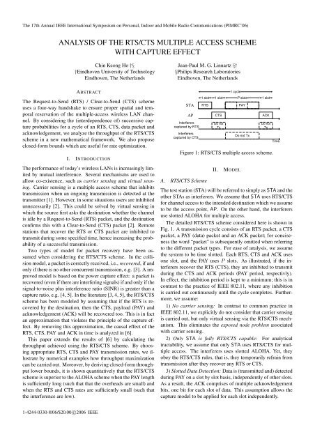
CTS to arrive before deciding to transmit PAY or to defer <strong>the</strong> The throughput ¯s vs R P is plotted in Fig. 4. The following system<br />
parameters are fixed: R R = R C = 0.5, a s = 0.5, G o =<br />
transmission. Subsequently, if <strong>the</strong> RTS and CTS are recovered<br />
(<strong>with</strong> probability Pr(E R , E C )), P slots are used for PAY and 1/π, while P are varied. For a fixed P , as R P increases,<br />
one slot for a potential ACK. The potential ACK requires one ¯s increases initially, peaking at some R P , say RP o (P ), <strong>the</strong>n<br />
slot since STA has to spend time receiving <strong>the</strong> ACK regardless decreases. This is because transmitting at a low R P limits<br />
<strong>of</strong> whe<strong>the</strong>r it is actually sent by <strong>the</strong> AP.<br />
<strong>the</strong> throughput, while transmitting at a high R P reduces <strong>the</strong><br />
Using (25) and (26), (24) becomes<br />
throughput as <strong>the</strong> PAY becomes unreliable. Fur<strong>the</strong>rmore, as P<br />
increases, <strong>the</strong> throughput increases for any fixed R P , as stated<br />
R P P Pr(E data )<br />
¯s =<br />
in Property 1. From Fig. 4, Property 2 is also apparent, since<br />
2 + (P + 1) Pr(E R , E C )<br />
<strong>the</strong> RP o (P ) = 3.6 for all P .<br />
= R P Pr(E P |E R , E C ) × Ω(P ), (27) In addition, <strong>the</strong> throughput when STA transmits to AP us-
The 17th Annual IEEE International Symposium on Personal, Indoor and Mobile Radio Communications (PIMRC’06)<br />
2.5<br />
2<br />
RTS/CTS, P=1<br />
RTS/CTS, P=2<br />
RTS/CTS, P=10<br />
RTS/CTS, P=50<br />
RTS/CTS, P→ ∞<br />
RTS/CTS, lower bound, P→ ∞<br />
2.5<br />
2<br />
RTS/CTS, lower bound, P=1<br />
RTS/CTS, lower bound, P=2<br />
RTS/CTS, lower bound, P=5<br />
RTS/CTS, lower bound, P=10<br />
RTS/CTS, lower bound, P=50<br />
RTS/CTS, lower bound, P→ ∞<br />
throughput (bit/symbol)<br />
1.5<br />
1<br />
ALOHA<br />
throughput (bit/symbol)<br />
1.5<br />
1<br />
Maximum ALOHA throughput<br />
0.5<br />
0.5<br />
3.1<br />
3.6<br />
0<br />
0 1 2 3 4 5 6<br />
Rate <strong>of</strong> PAY, R P<br />
, or rate <strong>of</strong> ALOHA, R ALOHA<br />
0<br />
0 0.5 1 1.5 2 2.5 3 3.5 4 4.5 5<br />
R R<br />
( = R C<br />
)<br />
Figure 4: Throughput ¯s vs rate <strong>of</strong> PAY slots R P for various<br />
packet length P . The analytical lower bound when P → ∞,<br />
and <strong>the</strong> throughput for ALOHA transmission are also plotted.<br />
The stars indicates where <strong>the</strong> maximum throughput is achieved.<br />
Parameters: R R = R C = 0.5, a s = 0.5, G o = 1/π.<br />
no overhead is incurred. The ALOHA throughput is <strong>the</strong>n<br />
given by <strong>the</strong> data rate, say R ALOHA , multiplied by <strong>the</strong> (noninhibiting)<br />
<strong>capture</strong> probability, i.e., (11) <strong>with</strong> z R replaced by<br />
z ALOHA = 2 RALOHA − 1. It is seen that <strong>the</strong> maximum throughput<br />
<strong>of</strong> <strong>the</strong> RTS/CTS <strong>scheme</strong> can be significantly larger than<br />
that <strong>of</strong> <strong>the</strong> ALOHA <strong>scheme</strong>. For example, when P = 50<br />
and R P ≥ 0.1, <strong>the</strong> RTS/CTS <strong>scheme</strong> is always better than <strong>the</strong><br />
ALOHA <strong>scheme</strong> for R P = R ALOHA .<br />
Consider <strong>the</strong> throughput lower bound ˜s when P → ∞, also<br />
plotted in Fig. 4. It is possible to approximate RP o from <strong>the</strong><br />
lower bound, hence giving a simple method for performing rate<br />
adaption for <strong>the</strong> PAY slots. Moreover, using <strong>the</strong> optimal rate<br />
obtained from <strong>the</strong> lower bound at R P = 3.1, a throughput that<br />
is fairly close to <strong>the</strong> maximum possible is achieved. For example,<br />
for P → ∞, a throughput <strong>of</strong> 2.085 bit/symbol is achieved<br />
at R P = 3.1. There is a slight loss <strong>of</strong> 0.041 bit/symbol compared<br />
to <strong>the</strong> optimal throughput <strong>of</strong> 2.126 bit/symbol achieved<br />
at RP o = 3.6.<br />
Lastly, we obtain a conservative estimate <strong>of</strong> <strong>the</strong> maximum<br />
RTS/CTS throughput by maximizing R P over <strong>the</strong> analytical<br />
lower bound ˜s. For simplicity, we set R R = R C although fur<strong>the</strong>r<br />
optimization <strong>of</strong> <strong>the</strong> two rates could yield larger throughput.<br />
From Fig. 5, increasing R R = R C reduces <strong>the</strong> RTS/CTS<br />
throughput since <strong>the</strong> amount <strong>of</strong> interference increases correspondingly,<br />
while increasing P increases <strong>the</strong> throughput since<br />
<strong>the</strong> overhead used becomes negligible. The ALOHA throughput,<br />
optimized over R ALOHA , is also plotted. The ALOHA<br />
throughput is a constant since it does not change <strong>with</strong> R R or<br />
R C . It is observed that <strong>the</strong> lower bound RTS/CTS throughput<br />
is larger than <strong>the</strong> ALOHA throughput <strong>of</strong> 1.1 when R R is sufficiently<br />
small (to ensure adequate reservation) and P is sufficiently<br />
large (to compensate for <strong>the</strong> overhead).<br />
Figure 5: Lower bound RTS/CTS throughput maximized over<br />
R P , plotted against R R = R C . For sufficiently small R R and<br />
sufficiently large P , <strong>the</strong> RTS/CTS throughput is larger than <strong>the</strong><br />
ALOHA throughput. Parameters: a s = 0.5, G o = 1/π.<br />
VI.<br />
CONCLUSION<br />
It is shown how <strong>the</strong> <strong>capture</strong> probabilities can be used to perform<br />
throughput optimization via rate adaptation and <strong>the</strong> RTS/CTS<br />
<strong>scheme</strong> attains higher throughput than ALOHA when <strong>the</strong> RTS<br />
and CTS rates are sufficiently small and when <strong>the</strong> payload<br />
packet is sufficiently large. Due to <strong>the</strong> large degree <strong>of</strong> freedom<br />
<strong>of</strong>fered by rate adaptations, o<strong>the</strong>r system level optimizations<br />
can also be conducted, such as to improve o<strong>the</strong>r quality<br />
<strong>of</strong> service.<br />
REFERENCES<br />
[1] L. Kleinrock and F. Tobagi, “Packet switching in radio channels: Part I–<br />
carrier sense <strong>multiple</strong>-<strong>access</strong> modes and <strong>the</strong>ir throughput-delay characteristics,”<br />
IEEE Trans. Commun., vol. 23, no. 12, pp. 1400–1416, Dec. 1975.<br />
[2] P. Karn, “MACA- a new channel <strong>access</strong> method for packet radio,” in<br />
ARRL/CRRL Amateur Radio 9th Computer Networking Conference, Sept.<br />
1990, pp. 134–140.<br />
[3] G. Bianchi, “IEEE 802.11-saturation throughput <strong>analysis</strong>,” IEEE Commun.<br />
Lett., vol. 2, no. 12, pp. 318–320, Dec. 1998.<br />
[4] Z. Hadzi-Velkov and B. Spasenovski, “Capture <strong>effect</strong> in IEEE 802.11 basic<br />
service area under influence <strong>of</strong> Rayleigh fading and near/far <strong>effect</strong>,”<br />
in Proc. 13th IEEE Personal, Indoor and Mobile Radio Communications,<br />
vol. 1, Lisbon, Portugal, Sept. 2002, pp. 172–176.<br />
[5] J. H. Kim and J. K. Lee, “Capture effe<strong>cts</strong> <strong>of</strong> wireless CSMA/CA protocols<br />
in Rayleigh and shadow fading channels,” IEEE Trans. Veh. Technol.,<br />
vol. 48, no. 4, pp. 1277–1286, July 1999.<br />
[6] C. K. Ho and J. P. M. G. Linnartz, “Calculation <strong>of</strong> <strong>the</strong> spatial reservation<br />
area for <strong>the</strong> <strong>rts</strong>/<strong>cts</strong> <strong>multiple</strong> <strong>access</strong> <strong>scheme</strong>,” in WIC Twenty-seventh Symposium<br />
on Information Theory in <strong>the</strong> Benelux, Noordwijk, The Ne<strong>the</strong>rlands,<br />
June 2006, pp. 181–188.<br />
[7] J. P. M. G. Linnartz, “Slotted ALOHA land-mobile radio networks <strong>with</strong><br />
site diversity,” IEE Proc.-I, vol. 139, no. 1, pp. 58–70, Feb. 1992.<br />
[8] R. G. Gallager, Discrete Stochastic Processes. Boston: Kluwer Academic<br />
Publishers, 1996.