The Direct Wave Form Digital Filter Structure - Signal Processing ...

The Direct Wave Form Digital Filter Structure:
an Easy Alternative for the Direct Form
Jean H.F. Ritzerfeld
Technische Universiteit Eindhoven, Fac. Elektrotechniek
P.O. Box 513, 5600 MB Eindhoven, The Netherlands
Phone: +31 (0)40 247 3252 Fax: +31 (0)40 246 6508
E-mail: j.h.f.ritzerfeld@tue.nl
Abstract— Although the Direct Form is still widely used
in IIR digital filter design, this structure is known to have
a high coefficient sensitivity and to produce high levels of
quantization noise. Even if only second-order sections are
used to design higher order filters, the sections with poles
close to the unit circle and/or with angles close to 0 or π have
unacceptably high noise levels, specifically in fixed-point applications.
As an easy alternative for the second-order Direct
Form we present the second-order Direct Wave Form. Comparable
to the Direct Form, this structure uses only five multipliers
which are directly linked to the five coefficients of
a general second-order transfer function. It is shown how
the Direct Wave From can be properly scaled with an L 2
scaling measure as well as with the more conservative L ∞
scaling measure. It is then shown, by looking at the secondorder
modes of a general second-order transfer function that
the Direct Wave Form has a superior noise behaviour that is
close to being optimal (within 3dB). The Direct Wave Form
is also shown to be overflow stable and free from limit cycles.
Keywords—Digital filter design; wave digital filters; quantization
noise; scaling, second-order modes.
I. INTRODUCTION
When designing higher order IIR filters, it is common
practice to implement them as a cascade or parallel connection
of second-order sections with transfer functions of
the general form
H(z) = dz2 + ez + f
z 2 − az − b , (1)
having five degrees of freedom. These sections are then
implemented as second-order Direct Forms where the five
degrees of freedom appear as multipliers in the signal flow
graph. For those sections, however, that have poles close
to the unit circle and/or with angles close to 0 or π, the
coefficient sensitivity and the quantization noise become
unacceptably high, specifically in fixed-point applications.
Alternative solutions are then looked for [1], such as the
Normal Form and the Optimal (i.e. minimum-noise) Form,
both of which use extra degrees of freedom to achieve a
better sensitivity/noise behaviour at the cost of extra multipliers
and a less straightforward design, since the one-onone
relation between the values of the multipliers and the
coefficients of the transfer function is lost.
In Section II the Direct Wave Form (DWF) is presented
as an easy alternative for the Direct Form that is as straightforward
to design and uses no extra multipliers. The DWF
has a superior coefficient sensitivity and a noise behaviour
that is close to that of the Optimal Form. In order to scale
the structure to prevent overflow, two scaling multipliers
are introduced, the values of which are given in closed
form using an L 2 (Section II) and an L ∞ scaling measure
(Section IV). These extra multipliers can be given powerof-two
values (to be implemented as shift operations), so
the number of multipliers need not increase. As a quality
measure for the noise behaviour the noise gain of the L 2 -
scaled structure is used, i.e. the scaled power gain of the
quantization noise at is its source (q 2 /12) to the output.
In Section III a simple proof that uses the second-order
modes of the general H(z) is given to show that the DWF
has a noise gain that cannot exceed the minimum noise
gain of the Optimal Form by more than a factor two.
II. THE DIRECT WAVE FORM
In order to arrive at the Direct Wave Form, we start with
Direct Form II (DF2) that has a state-space description
s[n + 1] = As[n] + Bx[n],
y[n] = Cs[n] + Dx[n],
where s = ((s 1 , s 2 )
t is the state ( vector ) and the four matrices
a b
1
are A = , B = , C = (e + ad, f + bd),
1 0
0
D = (d), to realize the transfer function given by (1).
For use in our noise calculations, we also look at the
controllability matrix K = ∑ ∞
k=0 (A k B)(A k B) t and the
observability matrix W = ∑ ∞
k=0 (CA k ) t (CA k ). On the
principal diagonals of these matrices are the power gains
from input to state and from state to output, respectively
(and the cross-power gains on the off-diagonals) [2]. The
scaled noise gain, to be used as a quality measure, is then
G = K 11 W 11 + K 22 W 22 . (2)

For DF2, K and W can be given in closed form [1]:
( )
1 − b a
a 1 − b
K =
(3)
(1 + b)(1 − a − b)(1 + a − b)
and W has entries
W 11 = (1 − b)(c2 1 + c2 2 ) + 2ac 1c 2
(1 + b){(1 − b) 2 − a 2 } , W 22 = b 2 W 11 + c 2 2
W 12 = W 21 = ab(c2 1 + c2 2 ) + (1 − a2 − b 2 )c 1 c 2
(1 + b)(1 − a − b)(1 + a − b) , (4)
where c 1 and c 2 are the elements of C = (e+ad, f +bd).
Note, incidentally, that W 11 is just equal to the quadratic
form CKC t , and that W 22 can also be written as W 11 −
{(1 − b)c 1 + ac 2 } 2 /{(1 − b) 2 − a 2 }, so W 22 ≤ W 11 .
The Direct Wave Form arises from a state transformation
(a rotation in the state plane) applied to DF2. It has a
recursive part that is remindful of a wave digital filter [3],
hence the designation. The state description follows from
the matrices A , B , C , D of DF2 via a similarity transformation
A w = T −1 AT , B w = ( T −1 B, C)
w = CT and
D w = D, where T is taken as 1 1 −1
2
. We find:
1 1
A w =
( ) (
1 − γ1 −γ 2
1
, B
γ 1 −1 + γ w =
2 −1
C w = (η 1 − γ 1 d, η 2 − γ 2 d) and D w = (d), (5)
where γ 1 = 1 2 (1 − a − b), γ 2 = 1 2
(1 + a − b), and where
η 1 = 1 2 (d + e + f), η 2 = 1 2
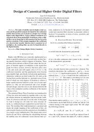
(d − e + f). Fig. 1 depicts
the Direct Wave Form, which is as yet unscaled and uses
only five multipliers directly related to the five coefficients
of H(z), as does the Direct Form. Incidentally, apart from
a factor 1 2
, the γ’s are simply found from evaluating the
denominator of H(z) at z = ±1, whereas the η’s are found
from the numerator at z = ±1.
In order to L 2 -scale the DWF, we need to calculate its
controllability matrix, which proves to be diagonal:
( )
4γ2 0
0 4γ
K w = T −1 KT −t 1
=
4γ 1 γ 2 (2 − γ 1 − γ 2 ) , (6)
where the denominator is the same as that of K in (3), as
governed by the stability triangle of a Direct Form in the
(a, b)-plane: 1+b > 0, 1−a−b > 0, 1+a−b > 0. For the
DWF, the region of linear stability is also a triangle in the
(γ 1 , γ 2 )-plane given by: γ 1 > 0, γ 2 > 0, 2−γ 1 −γ 2 > 0.
In Fig. 2 the L 2 -scaled DWF is drawn, where two extra
multipliers 1/ √ K w11 and 1/ √ K w 22 are introduced.
)
,
✲
✻
z −1 ✛ ❄
s 1 [n] ✛
♥+
❄
❆ ✁
❄
✻ η 1 ❆
✁
❆ ✁
❆✁
❆ ✁ −γ 1
❆✁
x[n] ❄
✲ ♥+
✲ ❍ ❍
❄y[n]
✲ d ❍✟ ✲ ♥+ ✲
✻
✟ ✻
✁❆
✁
✁
❆ −γ 2
❆
✻
z −1 ✛ ✟✟✟ ❍ ✛ + ♥ ❄ η 2
✁ ✁✁❆ ❆
s 2 [n] ✛ −1
❆
❍
✻
❄
✻
✲
✲
Fig. 1. Unscaled Direct Wave Form, where the multipliers are
given by γ 1 = 1 2 (1−a−b), γ 2 = 1 2 (1+a−b), η 1 = 1 2 (d+e+f),
η 2 = 1 2
(d − e + f), realizing the general transfer function (1).
In essence, the scaled DWF of Fig. 2 is the same as the
Wave Digital Form derived in [1]. The difference is that in
the DWF the non-state node x[n] − γ 1 s 1 [n] − γ 2 s 2 [n] is
used explicitly to create the output y[n] via the coefficient
d, much in the same way as the non-state node s 1 [n + 1]
in DF2 is connected to the multiplier d to compute y[n]. In
this sense, the DWF is much more analogous to the Direct
Form, hence the designation. Also, the η’s in Figs. 1 and 2
are more directly related to the coefficients of H(z) than
the elements of C w , which would appear as multipliers if
y[n] were computed in the normal ‘state-space’ way with
d directly connecting x[n] and y[n].
✲
✻
z −1 ✛ ❄
s 1 [n] ✛
♥+
❄
√ ❆ ✁
❄
✻ η 1 k11 ❆
✁
❆ ✁ √ ❆✁
❆ ✁ −γ
❆✁
1 k11
✁ ✁✁❆ ❆1/ √ k 11 ❆
x[n] ❄
✻
✲ ♥+
✲ ❍ ❍
❄y[n]
✲ d ❍✟ ✲ ♥+ ✲
✻
✟ ❄
✻
✁❆
√
✁
✁
❆
❆ ✁
−γ 2 k22 ❆
✁ 1/ √ k 22
❆
❆✁
√
✻
z −1 ✛ ✟✟✟ ❍ ✛ + ♥ ❄ η 2 k22
✁ ✁✁❆ ❆
s 2 [n] ✛ −1
❆
❍
✻
❄
✻
✲
✲
Fig. 2. L 2 -scaled Direct Wave Form, where the extra scaling
multipliers are given by 1/ √ K 11 = √ γ 1 (2 − γ 1 − γ 2 ) and
1/ √ K 22 = √ γ 2 (2 − γ 1 − γ 2 ), as determined by K w in (6).
✲
✲

And finally, more so than the Wave Digital Form in [1],
the DWF is a universal ‘biquad’, i.e. an IIR second-order
section to create the standard filter types in a generic way.
For example, taking η 1 = η 2 = 0 creates a bandpass filter
(zeros at ±1), while high- and lowpass filters result from
either η 1 = 0, or η 2 = 0. Next, if we take d = − 1 2
(1+b) in
the bandpass solution and add x[n] to the output, a bandstop
filter is created with transfer function
− 1 2 (1+b) z 2 1
− 1
z 2 − az − b +1 = 2 (1 − b)z2 −az + 1 2
(1 − b)
z 2 ,
− az − b
(7)
which has unity gain at the frequency edges ϑ = 0 and ϑ =
π and a stop frequency ϑ = arccos{a/(1 − b)}. Likewise,
taking d = −(1 + b) and adding x[n] to the output results
in a unity gain allpass filter:
z 2 − 1
−(1 + b)
z 2 − az − b + 1 = −bz2 − az + 1
z 2 − az − b . (8)
So, the filter types bandpass, bandstop and allpass use only
three multipliers in the unscaled structure and five in the
scaled version (since η 1 = η 2 = 0).
III. NOISE GAIN AND SECOND-ORDER MODES
The noise gain G w = K w11 W w11 + K w 22 W w 22 of the
DWF can be shown to be near-optimal without actually
calculating it. Due to the fact that K w is diagonal, we
can also write G w = tr(K w W w ), where tr(·) denotes the
trace of a matrix, i.e. the sum of the elements on its principal
diagonal. Since under a state transformation with any
(regular) matrix T the product matrix KW is subject to
a similarity transformation T −1 (KW )T , its eigenvalues
(denoted µ 2 1 and µ2 2 ), trace and determinant are invariant.
The square roots µ 1 and µ 2 of these positive, real eigenvalues
are called the second-order modes of H(z), since
they are determined only by the transfer function and do
not change with any specific state-space realization. From
[2] we know that the optimal gain is 1 2 (µ 1 + µ 2 ) 2 , whereas
G w = µ 2 1 + µ2 2 , since the trace of a matrix is the sum of
its eigenvalues. So G w cannot exceed the optimal gain by
more than a factor two, the worst case of 3dB occurring if
µ 1 µ 2 ↓ 0, whereas G w is optimal if µ 1 = µ 2 .
While it is good to know that the DWF is near-optimal,
it is still nice to have explicit expressions for its noise gain,
as well as for the second-order modes. To that end we can
use K and W of DF2 as given by (3) and (4). Starting
with the noise gain, G w is given by
tr(KW )= µ 2 1 + µ 2 g 1 c 2 1
2 =
+ g 2c 2 2 + g 3c 1 c 2
(1 + b) 2 (1 − a − b) 2 (1 + a − b) 2 ,
where
g 1 = (1 + b 2 ){(1 − b) 2 − a 2 } + a 2 (1 + b) 2 ,
g 2 = 2{(1 − b) 2 − a 2 } + a 2 (1 + b) 2 , (9)
g 3 = 2a{(1 − b) 2 − a 2 } + 2a(1 − b)(1 + b) 2 .
Next, knowing the sum of the eigenvalues, we calculate
their product in order to determine µ 1 and µ 2 separately:
det(KW ) = µ 2 1µ 2 (−bc 2 1
2 =
+ c2 2 + ac 1c 2 ) 2
(1 + b) 4 (1 − a − b) 2 (1 + a − b) 2 ,
(10)
where the algebra is not as cumbersome as it might seem,
since det(KW ) = det(K) det(W ) and det(K) from
(3) is simply (1 + b) −2 (1 − a − b) −1 (1 + a − b) −1 . The
surprisingly nice square numerator of (10) also allows us
to take its square root for a compact expression for µ 1 µ 2 .
The optimal gain 1 2 (µ 1+µ 2 ) 2 then is 1 2 G w+µ 1 µ 2 , whereas
1
2 (µ 1 −µ 2 ) 2 is 1 2 G w −µ 1 µ 2 . Combining one with the other
leads to closed-form expressions for µ 1 and µ 2 :
µ 1,2 = 1 2√
Gw + 2µ 1 µ 2 ± 1 2√
Gw − 2µ 1 µ 2 . (11)
To conclude this section, let us look at the case µ 1 = µ 2
more closely, since the DWF is optimal in this case. Developing
µ 1 − µ 2 = √ G w − 2µ 1 µ 2 leads to the strikingly
simple result
µ 1 − µ 2 =
|(1 − b)c 1 + ac 2 |
(1 − a − b)(1 + a − b) , (12)
so µ 1 = µ 2 if (1−b)c 1 +ac 2 =(1−b)e+a(d+f)=0. The
most useful way to do this, is to take e = 0 and f = −d,
or equivalently, η 1 = η 2 = 0. So, the DWF is optimal in
case of a bandpass, a bandstop, or an allpass filter. Stated
more generally, the DWF is optimal in case of a bandpass
transfer function plus an arbitrary constant, which includes
the bandstop case (d = f = 1 2
(1 − b), e = −a) and the
allpass case (d = −b, e = −a, f = 1). Incidentally, (12)
holds only if −bc 2 1 + c2 2 + ac 1c 2 > 0, which is true for
any practical filter. First of all, for complex poles we have
−b > a 2 /4, so −bc 2 1 + c2 2 + ac 1c 2 is always positive and
secondly, in the real-pole case, the value zero is crossed
only if one of the zeros of H(z) crosses a pole on the real
axis (so µ 1 µ 2 ≠ 0 as long as the system is second-order).
The resulting system has alternating real poles and zeros,
and its second-order modes can no longer be equal.
If µ = µ 1 = µ 2 , the product matrix KW is diagonal,
and so KW = µ 2 I, where µ = |d|/(1 + b), since with
e = 0 and f = −d, the matrix W simplifies to
W =
d2
(
1 − b −a
1 + b −a 1 − b
)
(13)

and similarly, W w of the DWF becomes diagonal:
W w = T t W T =
d 2 ( )
γ1 0
. (14)
2 − γ 1 − γ 2 0 γ 2
The noise gain is then G w = 2d 2 /(1 + b) 2 . So, if we take
d = 1 2
(1+b) to make a bandpass filter with maximum amplitude
unity at center frequency ϑ = arccos{a/(1 − b)}
(cf. Section II), its noise gain and its second-order modes
are 1 2
. The same values hold for the bandstop function (7),
whereas the allpass filter (8) has second-order modes unity
and noise gain 2, since we need to take d = −(1 + b). The
fact that the noise gain of these filters does not depend on
the pole angles is very remarkable. Even at extreme angles
the noise behaviour of the DWF stays the same, whereas
Direct Forms become increasingly noisy.
IV. L ∞ -SCALING OF THE DWF
It is important to realize that L 2 -scaling only guarantees
that the state variables in a system have the same variance
as the input signal, so it is a statistical scaling measure: a
low probability of state overflow is ensured only if the input
signal is sufficiently arbitrary (random) and wide-band,
because the variance is determined by the average power
spectrum. If we know the input signal to be narrow-band
or even sinusoidal at varying frequencies (all of course depending
on the specific application), we must normalize
the two frequency responses F 1,2 (e jϑ ) from input to state
to unity at their maximum amplitudes. This is known as
L ∞ -scaling, denoted as ‖F 1,2 ‖ ∞ = max ϑ |F 1,2 (e jϑ )| = 1.
L ∞ -scaling is more conservative than L 2 -scaling, since it
can be shown that ‖F ‖ ∞ ≥ ‖F ‖ 2 . As an example, let us
look at the transfer function F 3 (z) from the input of the
DWF to its non-state node
F 3 (z) = z2 − 1
z 2 − az − b , (15)
which we have already seen to have a maximum amplitude
response of 2/(1 + b). Calculating its L 2 -norm with
∫ π
−π |F 3(e jϑ )| 2 dϑ results in ‖F 3 ‖ 2 = √ 2/(1 + b), so
√ 1
2π
‖F 3 ‖ ∞ = 2
1 + b
√
2
≥ ‖F 3 ‖ 2 =
1 + b . (16)
If we were to scale the non-state node, we would need
to precede it with a multiplier having the inverse values of
(16) for either L ∞ or L 2 -scaling. The question of course is:
would it not be prudent (or even necessary) to do so? Although
it is common practice to use extra bits (double precision)
for the summation nodes as compared to the state
variables, it may take quite a few bits to accommodate the
large signals that would result from b close to −1 (i.e. poles
close to the unit circle). So, to answer the question: it all
depends on whether there are enough bits available for the
non-state summation node in a specific design.
Fig. 3 shows the L 2 -scaled DWF with scaling for the
non-state node included. The extra scaling multiplier is
denoted 1/ √ K 33 = 1/‖F 3 ‖ 2 = √ (2 − γ 1 − γ 2 )/2, in
imitation of the scaling multipliers for the state variables,
which now appear as √ 2γ 1 = √ K 33 / √ K 11 and √ √
2γ 2 =
K33 / √ K 22 . Even though the number of multipliers has
gone up, Fig. 3 has a certain elegance and may even be
preferred over Fig. 2, because all four multipliers around
the state update now have finite ranges: 0 < √ 2γ 1,2 < 2,
√
0 < γ 1,2 /2 < 1.
✲
✻
z −1 ✛ ❄
s 1 [n] ✛
♥+
❄
√ ❆ ✁
❄
✻ η 1 k11
❆
✁
❆✁
✁ ✁✁❆ ❆✁
✁
❆ x[n] 1/ √ − √ √
γ 1 /2 2γ1
k
❄
✻
✲ ✲ ♥+
✲ ❍ d √ k
❍ 33 33
❄y[n]
❍ ✲ ❍❍ ✲
✟
✟
♥+ ✲
✟
✟
✻
❄
✻
✁❆
✁
❆
✁
− √ √
γ 2 /2 2γ2
❆
❆✁
√
✻
z −1 ✛ ✟✟ ✟
❍❍ ✛ + ♥ ❄ η 2 k22
✁ ✁✁❆ ❆
s 2 [n] ✛ −1
❄
❍
✻
✻
✲
✲
Fig. 3. L 2 -scaled DWF, where the extra scaling multiplier for
the non-state node is given by 1/ √ K 33 = √ (2 − γ 1 − γ 2 )/2.
In much the same way, we can L ∞ -scale the DWF with
or without inclusion of the non-state node. In Fig. 4 the
L ∞ -scaled DWF is drawn, where σ i denotes ‖F i ‖ ∞ , so
σ 3 = 2/(2 − γ 1 − γ 2 ), and where we can choose to forgo
scaling for the non-state node by letting σ 3 = 1. It only
remains to determine σ 1 and σ 2 from
✲
F 1,2 (z) = ±z + 1
z 2 − az − b , (17)
the transfer functions from input to state of the unscaled
DWF. Regrettably, the result is not as simple an expression
as found for σ 3 . Some algebra yields:
1
σ 1 =
(1 − ρ) √ if 2ρ>γ 2 else σ 1 =1/γ 1 ,
2ρ + γ 1 − γ 2
(18)
1
σ 2 =
(1 − ρ) √ if 2ρ>γ 1 else σ 2 =1/γ 2 ,
2ρ − γ 1 + γ 2
where ρ = √ −1 + γ 1 + γ 2 .
(19)

A few remarks on this result are in order: σ 1 and σ 2 are
given in terms of γ 1 and γ 2 , instead of a and b, as are all the
scaling parameters for the DWF (Figs. 2 and 3). Here, this
is particularly useful because the conditions 2ρ > γ 1,2 are
best viewed in the (γ 1 , γ 2 )-plane, where we already have
the stability triangle γ 1 > 0, γ 2 > 0, 2−γ 1 −γ 2 > 0 with
angular points (0, 0), (2, 0) and (0, 2). The boundary case
2ρ = γ 2 can also be written as γ 1 = (1 − 1 2 γ 2) 2 , which is
a parabola with tangent lines γ 1 =0 and γ 1 +γ 2 =1 (ρ=0)
touching in (0, 2) and (1, 0), respectively. Likewise, the
boundary 2ρ = γ 1 is the parabola γ 2 = (1 − 1 2 γ 1) 2 , with
tangent lines γ 2 =0 and γ 1 + γ 2 =1 touching in (2, 0) and
(0, 1), respectively. These parabolas mark the transition of
the amplitude responses |F 1,2 (e jϑ )| from having their maximum
at the frequency edges ϑ = 0 or π to some intermediate
frequency. And indeed, as we would expect from the
latter, the region 2ρ > max(γ 1 , γ 2 ), where the left-hand
sides of (18) and (19) hold, is roughly equal to the region
of complex poles (2−γ 1 −γ 2 ) 2 > 4γ 1 γ 2 , or −b > a 2 /4.
Note, that in this region ρ = √ −b is just the pole radius.
✲
✻
z −1 ✛ ❄
s 1 [n] ✛
♥+
❄
❄
✻ η ❆ ✁ 1 σ 1
❆
✁
❆✁
✁ ✁✁❆ ❆✁
✁
−γ 1 σ 1 /σ 3 ❆
σ 3 /σ 1
x[n] ❍ 1/σ 3 ❄
✻
✲ ✲ ♥+
✲ ❍ d σ 3 ❄y[n]
❍ ✲ ❍❍ ✟
✟
✲ ♥+ ✲
✟✟
✻
❄
✟✟
✁❆
❆
✻
✁
−γ 2 σ 2 /σ 3
✁
❆
❆✁
σ 3 /σ 2
✻
z −1 ✛ ✟✟ ✟
❍❍ ✛ + ♥ ❄ η 2 σ 2
✁ ✁✁❆ ❆
s 2 [n] ✛ −1
❄
❍
✻
✻
✲
✲
Fig. 4. L ∞ -scaled Direct Wave Form, where σ 1 and σ 2 are given
by (18) and (19), and where σ 3 is either 2/(2 − γ 1 − γ 2 ) or 1,
depending on whether or not the non-state node need be scaled.
Finally, a note on scaling multipliers. In practice, we do
not need to implement exact values, since scaling is not an
exact science anyway; just choosing between L ∞ and L 2 -
scaling already leads to quite different results. So, we can
round off 1/σ 3 , σ 3 /σ 1 and σ 3 /σ 2 in Fig. 4 to the nearest
powers of two (shift operations). As such, the DWF can be
implemented with just five multipliers. Incidentally, in the
region of complex poles, a good approximation for σ 3 /σ 1
and σ 3 /σ 2 is given by σ 3 /σ 1,2 ≈ √ 2γ 1,2 , holding for ρ →
1. So, the two multipliers leading up to the state nodes have
about the same values as in the L 2 -scaling case of Fig. 3
and will in practice be rounded to the same powers of two.
✲
This then also means that we can use the same central
core of the DWF for both L ∞ and L 2 -scaling by dividing
the three multipliers leading up to the output summation
node by σ 3 and adding an output multiplier σ 3 to compensate.
As a result, the η-multipliers are accompanied by the
same factors σ 1,2 /σ 3 as the γ-multipliers, i.e. power-oftwo
values of 1/ √ 2γ 1,2 , and dσ 3 just becomes d. So, apart
from the input scaling factor (1/σ 3 or 1/ √ K 33 ) and its inverse
at the output, the DWF uses the same five multipliers
(together with two shift operations to scale the state nodes)
for L ∞ and L 2 -scaling. Note that 1/σ 3 is just a shift over
twice the number of bits as 1/ √ K 33 , as determined by the
power-of-two values of (2−γ 1 −γ 2 )/2 and its square root.
An intermediate shift could also be used as middle ground.
V. CONCLUSION
The Direct Wave Form is an easy-to-design, virtually
optimal second-order digital filter structure. It combines
the straightforwardness of a Direct Form in using only five
trivial multipliers, with all the advantages of an optimized
state-space form: it has low coefficient sensitivity and nearminimum
noise, it is overflow stable and free from limit
cycles (cf. Appendix), it is scalable in an easy, calculable
way and it can serve as a universal biquad. So why ever
use a different structure than the Direct Wave Form?
APPENDIX
If the state matrix of a second-order digital filter structure
satisfies the condition [2]
|a 11 − a 22 | ≤ 1 − det(A), (20)
there exists a positive function or norm P (s) of the state
variables, P (s) = |a 21 |s 2 1 +|a 12|s 2 2 , that is non-increasing
with the state transition, or equivalently, P (As) ≤ P (s).
If the system has non-linearities f(s) for quantization, or
F (s) for overflow correction, that are norm-decreasing, the
system will be zero-input stable, i.e. it will reach the zero
state if the input is set to zero, since P =0 for s=0 only.
The DWF satisfies (20) with equality, so it is overflow
stable (for any overflow control mechanism) and free from
limit cycles (if truncation is used for the quantizers). The
fact that (20) is only met with equality means that states on
the line γ 1 s 1 +γ 2 s 2 =0 satisfy P (As) = P (s).
REFERENCES
[1] J.H.F. Ritzerfeld, “Noise gain formulas for low noise second-order
digital filter structures,” Proc. ProRISC 99, Workshop on Circuits,
Systems and Signal Processing, pp. 383-388, Nov. 1999.
[2] R.A. Roberts and C.T. Mullis, Digital Signal Processing, Addison-
Wesley, 1987, Chapter 9.
[3] A. Fettweis, “Wave digital filters: Theory and practice,” Proc.
IEEE, vol. 74, pp. 270-327, 1986.