The Direct Wave Form Digital Filter Structure - Signal Processing ...
The Direct Wave Form Digital Filter Structure - Signal Processing ...
The Direct Wave Form Digital Filter Structure - Signal Processing ...

You also want an ePaper? Increase the reach of your titles
YUMPU automatically turns print PDFs into web optimized ePapers that Google loves.
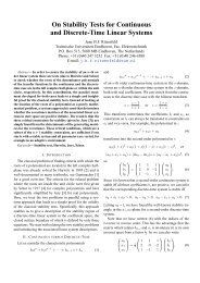
For DF2, K and W can be given in closed form [1]:<br />
( )<br />
1 − b a<br />
a 1 − b<br />
K =<br />
(3)<br />
(1 + b)(1 − a − b)(1 + a − b)<br />
and W has entries<br />
W 11 = (1 − b)(c2 1 + c2 2 ) + 2ac 1c 2<br />
(1 + b){(1 − b) 2 − a 2 } , W 22 = b 2 W 11 + c 2 2<br />
W 12 = W 21 = ab(c2 1 + c2 2 ) + (1 − a2 − b 2 )c 1 c 2<br />
(1 + b)(1 − a − b)(1 + a − b) , (4)<br />
where c 1 and c 2 are the elements of C = (e+ad, f +bd).<br />
Note, incidentally, that W 11 is just equal to the quadratic<br />
form CKC t , and that W 22 can also be written as W 11 −<br />
{(1 − b)c 1 + ac 2 } 2 /{(1 − b) 2 − a 2 }, so W 22 ≤ W 11 .<br />
<strong>The</strong> <strong>Direct</strong> <strong>Wave</strong> <strong>Form</strong> arises from a state transformation<br />
(a rotation in the state plane) applied to DF2. It has a<br />
recursive part that is remindful of a wave digital filter [3],<br />
hence the designation. <strong>The</strong> state description follows from<br />
the matrices A , B , C , D of DF2 via a similarity transformation<br />
A w = T −1 AT , B w = ( T −1 B, C)<br />
w = CT and<br />
D w = D, where T is taken as 1 1 −1<br />
2<br />
. We find:<br />
1 1<br />
A w =<br />
( ) (<br />
1 − γ1 −γ 2<br />
1<br />
, B<br />
γ 1 −1 + γ w =<br />
2 −1<br />
C w = (η 1 − γ 1 d, η 2 − γ 2 d) and D w = (d), (5)<br />
where γ 1 = 1 2 (1 − a − b), γ 2 = 1 2<br />
(1 + a − b), and where<br />
η 1 = 1 2 (d + e + f), η 2 = 1 2<br />
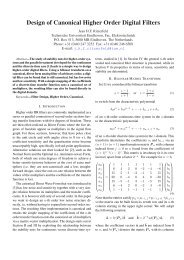
(d − e + f). Fig. 1 depicts<br />
the <strong>Direct</strong> <strong>Wave</strong> <strong>Form</strong>, which is as yet unscaled and uses<br />
only five multipliers directly related to the five coefficients<br />
of H(z), as does the <strong>Direct</strong> <strong>Form</strong>. Incidentally, apart from<br />
a factor 1 2<br />
, the γ’s are simply found from evaluating the<br />
denominator of H(z) at z = ±1, whereas the η’s are found<br />
from the numerator at z = ±1.<br />
In order to L 2 -scale the DWF, we need to calculate its<br />
controllability matrix, which proves to be diagonal:<br />
( )<br />
4γ2 0<br />
0 4γ<br />
K w = T −1 KT −t 1<br />
=<br />
4γ 1 γ 2 (2 − γ 1 − γ 2 ) , (6)<br />
where the denominator is the same as that of K in (3), as<br />
governed by the stability triangle of a <strong>Direct</strong> <strong>Form</strong> in the<br />
(a, b)-plane: 1+b > 0, 1−a−b > 0, 1+a−b > 0. For the<br />
DWF, the region of linear stability is also a triangle in the<br />
(γ 1 , γ 2 )-plane given by: γ 1 > 0, γ 2 > 0, 2−γ 1 −γ 2 > 0.<br />
In Fig. 2 the L 2 -scaled DWF is drawn, where two extra<br />
multipliers 1/ √ K w11 and 1/ √ K w 22 are introduced.<br />
)<br />
,<br />
✲<br />
✻<br />
z −1 ✛ ❄<br />
s 1 [n] ✛<br />
♥+<br />
❄<br />
❆ ✁<br />
❄<br />
✻ η 1 ❆<br />
✁<br />
❆ ✁<br />
❆✁<br />
❆ ✁ −γ 1<br />
❆✁<br />
x[n] ❄<br />
✲ ♥+<br />
✲ ❍ ❍<br />
❄y[n]<br />
✲ d ❍✟ ✲ ♥+ ✲<br />
✻<br />
✟ ✻<br />
✁❆<br />
✁<br />
✁<br />
❆ −γ 2<br />
❆<br />
✻<br />
z −1 ✛ ✟✟✟ ❍ ✛ + ♥ ❄ η 2<br />
✁ ✁✁❆ ❆<br />
s 2 [n] ✛ −1<br />
❆<br />
❍<br />
✻<br />
❄<br />
✻<br />
✲<br />
✲<br />
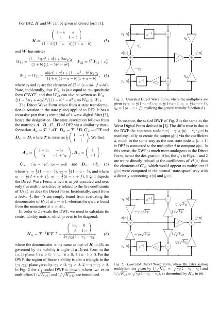
Fig. 1. Unscaled <strong>Direct</strong> <strong>Wave</strong> <strong>Form</strong>, where the multipliers are<br />
given by γ 1 = 1 2 (1−a−b), γ 2 = 1 2 (1+a−b), η 1 = 1 2 (d+e+f),<br />
η 2 = 1 2<br />
(d − e + f), realizing the general transfer function (1).<br />
In essence, the scaled DWF of Fig. 2 is the same as the<br />
<strong>Wave</strong> <strong>Digital</strong> <strong>Form</strong> derived in [1]. <strong>The</strong> difference is that in<br />
the DWF the non-state node x[n] − γ 1 s 1 [n] − γ 2 s 2 [n] is<br />
used explicitly to create the output y[n] via the coefficient<br />
d, much in the same way as the non-state node s 1 [n + 1]<br />
in DF2 is connected to the multiplier d to compute y[n]. In<br />
this sense, the DWF is much more analogous to the <strong>Direct</strong><br />
<strong>Form</strong>, hence the designation. Also, the η’s in Figs. 1 and 2<br />
are more directly related to the coefficients of H(z) than<br />
the elements of C w , which would appear as multipliers if<br />
y[n] were computed in the normal ‘state-space’ way with<br />
d directly connecting x[n] and y[n].<br />
✲<br />
✻<br />
z −1 ✛ ❄<br />
s 1 [n] ✛<br />
♥+<br />
❄<br />
√ ❆ ✁<br />
❄<br />
✻ η 1 k11 ❆<br />
✁<br />
❆ ✁ √ ❆✁<br />
❆ ✁ −γ<br />
❆✁<br />
1 k11<br />
✁ ✁✁❆ ❆1/ √ k 11 ❆<br />
x[n] ❄<br />
✻<br />
✲ ♥+<br />
✲ ❍ ❍<br />
❄y[n]<br />
✲ d ❍✟ ✲ ♥+ ✲<br />
✻<br />
✟ ❄<br />
✻<br />
✁❆<br />
√<br />
✁<br />
✁<br />
❆<br />
❆ ✁<br />
−γ 2 k22 ❆<br />
✁ 1/ √ k 22<br />
❆<br />
❆✁<br />
√<br />
✻<br />
z −1 ✛ ✟✟✟ ❍ ✛ + ♥ ❄ η 2 k22<br />
✁ ✁✁❆ ❆<br />
s 2 [n] ✛ −1<br />
❆<br />
❍<br />
✻<br />
❄<br />
✻<br />
✲<br />
✲<br />
Fig. 2. L 2 -scaled <strong>Direct</strong> <strong>Wave</strong> <strong>Form</strong>, where the extra scaling<br />
multipliers are given by 1/ √ K 11 = √ γ 1 (2 − γ 1 − γ 2 ) and<br />
1/ √ K 22 = √ γ 2 (2 − γ 1 − γ 2 ), as determined by K w in (6).<br />
✲<br />
✲