The Direct Wave Form Digital Filter Structure - Signal Processing ...
The Direct Wave Form Digital Filter Structure - Signal Processing ...
The Direct Wave Form Digital Filter Structure - Signal Processing ...

Create successful ePaper yourself
Turn your PDF publications into a flip-book with our unique Google optimized e-Paper software.
A few remarks on this result are in order: σ 1 and σ 2 are<br />
given in terms of γ 1 and γ 2 , instead of a and b, as are all the<br />
scaling parameters for the DWF (Figs. 2 and 3). Here, this<br />
is particularly useful because the conditions 2ρ > γ 1,2 are<br />
best viewed in the (γ 1 , γ 2 )-plane, where we already have<br />
the stability triangle γ 1 > 0, γ 2 > 0, 2−γ 1 −γ 2 > 0 with<br />
angular points (0, 0), (2, 0) and (0, 2). <strong>The</strong> boundary case<br />
2ρ = γ 2 can also be written as γ 1 = (1 − 1 2 γ 2) 2 , which is<br />
a parabola with tangent lines γ 1 =0 and γ 1 +γ 2 =1 (ρ=0)<br />
touching in (0, 2) and (1, 0), respectively. Likewise, the<br />
boundary 2ρ = γ 1 is the parabola γ 2 = (1 − 1 2 γ 1) 2 , with<br />
tangent lines γ 2 =0 and γ 1 + γ 2 =1 touching in (2, 0) and<br />
(0, 1), respectively. <strong>The</strong>se parabolas mark the transition of<br />
the amplitude responses |F 1,2 (e jϑ )| from having their maximum<br />
at the frequency edges ϑ = 0 or π to some intermediate<br />
frequency. And indeed, as we would expect from the<br />
latter, the region 2ρ > max(γ 1 , γ 2 ), where the left-hand<br />
sides of (18) and (19) hold, is roughly equal to the region<br />
of complex poles (2−γ 1 −γ 2 ) 2 > 4γ 1 γ 2 , or −b > a 2 /4.<br />
Note, that in this region ρ = √ −b is just the pole radius.<br />
✲<br />
✻<br />
z −1 ✛ ❄<br />
s 1 [n] ✛<br />
♥+<br />
❄<br />
❄<br />
✻ η ❆ ✁ 1 σ 1<br />
❆<br />
✁<br />
❆✁<br />
✁ ✁✁❆ ❆✁<br />
✁<br />
−γ 1 σ 1 /σ 3 ❆<br />
σ 3 /σ 1<br />
x[n] ❍ 1/σ 3 ❄<br />
✻<br />
✲ ✲ ♥+<br />
✲ ❍ d σ 3 ❄y[n]<br />
❍ ✲ ❍❍ ✟<br />
✟<br />
✲ ♥+ ✲<br />
✟✟<br />
✻<br />
❄<br />
✟✟<br />
✁❆<br />
❆<br />
✻<br />
✁<br />
−γ 2 σ 2 /σ 3<br />
✁<br />
❆<br />
❆✁<br />
σ 3 /σ 2<br />
✻<br />
z −1 ✛ ✟✟ ✟<br />
❍❍ ✛ + ♥ ❄ η 2 σ 2<br />
✁ ✁✁❆ ❆<br />
s 2 [n] ✛ −1<br />
❄<br />
❍<br />
✻<br />
✻<br />
✲<br />
✲<br />
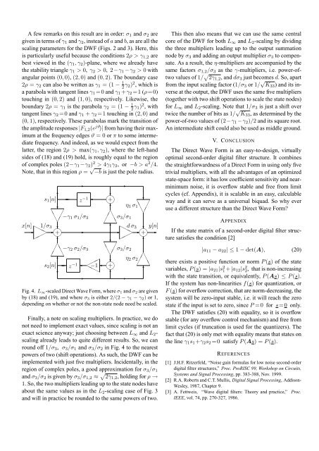
Fig. 4. L ∞ -scaled <strong>Direct</strong> <strong>Wave</strong> <strong>Form</strong>, where σ 1 and σ 2 are given<br />
by (18) and (19), and where σ 3 is either 2/(2 − γ 1 − γ 2 ) or 1,<br />
depending on whether or not the non-state node need be scaled.<br />
Finally, a note on scaling multipliers. In practice, we do<br />
not need to implement exact values, since scaling is not an<br />
exact science anyway; just choosing between L ∞ and L 2 -<br />
scaling already leads to quite different results. So, we can<br />
round off 1/σ 3 , σ 3 /σ 1 and σ 3 /σ 2 in Fig. 4 to the nearest<br />
powers of two (shift operations). As such, the DWF can be<br />
implemented with just five multipliers. Incidentally, in the<br />
region of complex poles, a good approximation for σ 3 /σ 1<br />
and σ 3 /σ 2 is given by σ 3 /σ 1,2 ≈ √ 2γ 1,2 , holding for ρ →<br />
1. So, the two multipliers leading up to the state nodes have<br />
about the same values as in the L 2 -scaling case of Fig. 3<br />
and will in practice be rounded to the same powers of two.<br />
✲<br />
This then also means that we can use the same central<br />
core of the DWF for both L ∞ and L 2 -scaling by dividing<br />
the three multipliers leading up to the output summation<br />
node by σ 3 and adding an output multiplier σ 3 to compensate.<br />
As a result, the η-multipliers are accompanied by the<br />
same factors σ 1,2 /σ 3 as the γ-multipliers, i.e. power-oftwo<br />
values of 1/ √ 2γ 1,2 , and dσ 3 just becomes d. So, apart<br />
from the input scaling factor (1/σ 3 or 1/ √ K 33 ) and its inverse<br />
at the output, the DWF uses the same five multipliers<br />
(together with two shift operations to scale the state nodes)<br />
for L ∞ and L 2 -scaling. Note that 1/σ 3 is just a shift over<br />
twice the number of bits as 1/ √ K 33 , as determined by the<br />
power-of-two values of (2−γ 1 −γ 2 )/2 and its square root.<br />
An intermediate shift could also be used as middle ground.<br />
V. CONCLUSION<br />
<strong>The</strong> <strong>Direct</strong> <strong>Wave</strong> <strong>Form</strong> is an easy-to-design, virtually<br />
optimal second-order digital filter structure. It combines<br />
the straightforwardness of a <strong>Direct</strong> <strong>Form</strong> in using only five<br />
trivial multipliers, with all the advantages of an optimized<br />
state-space form: it has low coefficient sensitivity and nearminimum<br />
noise, it is overflow stable and free from limit<br />
cycles (cf. Appendix), it is scalable in an easy, calculable<br />
way and it can serve as a universal biquad. So why ever<br />
use a different structure than the <strong>Direct</strong> <strong>Wave</strong> <strong>Form</strong>?<br />
APPENDIX<br />
If the state matrix of a second-order digital filter structure<br />
satisfies the condition [2]<br />
|a 11 − a 22 | ≤ 1 − det(A), (20)<br />
there exists a positive function or norm P (s) of the state<br />
variables, P (s) = |a 21 |s 2 1 +|a 12|s 2 2 , that is non-increasing<br />
with the state transition, or equivalently, P (As) ≤ P (s).<br />
If the system has non-linearities f(s) for quantization, or<br />
F (s) for overflow correction, that are norm-decreasing, the<br />
system will be zero-input stable, i.e. it will reach the zero<br />
state if the input is set to zero, since P =0 for s=0 only.<br />
<strong>The</strong> DWF satisfies (20) with equality, so it is overflow<br />
stable (for any overflow control mechanism) and free from<br />
limit cycles (if truncation is used for the quantizers). <strong>The</strong><br />
fact that (20) is only met with equality means that states on<br />
the line γ 1 s 1 +γ 2 s 2 =0 satisfy P (As) = P (s).<br />
REFERENCES<br />
[1] J.H.F. Ritzerfeld, “Noise gain formulas for low noise second-order<br />
digital filter structures,” Proc. ProRISC 99, Workshop on Circuits,<br />
Systems and <strong>Signal</strong> <strong>Processing</strong>, pp. 383-388, Nov. 1999.<br />
[2] R.A. Roberts and C.T. Mullis, <strong>Digital</strong> <strong>Signal</strong> <strong>Processing</strong>, Addison-<br />
Wesley, 1987, Chapter 9.<br />
[3] A. Fettweis, “<strong>Wave</strong> digital filters: <strong>The</strong>ory and practice,” Proc.<br />
IEEE, vol. 74, pp. 270-327, 1986.