The Direct Wave Form Digital Filter Structure - Signal Processing ...
The Direct Wave Form Digital Filter Structure - Signal Processing ...
The Direct Wave Form Digital Filter Structure - Signal Processing ...

Create successful ePaper yourself
Turn your PDF publications into a flip-book with our unique Google optimized e-Paper software.
and similarly, W w of the DWF becomes diagonal:<br />
W w = T t W T =<br />
d 2 ( )<br />
γ1 0<br />
. (14)<br />
2 − γ 1 − γ 2 0 γ 2<br />
<strong>The</strong> noise gain is then G w = 2d 2 /(1 + b) 2 . So, if we take<br />
d = 1 2<br />
(1+b) to make a bandpass filter with maximum amplitude<br />
unity at center frequency ϑ = arccos{a/(1 − b)}<br />
(cf. Section II), its noise gain and its second-order modes<br />
are 1 2<br />
. <strong>The</strong> same values hold for the bandstop function (7),<br />
whereas the allpass filter (8) has second-order modes unity<br />
and noise gain 2, since we need to take d = −(1 + b). <strong>The</strong><br />
fact that the noise gain of these filters does not depend on<br />
the pole angles is very remarkable. Even at extreme angles<br />
the noise behaviour of the DWF stays the same, whereas<br />
<strong>Direct</strong> <strong>Form</strong>s become increasingly noisy.<br />
IV. L ∞ -SCALING OF THE DWF<br />
It is important to realize that L 2 -scaling only guarantees<br />
that the state variables in a system have the same variance<br />
as the input signal, so it is a statistical scaling measure: a<br />
low probability of state overflow is ensured only if the input<br />
signal is sufficiently arbitrary (random) and wide-band,<br />
because the variance is determined by the average power<br />
spectrum. If we know the input signal to be narrow-band<br />
or even sinusoidal at varying frequencies (all of course depending<br />
on the specific application), we must normalize<br />
the two frequency responses F 1,2 (e jϑ ) from input to state<br />
to unity at their maximum amplitudes. This is known as<br />
L ∞ -scaling, denoted as ‖F 1,2 ‖ ∞ = max ϑ |F 1,2 (e jϑ )| = 1.<br />
L ∞ -scaling is more conservative than L 2 -scaling, since it<br />
can be shown that ‖F ‖ ∞ ≥ ‖F ‖ 2 . As an example, let us<br />
look at the transfer function F 3 (z) from the input of the<br />
DWF to its non-state node<br />
F 3 (z) = z2 − 1<br />
z 2 − az − b , (15)<br />
which we have already seen to have a maximum amplitude<br />
response of 2/(1 + b). Calculating its L 2 -norm with<br />
∫ π<br />
−π |F 3(e jϑ )| 2 dϑ results in ‖F 3 ‖ 2 = √ 2/(1 + b), so<br />
√ 1<br />
2π<br />
‖F 3 ‖ ∞ = 2<br />
1 + b<br />
√<br />
2<br />
≥ ‖F 3 ‖ 2 =<br />
1 + b . (16)<br />
If we were to scale the non-state node, we would need<br />
to precede it with a multiplier having the inverse values of<br />
(16) for either L ∞ or L 2 -scaling. <strong>The</strong> question of course is:<br />
would it not be prudent (or even necessary) to do so? Although<br />
it is common practice to use extra bits (double precision)<br />
for the summation nodes as compared to the state<br />
variables, it may take quite a few bits to accommodate the<br />
large signals that would result from b close to −1 (i.e. poles<br />
close to the unit circle). So, to answer the question: it all<br />
depends on whether there are enough bits available for the<br />
non-state summation node in a specific design.<br />
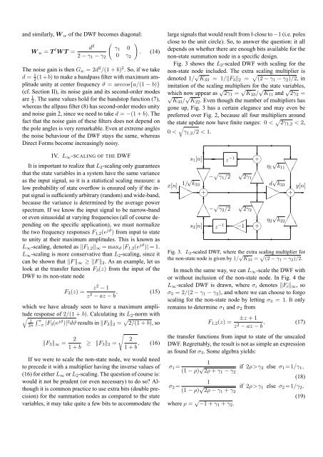
Fig. 3 shows the L 2 -scaled DWF with scaling for the<br />
non-state node included. <strong>The</strong> extra scaling multiplier is<br />
denoted 1/ √ K 33 = 1/‖F 3 ‖ 2 = √ (2 − γ 1 − γ 2 )/2, in<br />
imitation of the scaling multipliers for the state variables,<br />
which now appear as √ 2γ 1 = √ K 33 / √ K 11 and √ √<br />
2γ 2 =<br />
K33 / √ K 22 . Even though the number of multipliers has<br />
gone up, Fig. 3 has a certain elegance and may even be<br />
preferred over Fig. 2, because all four multipliers around<br />
the state update now have finite ranges: 0 < √ 2γ 1,2 < 2,<br />
√<br />
0 < γ 1,2 /2 < 1.<br />
✲<br />
✻<br />
z −1 ✛ ❄<br />
s 1 [n] ✛<br />
♥+<br />
❄<br />
√ ❆ ✁<br />
❄<br />
✻ η 1 k11<br />
❆<br />
✁<br />
❆✁<br />
✁ ✁✁❆ ❆✁<br />
✁<br />
❆ x[n] 1/ √ − √ √<br />
γ 1 /2 2γ1<br />
k<br />
❄<br />
✻<br />
✲ ✲ ♥+<br />
✲ ❍ d √ k<br />
❍ 33 33<br />
❄y[n]<br />
❍ ✲ ❍❍ ✲<br />
✟<br />
✟<br />
♥+ ✲<br />
✟<br />
✟<br />
✻<br />
❄<br />
✻<br />
✁❆<br />
✁<br />
❆<br />
✁<br />
− √ √<br />
γ 2 /2 2γ2<br />
❆<br />
❆✁<br />
√<br />
✻<br />
z −1 ✛ ✟✟ ✟<br />
❍❍ ✛ + ♥ ❄ η 2 k22<br />
✁ ✁✁❆ ❆<br />
s 2 [n] ✛ −1<br />
❄<br />
❍<br />
✻<br />
✻<br />
✲<br />
✲<br />
Fig. 3. L 2 -scaled DWF, where the extra scaling multiplier for<br />
the non-state node is given by 1/ √ K 33 = √ (2 − γ 1 − γ 2 )/2.<br />
In much the same way, we can L ∞ -scale the DWF with<br />
or without inclusion of the non-state node. In Fig. 4 the<br />
L ∞ -scaled DWF is drawn, where σ i denotes ‖F i ‖ ∞ , so<br />
σ 3 = 2/(2 − γ 1 − γ 2 ), and where we can choose to forgo<br />
scaling for the non-state node by letting σ 3 = 1. It only<br />
remains to determine σ 1 and σ 2 from<br />
✲<br />
F 1,2 (z) = ±z + 1<br />
z 2 − az − b , (17)<br />
the transfer functions from input to state of the unscaled<br />
DWF. Regrettably, the result is not as simple an expression<br />
as found for σ 3 . Some algebra yields:<br />
1<br />
σ 1 =<br />
(1 − ρ) √ if 2ρ>γ 2 else σ 1 =1/γ 1 ,<br />
2ρ + γ 1 − γ 2<br />
(18)<br />
1<br />
σ 2 =<br />
(1 − ρ) √ if 2ρ>γ 1 else σ 2 =1/γ 2 ,<br />
2ρ − γ 1 + γ 2<br />
where ρ = √ −1 + γ 1 + γ 2 .<br />
(19)