Rate Adaptation in Time Varying Channels using Acknowledgement ...

More documents

Recommendations

Info

and information outages defined throughout this paper are achievable. The complex channel h k , with variance σh 2 , is time invariant for each packet but varies across packets. The noise vector n k ∈ C N is AWGN with variance σn. 2 If a packet is not received correctly, an outage is said to occur. Practically, this information is available at the receiver via a cyclic redundancy check (CRC) at the medium access control (MAC) layer. The packet is either discarded or re-transmitted later in non-delay sensitive applications. The present packet therefore fails to deliver the data bits and the instantaneous throughput is zero. Otherwise, if the packet is received correctly, the instantaneous throughput, in bit/symbols, equals the data rate. The throughput for the k th packet is therefore defined as T (¯γ,R k ,h k )=R k × (1 − ɛ(¯γ|R k ,h k )) (2) where ɛ(¯γ|R k ,h k ) is the outage probability at an average SNR ¯γ = σ 2 h σ2 x/σ 2 n for a given R k and h k . The actual outage probability function depends on the error correction code used. We treat every K packets as one basic unit: a K-packet. The throughput of a K-packet system with average SNR ¯γ can be generally defined as T K (¯γ,r K , h K )= 1 K K∑ T (¯γ,R k ,h k ) (3) k=1 where h K =[h 1 h 2 ···h K ] and the rate vector is given by r K =[R 1 R 2 ···R K ].TherateR k determines the throughput of packet k as reflected in (3). Interesting, the rate also affects the ability of the transmitter to observe the channel, or CSI, via the ACK feedback - this will become apparent in the next section. III. THROUGHPUT CAPACITY A. Full Channel State Information (CSI) We are interested in maximizing the average throughput of (3) using a packet-by-packet rate adaption scheme. The throughput capacity, or the maximum throughput achievable over the joint distribution of the rate and channel, is defined as CT K [ ,full CSI(¯γ) = sup E rK,h K T K (¯γ,r K , h K ) ] p(r K,h K) [ = sup E rK,h K T K (¯γ,r K , h K ) ] (4) p(r K|h K) where E is the expectation operator (over the distribution given by its subscript). Here, for full generality, we assume that the rate is a random variable for which we want to find the optimal distribution. The second line follows since p(r K , h K )=p(r K |h K )p(h K ) and p(h K ) is related to the channel and is not a parameter available for maximization. It turns out that to achieve the throughput capacity without any restriction, full CSI via h K is required at the transmitter. In practice, full CSI is not available, and also there is a delay in obtaining the CSI. A more general definition for the case that a partial CSI is known at the transmitter follows. B. Partial CSI In general, we want to maximize the throughput using rate adaption given a partial channel knowledge expressed as a random parameter a (which can be discrete or continuous, scalar or vector). The distribution available for maximization is therefore restricted to p(r K |a). However, we now need to take into account the extra random variable a in performing the expectation in (4). This gives us the throughput capacity CT K [ (¯γ) = sup E rK,h K,a T K (¯γ,r K , h K ) ] . (5) p(r K|a) This formulation reduces to (4) when a = h K . The case when no channel knowledge is available can be treated by letting a be an empty vector in (5). The special case when the channel is constant over K packets can be treated by setting h k = h for all k, which is considered in [8]. We now consider the case of interest here in using (5). In the MAC protocol, the simplest feedback provided is via a ACK or negative ACK, i.e. NACK. This is a form of partial CSI. Specifically, denote the CSI of packet k as A k with value 1 for ACK and 0 for NACK. Their probabilities are p(A k =1|R k ,h k )=1− ɛ(¯γ|R k ,h k ), (6) p(A k =0|R k ,h k )=ɛ(¯γ|R k ,h k ). (7) Obviously, A k is dependent on R k , since if R k is large, the possibility of A k =0is high. For the ARQ system, we can replace a in (5) by the ACK vector a K−1 , where we denote a k−1 [a k−2 ,A k−1 ],k = 2, 3, ··· , and a 0 is an empty vector. On the other hand, not all of the ACKs and rates are always available for rate adaptation due to a causality constraint. The information available at packet k is only a k−1 and r k−1 .Tobe exact, R k should then be written explicitly as 2 R k (a k−1 , r k−1 ) when substituting (3) into (5). Similarly, the rate vector should be understood as dependent on the the past ACKs and rates, in the form of r k (a k−1 , r k−1 ). However, the argument will be dropped when there is no ambiguity. IV. GLOBAL OPTIMIZATION A global optimization approach is required to realize (5) which can be re-written using Bayes’ rule as CT K (¯γ) (8) [ = sup E aK−1 E rK|a K−1 E hK|a K−1,r K−1 T K (¯γ,r K , h K ) ] . p(r K|a K−1) It is shown in [8] that the optimal rate for packet k, denoted as Rk o, is deterministic, but still depends on a k−1. Since A k has two possibilities, i.e. |A| =2, then there exist ∑ K−1 k=0 |A|k = 2 K − 1 distinct rates to account for all possible a K−1 .The rate being deterministic has two implications. First, we need to perform a joint maximization over just one modified rate vector containing all possible rates, say r all , rather than over 2 Strictly speaking, R k is a random variable and should not be written as a function of other variables. We stick to this notation for conciseness. We show later that the optimal rate is indeed a deterministic function.
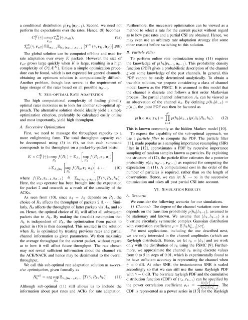
a conditional distribution p(r K |a K−1 ). Second, we need not perform the expectations over the rates. Hence, (8) becomes CT K (¯γ)=sup Tave(¯γ,r K all ), (9a) r all Tave(¯γ,r K [ all )E aK−1 E hK|a K−1,r K−1 T K (¯γ,r K , h K ) ] .(9b) The global solution can be computed off-line and used for rate adaptation over every K packets. However, the size of r all grows large quickly when K is large, resulting in a high complexity of O(|A| K ). Unless a simple optimization procedure can be found, which is not expected for general channels, obtaining an optimum solution is computationally difficult. Another problem, though less severe, is the requirement of large storage of the rates based on all possible a K−1 . V. SUB-OPTIMAL RATE ADAPTATION The high computational complexity of finding globally optimal rates motivates us to look for another sub-optimal approach. The alternative solution should ideally yield a simple optimization criterion, preferably be calculated easily online and most importantly, yield high throughput. A. Successive Optimization First, we need to massage the throughput capacity to a more enlightening form. The total throughput capacity can be decomposed using (3) in (9), so that each summand corresponds to the throughput on a packet-by-packet basis: [ ] K × CT K (¯γ)=sup f(R 1 )+E A1 sup f(R 2 , r 1 , a 1 ) R 1 R 2 ] +E A2|a 1 [sup f(R 3 , r 2 , a 2 ) + ··· (10) R 3 where f(R k , r k−1 , a k−1 ) E hk |r k−1 ,a k−1 [T (¯γ,R k ,h k )]. Here, the sup operator has been brought into the expectation for packet 2 and onwards as a result of the causality of the ACKs. As seen from (10), since a 1 = A 1 depends on R 1 ,the choice of R 1 affects the throughput of packets 2, 3, ···. Similarly, R 2 affects the throughput of latter packets via A 2 , and so on. Hence, the optimal choice of R k will affect all subsequent packets due to A k . By making the (invalid) assumption that A k is independent of R k , the optimization from packet to packet in (10) is then decoupled. This resulted in the solution when R k is optimized by treating previous rates and partial channel information as given parameters. We then maximize the average throughput for the current packet, without regard as to how it will affect future throughput. The rate chosen may not reveal sufficient information about the channel via the ACK/NACK and hence may be detrimental to the overall throughput. We call this sub-optimal rate adaptation solution as successive optimization, given formally as R sub k =argsup R k E hk |a k−1 ,r k−1 [T (¯γ,R k ,h k )] . (11) Although sub-optimal (11) still allows us to include the information about past rates and ACKs for rate adaptation. Furthermore, the successive optimization can be viewed as a method to select a rate for the current packet without regard as to how past rates and a partial CSI are obtained. Hence, we may even use an arbitrary rate adaptation strategy (for some other reason) before switching to this solution. B. Particle Filter To perform online rate optimization using (11) requires the knowledge of p(h k |r k−1 , a k−1 ). This probability density function (PDF) gives a probabilistic description of the channel given some knowledge of the past channels. In general, this PDF cannot be easily determined analytically. To obtain a tractable solution, we propose considering a class of channel model known as the FSMC. It is assumed in this model that the channel is discrete and follows a first order Markovian process. The partial channel information A k can be viewed as an observation of the channel h k . By defining p(h 1 |h −1 )= p(h 1 ), the joint PDF can then be factored as p(h K , a K |r K )= K∏ p(h k |h k−1 )p(A k |R k ,h k ). (12) k=1 This is known commonly as the hidden Markov model [10]. To expose the capability of the sub-optimal approach, we use a particle filter to compute the PDF. The particle filter [11], made popular as a sampling importance resampling (SIR) filter in [12], approximates a PDF by recursive importance sampling of random samples known as particles. By exploiting the structure of (12), the particle filter estimates the a posterior probability p(h k |a K−1 , r K−1 ) as required for computing the expectation in (11). A computational cost in the order of the number of particles is required, rather than on the length of observations. Hence, we can let K →∞in the successive optimization and takes all past partial CSI into account. VI. SIMULATION RESULTS A. Scenario We consider the following scenario for our simulations. 1) Channel: The degree of the channel variation over time depends on the transition probability p(h k |h k−1 ), assumed to be stationary and known. We assume that (h k ,h k−1 ) is a bivariate circularly symmetric complex Gaussian distribution with correlation coefficient ρ = E[h k h ∗ k−1 ]/σ2 h . For most applications, including the one described next, we are only interested in the channel amplitudes (which are Rayleigh distributed). Hence, we let r k = |h k | and we work only with the distribution of r k using the FSMC [9]. Furthermore, we approximate the channel r k using discrete values from 0 to 5 in steps of 0.01, which is experimentally found to be have sufficient accuracy in representing the channel when ¯γ =0dB. At other SNR, the instantaneous SNR is scaled accordingly so that we can still use the same Rayleigh PDF with ¯γ =0dB. The bivariate rayleigh PDF and the cumulative distribution function (CDF) of (r k ,r k−1 ) can be specified by E[r the power correlation coefficient ρ r 2 = 2 k r2 k−1 √ ] The E[r 4 k ]E[rk−1 4 ]. CDF is represented as a power series in [13] for the Rayleigh
Page 1: Rate Adaptation in Time Varying Cha
Page 5: Throughput 5 4.8 4.6 4.4 4.2 4 3.8

Rate Adaptation in Time Varying Channels using Acknowledgement ...

You also want an ePaper? Increase the reach of your titles

Delete template?

Save as template?