analysis of the rts/cts multiple access scheme with capture effect
analysis of the rts/cts multiple access scheme with capture effect
analysis of the rts/cts multiple access scheme with capture effect

Create successful ePaper yourself
Turn your PDF publications into a flip-book with our unique Google optimized e-Paper software.
The 17th Annual IEEE International Symposium on Personal, Indoor and Mobile Radio Communications (PIMRC’06)<br />
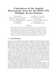
ANALYSIS OF THE RTS/CTS MULTIPLE ACCESS SCHEME<br />
WITH CAPTURE EFFECT<br />
Chin Keong Ho †§<br />
†Eindhoven University <strong>of</strong> Technology<br />
Eindhoven, The Ne<strong>the</strong>rlands<br />
Jean-Paul M. G. Linnartz §†<br />
§Philips Research Laboratories<br />
Eindhoven, The Ne<strong>the</strong>rlands<br />
ABSTRACT<br />
The Request-to-Send (RTS) / Clear-to-Send (CTS) <strong>scheme</strong><br />
uses a four-way handshake to ensure proper spatial and temporal<br />
reservation <strong>of</strong> <strong>the</strong> <strong>multiple</strong>-<strong>access</strong> wireless LAN channel.<br />
By considering <strong>the</strong> (interdependence <strong>of</strong>) successive <strong>capture</strong><br />
probabilities for a cycle <strong>of</strong> an RTS, CTS, data packet and<br />
acknowledgement, we analyze <strong>the</strong> throughput <strong>of</strong> <strong>the</strong> RTS/CTS<br />
<strong>scheme</strong> in a new ma<strong>the</strong>matical framework. We also propose<br />
closed-form bounds which are useful for rate optimization.<br />
I. INTRODUCTION<br />
The performance <strong>of</strong> today’s wireless LANs is increasingly limited<br />
by mutual interference. Several mechanisms are used to<br />
allow co-existence, such as carrier sensing and virtual sensing.<br />
Carrier sensing is a <strong>multiple</strong> <strong>access</strong> <strong>scheme</strong> that inhibits<br />
transmission when an ongoing transmission is detected at <strong>the</strong><br />
transmitter [1]. However, in some situations users are inhibited<br />
unnecessarily [2]. This could be solved by virtual sensing in<br />
which <strong>the</strong> source first asks <strong>the</strong> destination whe<strong>the</strong>r <strong>the</strong> channel<br />
is idle by a Request-to-Send (RTS) packet, and <strong>the</strong> destination<br />
confirms this <strong>with</strong> a Clear-to-Send (CTS) packet [2]. Remote<br />
stations that recover <strong>the</strong> RTS or CTS packet are inhibited to<br />
transmit during some specified time, hence increasing <strong>the</strong> probability<br />
<strong>of</strong> a successful transmission.<br />
Two types <strong>of</strong> model for packet recovery have been assumed<br />
when considering <strong>the</strong> RTS/CTS <strong>scheme</strong>. In <strong>the</strong> collision<br />
model, a packet is correctly received, i.e., recovered, if and<br />
only if <strong>the</strong>re is no o<strong>the</strong>r concurrent transmission, e.g. [3]. A improved<br />
model is based on <strong>the</strong> power <strong>capture</strong> <strong>effect</strong>: a packet is<br />
recovered (even if <strong>the</strong>re are interfering signals) if and only if <strong>the</strong><br />
signal-to-noise plus interference ratio (SINR) is greater than a<br />
<strong>capture</strong> ratio, e.g. [4, 5]. In <strong>the</strong> literature [3, 4, 5], <strong>the</strong> RTS/CTS<br />
<strong>scheme</strong> has been modeled by assuming that if <strong>the</strong> RTS is recovered<br />
by <strong>the</strong> destination, <strong>the</strong>n <strong>the</strong> CTS, payload (PAY) and<br />
acknowledgement (ACK) will be recovered too. This is in fact<br />
an approximation that violates <strong>the</strong> principle <strong>of</strong> <strong>the</strong> <strong>capture</strong> <strong>effect</strong>.<br />
By removing this approximation, <strong>the</strong> causal <strong>effect</strong> <strong>of</strong> <strong>the</strong><br />
RTS, CTS, PAY and ACK in time is analyzed in [6].<br />
This paper extends <strong>the</strong> results <strong>of</strong> [6] by calculating <strong>the</strong><br />
throughput achieved using <strong>the</strong> RTS/CTS <strong>scheme</strong>. By choosing<br />
appropriate RTS, CTS and PAY transmission rates, we illustrate<br />
by numerical examples how throughput maximization<br />
can be carried out. Moreover, by deriving closed-form throughput<br />
lower bounds, it is shown quantitatively that <strong>the</strong> RTS/CTS<br />
<strong>scheme</strong> is superior to <strong>the</strong> ALOHA <strong>scheme</strong> when <strong>the</strong> PAY length<br />
is sufficiently long (such that that <strong>the</strong> overheads are small) and<br />
when <strong>the</strong> RTS and CTS rates are sufficiently small (such that<br />
<strong>the</strong> interference are low).<br />
<br />
<br />
<br />
<br />
<br />
<br />
<br />
<br />
<br />
<br />
<br />
<br />
<br />
<br />
<br />
<br />
<br />
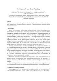
Figure 1: RTS/CTS <strong>multiple</strong> <strong>access</strong> <strong>scheme</strong>.<br />
A. RTS/CTS Scheme<br />
II.<br />
MODEL<br />
<br />
The test station (STA) will be referred to simply as STA and <strong>the</strong><br />
o<strong>the</strong>r STAs as interferers. We assume that STA uses RTS/CTS<br />
for channel <strong>access</strong> to <strong>the</strong> intended destination which we assume<br />
to be <strong>the</strong> <strong>access</strong> point, AP. On <strong>the</strong> o<strong>the</strong>r hand, <strong>the</strong> interferers<br />
use slotted ALOHA for <strong>multiple</strong> <strong>access</strong>.<br />
The detailed RTS/CTS <strong>scheme</strong> considered here is shown in<br />
Fig. 1. A transmission cycle consists <strong>of</strong> an RTS packet, a CTS<br />
packet, a PAY (data) packet and an ACK packet; for conciseness<br />
<strong>the</strong> word “packet” is subsequently omitted when referring<br />
to <strong>the</strong> different packet types. For ease <strong>of</strong> <strong>analysis</strong>, we assume<br />
<strong>the</strong> system to be time slotted. Each RTS, CTS and ACK uses<br />
one slot, and <strong>the</strong> PAY uses P slots. As illustrated, if <strong>the</strong> interferers<br />
recover <strong>the</strong> RTS (CTS), <strong>the</strong>y are inhibited to transmit<br />
during <strong>the</strong> CTS and ACK periods (PAY period, respectivly).<br />
In <strong>effect</strong>, <strong>the</strong> inhibition period is kept to a minimum; this is in<br />
contrast to <strong>the</strong> practice <strong>of</strong> IEEE 802.11, where any inhibition<br />
is carried out continuously until <strong>the</strong> cycle completes. Fur<strong>the</strong>rmore,<br />
we assume:<br />
1) No carrier sensing: In contrast to common practice in<br />
IEEE 802.11, we explicitly do not consider that carrier sensing<br />
is carried out, but only virtual sensing via <strong>the</strong> RTS/CTS mechanism.<br />
This eliminates <strong>the</strong> exposed node problem associated<br />
<strong>with</strong> carrier sensing.<br />
2) Only STA is fully RTS/CTS capable: For analytical<br />
tractability, we assume that only STA uses RTS/CTS for <strong>multiple</strong><br />
<strong>access</strong>. The interferers uses slotted ALOHA. Yet, <strong>the</strong>y<br />
obey <strong>the</strong> RTS/CTS rules, that is, <strong>the</strong>y temporarily refrain from<br />
transmission after <strong>the</strong>y recover any RTS or CTS.<br />
3) Slotted Data Detection: Data is (transmitted and) detected<br />
during PAY on a slot by slot basis, independently <strong>of</strong> o<strong>the</strong>r slots.<br />
As a result, <strong>the</strong> ACK comprises <strong>of</strong> <strong>multiple</strong> acknowledgement<br />
bits, one bit for each slot <strong>of</strong> data. This assumption allows <strong>the</strong><br />
<strong>capture</strong> model to be applied for each slot independently.<br />
1-4244-0330-8/06/$20.00 c○2006 IEEE
The 17th Annual IEEE International Symposium on Personal, Indoor and Mobile Radio Communications (PIMRC’06)<br />
B. Capture, Channel and Network Models<br />
The instantaneous SINR can be represented as<br />
p 0<br />
SINR =<br />
N o + ∑ N<br />
i=1 p , (1)<br />
i<br />
where p 0 , p i is <strong>the</strong> instantaneous signal power <strong>of</strong> STA and <strong>the</strong><br />
i th interferer, respectively, while N o is <strong>the</strong> noise power. From<br />
information <strong>the</strong>ory, when <strong>the</strong> interference and <strong>the</strong> data is independent<br />
Gaussian distributed, an achievable instantaneous<br />
data rate, in bits/symbol, is given by <strong>the</strong> mutual information<br />
I(SINR) = log(1 + SINR). An information outage is said to<br />
occur if <strong>the</strong> instantaneous mutual information is smaller than<br />
R, i.e., when SINR < 2 R − 1.<br />
The <strong>capture</strong> <strong>effect</strong>, channel and network are modeled as follows.<br />
1) Capture Effect: The <strong>capture</strong> <strong>effect</strong> is modeled by assuming<br />
that <strong>the</strong> packet is correctly decoded if and only if <strong>the</strong>re is<br />
no information outage, hence relating <strong>the</strong> <strong>capture</strong> ratio to <strong>the</strong><br />
rate as z(R) 2 R − 1.<br />
2) Path Loss: All transmitters use <strong>the</strong> same power. However,<br />
each signal experiences path loss depending on <strong>the</strong> propagation<br />
distance, a. We model <strong>the</strong> local mean power according to <strong>the</strong><br />
path loss law ¯p = a −β where β = 4 is used in this paper.<br />
3) Channel: Each channel exhibits quasi-static flat Rayleigh<br />
fading during one RTS, CTS, PAY or ACK transmission, but<br />
independent for different transmission links and slots. Hence,<br />
<strong>the</strong> probability density function (pdf) <strong>of</strong> <strong>the</strong> power p is f p (p) =<br />
1<br />
¯p exp (− p¯p<br />
)<br />
.<br />
4) Interferers’ Positions: The x- and y-coordinates <strong>of</strong> <strong>the</strong><br />
STA and AP are denoted by position vectors a STA , a AP , respectively.<br />
When <strong>the</strong> RTS/CTS <strong>scheme</strong> is not implemented,<br />
interfering packets are transmitted according to a homogenous<br />
(spatial) Poisson process <strong>with</strong> intensity G(a) = G o packets per<br />
time slot per unit area, where 0 < G o < ∞ and a is in an operating<br />
region A. The total traffic rate is G t = ∫ G(a) da.<br />
a∈A<br />
In this paper, we let <strong>the</strong> region A grows infinitely large.<br />
III.<br />
CAPTURE PROBABILITY<br />
Consider a source at a source transmitting a packet <strong>of</strong> length L<br />
and rate R to a destination at a dest . The traffic intensity is G(a).<br />
The event that <strong>the</strong> packet is recovered, i.e., that <strong>the</strong> packet <strong>capture</strong>s<br />
<strong>the</strong> receiver, is denoted as E cap (a source , a dest , R, L, G).<br />
The arguments <strong>of</strong> z and E cap will be dropped when <strong>the</strong>re is no<br />
ambiguity.<br />
A. General Capture Probability<br />
Let f pi denote <strong>the</strong> (exponential) pdf <strong>of</strong> <strong>the</strong> power <strong>of</strong> <strong>the</strong> i th<br />
interferer and L f (s) <strong>the</strong> Laplace transform <strong>of</strong> function f evaluated<br />
at s. Define<br />
W (2 R −1, |a source −a dest |, |a i −a dest |) = 1−L fpi ((2 R −1)/¯p).<br />
Then, <strong>the</strong> <strong>capture</strong> probability can be simplified as [7]<br />
{<br />
Pr{E cap } = exp − zN o<br />
¯p<br />
∫a − J (a i ) da i<br />
}, (2)<br />
i∈A<br />
J (a i ) W (z, |a source − a dest |, |a i − a dest |)G(a i ). (3)<br />
B. Data Capture Probability<br />
Let E R , E C , E P and E A respectively denote <strong>the</strong> <strong>capture</strong> events<br />
that a slot <strong>of</strong> <strong>the</strong> RTS, CTS, PAY and ACK are recovered. Note<br />
that for P > 1, E P is <strong>the</strong> <strong>capture</strong> event <strong>of</strong> a given slot during<br />
PAY, but is statistically <strong>the</strong> same for any slot due to <strong>the</strong> assumption<br />
that <strong>the</strong> channel is independent for every slot. The event<br />
that <strong>the</strong> data in a slot carried by <strong>the</strong> PAY is considered to be<br />
transported to <strong>the</strong> destination, denoted as E data , occurs if all<br />
<strong>the</strong> above four <strong>capture</strong> events occurs, since <strong>the</strong> ACK contains<br />
acknowledgement bits for all PAY slots. Hence, <strong>the</strong> probability<br />
that <strong>the</strong> data in a PAY slot is recovered by <strong>the</strong> AP, i.e., <strong>the</strong> data<br />
<strong>capture</strong> probability, can be expressed using <strong>the</strong> chain rule as<br />
Pr(E data ) = Pr(E R , E C , E P , E A )<br />
= Pr(E R ) Pr(E C |E R ) Pr(E P |E R , E C ) Pr(E A |E R , E C , E P ).(4)<br />
Unlike <strong>the</strong> RTS and CTS which inhibits o<strong>the</strong>r users, reducing<br />
<strong>the</strong> ACK rate does not incur any penalty on <strong>the</strong> network. Often,<br />
<strong>the</strong> ACK is transmitted at <strong>the</strong> lowest possible rate to ensure reliable<br />
communication. To make <strong>the</strong> <strong>analysis</strong> concise, we approximate<br />
R A as (<strong>effect</strong>ively) zero and so Pr(E A |E R , E C , E P ) = 1.<br />
Hence, to compute Pr(E data ) <strong>the</strong>n only requires computing <strong>the</strong><br />
first three factors <strong>of</strong> (4).<br />
We use Φ, Θ ∈ {R, C, P, A} to denote a generic packet type.<br />
Fur<strong>the</strong>rmore, E refers to any or some <strong>of</strong> {E R , E C , E P , E A , ∅},<br />
where ∅ denotes a null set. We also use <strong>the</strong> following notations:<br />
1) R Φ is <strong>the</strong> rate used for transmitting Φ;<br />
2) z Φ 2 RΦ − 1 is <strong>the</strong> <strong>capture</strong> ratio;<br />
3) G Φ|E (a) is <strong>the</strong> spatial traffic intensity at a when Φ is transmitted<br />
conditioned on event E; and<br />
4) P Φ|E (a) is <strong>the</strong> probability that Φ <strong>capture</strong>s a receiver at a<br />
conditioned on event E.<br />
Here, <strong>the</strong> position vector a is <strong>the</strong> position <strong>of</strong> an interferer for<br />
<strong>the</strong> traffic intensity or <strong>of</strong> a receiver for <strong>the</strong> <strong>capture</strong> probability.<br />
C. Relationship <strong>of</strong> Traffic Intensity and Capture Probability<br />
Computing any <strong>capture</strong> probability can be carried out using (2)<br />
if <strong>the</strong> traffic intensity is known. Hence, <strong>the</strong> problem <strong>of</strong> finding<br />
<strong>the</strong> <strong>capture</strong> probability is reduced to finding <strong>the</strong> corresponding<br />
traffic intensity. Based on <strong>the</strong> RTS/CTS <strong>scheme</strong> described in<br />
Sect. A., <strong>the</strong> <strong>capture</strong> probability for different packet types at a<br />
is<br />
P R|E (a) = Pr { E cap (a STA , a, R R , G R|E ) } , (5)<br />
P C|E (a) = Pr { E cap ( a AP , a, R C , G C|E ) } , (6)<br />
P P|E (a) = Pr { E cap (a STA , a, R P , G P|E ) } . (7)<br />
The individual <strong>capture</strong> probability <strong>of</strong> (4) can <strong>the</strong>n be expressed<br />
concisely as special cases <strong>of</strong> (5), (6), (7), respectively:<br />
Pr(E R ) = P R (a AP ), (8)<br />
Pr(E C |E R ) = P C|ER (a STA ), (9)<br />
Pr(E P |E R , E C ) = P P|ER,E C<br />
(a AP ). (10)<br />
D. Capture Probabilities Pr(E R ), Pr(E C |E R ), Pr(E P |E R , E C )<br />
We summarized <strong>the</strong> computations required to calculate<br />
Pr(E R ), Pr(E C |E R ), Pr(E P |E R , E C ); details are provided in
The 17th Annual IEEE International Symposium on Personal, Indoor and Mobile Radio Communications (PIMRC’06)<br />
(12)<br />
↦→ G R|ER (a) (5)<br />
−→ P R|ER (a) (13)<br />
−→ G C|ER (a) (6)<br />
−→ P C|ER (a) (9)<br />
−→ Pr(E C |E R )<br />
Figure 2: Relationship <strong>of</strong> <strong>capture</strong> probabilities and traffic intensities over time and space in calculating Pr(E C |E R ).<br />
· · · → G C|ER (a) (14)<br />
−→ G C|ER,E C<br />
(a) (6)<br />
−→ P C|ER,E C<br />
(a) (15)<br />
−→ G P|ER,E C<br />
(a) (7)<br />
−→ P P|ER,E C<br />
(a) (10)<br />
−→ Pr(E P |E R , E C )<br />
Figure 3: Relationship <strong>of</strong> <strong>capture</strong> probabilities and traffic intensities over time and space in calculating Pr(E P |E R , E C ).<br />
[6]. To emphasis <strong>the</strong> effe<strong>cts</strong> <strong>of</strong> interference, we consider <strong>the</strong><br />
case when <strong>the</strong> noise is negligible, i.e., N o = 0.<br />
The RTS <strong>capture</strong> probability can be derived in closed-form<br />
as<br />
Pr(E R ) = exp { −a 2 sπ 2 G o<br />
√<br />
zR /2 } (11)<br />
where a s = |a STA − a AP | is <strong>the</strong> distance between STA and AP.<br />
On <strong>the</strong> o<strong>the</strong>r hand, <strong>the</strong> conditional CTS <strong>capture</strong> probability is<br />
fairly difficult to compute, given by <strong>the</strong> sequence <strong>of</strong> computation<br />
(as time progresses in <strong>the</strong> RTS/CTS cycle) in Fig. 2. To<br />
complete <strong>the</strong> computation, <strong>the</strong> conditional traffic intensities can<br />
be shown to be<br />
G R|ER (a) = G o (1 − W (z R , a s , |a − a AP |)), (12)<br />
G C|ER (a) = G o<br />
(<br />
1 − PR|ER (a) ) . (13)<br />
Similarly, <strong>the</strong> conditional PAY <strong>capture</strong> probability is computed<br />
as shown in Fig. 3 using <strong>the</strong> following conditional traffic<br />
intensities<br />
G C|ER,E C<br />
(a) = (1 − W (z C , a s , |a − a STA |))G C|ER (a),(14)<br />
G P|ER,E C<br />
(a) = G o<br />
(<br />
1 − PC|ER,E<br />
C<br />
(a)) ) . (15)<br />
Note that G C|ER is required to start <strong>the</strong> computation and is available<br />
from Fig. 2.<br />
IV.<br />
LOWER BOUND CAPTURE PROBABILITIES<br />
Closed-form expressions ease optimization studies, specifically<br />
for throughput maximization. Although Pr(E R ) is available<br />
in closed form, exact closed forms for <strong>the</strong> conditional CTS<br />
and PAY <strong>capture</strong> probabilities are not available. Instead, lower<br />
bound closed forms are derived here.<br />
A general approach to lower bound <strong>the</strong> <strong>capture</strong> probability<br />
during Φ is to upper bound <strong>the</strong> corresponding traffic intensity<br />
during Φ. We show that this upper bound traffic intensity can be<br />
obtained by using a uniform upper bound traffic intensity during<br />
Θ where Θ occurs before Φ. By choosing Θ appropriately,<br />
a closed-form for <strong>the</strong> <strong>capture</strong> probability can <strong>the</strong>n be obtained.<br />
All lower bound <strong>capture</strong> probabilities are denoted by capping<br />
<strong>the</strong> exact ones <strong>with</strong> tildes; all upper bound traffic intensities are<br />
denoted similarly.<br />
A. Lower Bound CTS Capture Probability<br />
We proceed in <strong>the</strong> forward time sense as indicated by <strong>the</strong> arrows<br />
in Fig. 2. From (12), a valid upper bound <strong>of</strong> G R|ER (a) is<br />
G o since it can be shown that <strong>the</strong> W function is always positive.<br />
This gives us a lower bound to P R|ER (a), which can be<br />
appreciated by observing <strong>the</strong> relationship <strong>of</strong> <strong>the</strong> <strong>capture</strong> probability<br />
and <strong>the</strong> traffic intensity in (2). Since <strong>the</strong> upper bound<br />
traffic is uniform, <strong>the</strong> lower bound <strong>capture</strong> probability is <strong>the</strong><br />
same as <strong>the</strong> RTS <strong>capture</strong> probability, <strong>the</strong>refore<br />
˜P R|ER (a) = exp { −b 2 π 2 G o<br />
√<br />
zR /2 } (16)<br />
where b = |a STA − a|. From (16) and (13), we <strong>the</strong>n obtain an<br />
upper bound to G C|ER (a) as<br />
˜G C|ER (a) = G o<br />
(1 − ˜P<br />
)<br />
R|ER (a)<br />
(17)<br />
which can be alternatively written as function <strong>of</strong> b, i.e., as<br />
˜G C|ER (b). Using (2) <strong>with</strong> transformation <strong>of</strong> <strong>the</strong> random variable<br />
from a to b, <strong>the</strong> desired lower bound is<br />
{ ∫ ∞<br />
}<br />
˜Pr(E C |E R ) = exp − 2πbW (z C , a s , b) ˜G C|ER (b) db , (18)<br />
0<br />
where noise is assumed to be absent. After some derivations<br />
(omitted due to lack <strong>of</strong> space), we obtain<br />
˜Pr(E C |E R ) = exp{a 2 sπG o<br />
√<br />
zC × g(G o π 2 a 2 s√<br />
zC z R /2)<br />
−a 2 sπ 2 G o<br />
√<br />
zC /2} (19)<br />
where g(s) cos(s) [ π<br />
2 − Si(s)] + sin(s)Ci(s), Si(s) =<br />
∫ π 2 −<br />
∞ sin y<br />
s y<br />
dy is <strong>the</strong> sine integral and Ci(s) = − ∫ ∞ cos y<br />
s y<br />
dy <strong>the</strong><br />
cosine integral.<br />
B. Lower Bound PAY Capture Probability<br />
The lower bound for PAY follows <strong>the</strong> same derivation as that<br />
for CTS. We proceed according to Fig. 3. First we bound<br />
G C|ER,E C<br />
(a) by G o . This is valid as seen from (14) and (13).<br />
Carrying on <strong>the</strong> arguments in a similar way, we arrive at<br />
˜P C|ER,E C<br />
(a) = exp { −b 2 π 2 √<br />
G o zC /2 } , (20)<br />
˜G P|ER,E C<br />
(a) = G o<br />
(1 − ˜P<br />
)<br />
C|ER,E C<br />
(a) , (21)<br />
where b = |a AP − a|. Therefore, similar to <strong>the</strong> derivation <strong>of</strong><br />
(19), <strong>the</strong> <strong>capture</strong> probability for <strong>the</strong> PAY is lower bounded by<br />
˜Pr(E P |E R , E C ) = exp{a 2 sπG o<br />
√<br />
zP · g(G o π 2 a 2 s√<br />
zP z C /2)<br />
A. Analysis<br />
−a 2 sπ 2 G o<br />
√<br />
zP /2}. (22)<br />
V. THROUGHPUT<br />
For <strong>the</strong> purpose <strong>of</strong> <strong>analysis</strong>, we assume that <strong>the</strong> RTS/CTS cycles<br />
are spaced sufficiently far apart so that <strong>the</strong> inhibition period<br />
<strong>of</strong> one cycle do not overlap <strong>with</strong> <strong>the</strong> next . We consider<br />
<strong>the</strong> throughput <strong>of</strong> <strong>the</strong> RTS/CTS <strong>scheme</strong> averaged over <strong>the</strong> time<br />
when STA <strong>access</strong>es <strong>the</strong> channel via RTS/CTS.
The 17th Annual IEEE International Symposium on Personal, Indoor and Mobile Radio Communications (PIMRC’06)<br />
The last line <strong>of</strong> (27) is obtained by using (4) and assuming<br />
Consider <strong>the</strong> possible cases when a cycle is terminated from<br />
where Ω(P ) <br />
P Pr(E R , E C )<br />
2 + (P + 1) Pr(E R , E C ) . (28) ing <strong>the</strong> slotted ALOHA is plotted in Fig. 4. We assumed for<br />
simplicity that ACK is not required for ALOHA and hence<br />
<strong>the</strong> STA’s perspective. There are only two, ei<strong>the</strong>r when (i) STA Pr(E A |E R , E C , E P ) = 1.<br />
does not recover <strong>the</strong> CTS (including <strong>the</strong> case that <strong>the</strong> CTS may<br />
not be sent by <strong>the</strong> AP in <strong>the</strong> first place because <strong>the</strong> RTS is not<br />
recovered), or when (ii) STA has received <strong>the</strong> ACK (but may<br />
not necessarily recover it). These cases are indicated respectively<br />
Property 1 For a given R R , R C , R P , <strong>the</strong> throughput ¯s is an<br />
increasing function <strong>of</strong> P . Hence, an upper bound is given by<br />
<strong>the</strong> asymptotic throughput<br />
as {R, C}, {R, C, P, A}. The first case occurs if <strong>the</strong> RTS<br />
or <strong>the</strong> CTS is not recovered <strong>with</strong> probability<br />
lim P Pr(E P |E R , E C ).<br />
P →∞<br />
(29)<br />
Pr(ĒR) + Pr(E R , ĒC) = 1 − Pr(E R , E C ), (23)<br />
Pro<strong>of</strong> 1 Note that R P Pr(E P |E R , E C ) in (27) is independent<br />
where Ē indicates <strong>the</strong> complement <strong>of</strong> event E. The second case,<br />
<strong>the</strong>refore, occurs <strong>with</strong> probability Pr(E R , E C ).<br />
The duration <strong>of</strong> each cycle <strong>of</strong> <strong>the</strong> RTS/CTS transmission,<br />
<strong>of</strong> P , while as P increases, Ω(P ) increases (hence proving<br />
<strong>the</strong> first statement <strong>of</strong> <strong>the</strong> proposition) and approaches 1 (hence<br />
proving <strong>the</strong> second).<br />
i.e., <strong>the</strong> cycle time, is i.i.d. As a result, <strong>the</strong> cycle time is a<br />
renewal process. Let s t ∈ {0, L sym × R P } be <strong>the</strong> amount <strong>of</strong><br />
bits recovered in slot t, where L sym is <strong>the</strong> number <strong>of</strong> symbols<br />
Property 2 For any given R R , R C , P , <strong>the</strong> optimal R P that<br />
maximizes ¯s is <strong>the</strong> same.<br />
sent per slot. Note that s t can be greater than zero only during<br />
PAY period, o<strong>the</strong>rwise it is zero since only overheads are sent. Pro<strong>of</strong> 2 When R R , R C , P are given, Ω(P ) is independent <strong>of</strong><br />
By using <strong>the</strong> renewal-reward <strong>the</strong>orem [8], <strong>the</strong> time average <strong>of</strong> R P while R P and Pr(E P |E R , E C ) are functions <strong>of</strong> R P . Hence,<br />
<strong>the</strong> throughput in bit/symbol over an infinitely large period is maximizing ¯s is equivalent to maximizing (29), and is independent<br />
<strong>of</strong> <strong>the</strong> actual values <strong>of</strong> R R , R C , P .<br />
1 1<br />
N∑<br />
¯s(a s , R R , R C , R P , P ) lim<br />
s t<br />
N→∞ L sym N<br />
From Properties 1, 2, it follows that for any given R R , R C , <strong>the</strong><br />
t=1<br />
maximum throughput ¯s obtained by optimizing R P increases<br />
1 E [R]<br />
=<br />
(24) <strong>with</strong> P . This is because increasing P reduces <strong>the</strong> overhead and<br />
L sym E [T ]<br />
does not have any negative effe<strong>cts</strong>, which follows intuitively<br />
<strong>with</strong> probability 1. Here, <strong>the</strong> expectation E is carried out over<br />
<strong>the</strong> events in one cycle, R is <strong>the</strong> reward in <strong>the</strong> form <strong>of</strong> <strong>the</strong> sum<br />
<strong>of</strong> s t in a cycle, and T is <strong>the</strong> cycle time in slots. As explicitly<br />
denoted, <strong>the</strong> time averaged throughput is a function <strong>of</strong> many<br />
parameters. We take a s to be fixed, and consider how <strong>the</strong> rates<br />
and PAY length P affect <strong>the</strong> throughput. For notational convenience,<br />
<strong>the</strong> arguments <strong>of</strong> ¯s are dropped.<br />
On average, P Pr(E data ) slots are successful during <strong>the</strong> PAY<br />
period. Hence, <strong>the</strong> expected reward is<br />
from <strong>the</strong> fact that <strong>the</strong> data are detected independently on a slot<br />
by slot basis.<br />
To improve <strong>the</strong> reliability <strong>of</strong> <strong>the</strong> data, <strong>the</strong> lowest practical<br />
rate for R R , R C may be chosen to ensure <strong>the</strong> largest reservation<br />
<strong>effect</strong> over space. However, it may be necessary to reduce <strong>the</strong><br />
amount <strong>of</strong> inhibition, in which case moderate values <strong>of</strong> rates<br />
may be chosen. After R R , R C are fixed, as a consequence <strong>of</strong><br />
Properties 1, 2, we can choose P as large as practically possible<br />
and also independently optimize R P for <strong>the</strong> given R R , R C .<br />
E [R] = L sym R P P Pr(E data ) (25) Property 3 A lower bound <strong>of</strong> ¯s is obtained by substituting <strong>the</strong><br />
Taking into account that <strong>the</strong> cases {R, C}, {R, C, P, A} use 2 <strong>capture</strong> probabilities in (27) <strong>with</strong> <strong>the</strong>ir lower bounds (19), (22).<br />
and P + 3 slots, respectively, <strong>the</strong> expected cycle time is<br />
P<br />
Pro<strong>of</strong> 3 By rewriting Ω(P ) =<br />
2/ Pr(E R,E C)+(P +1)<br />
, we obtain<br />
E [T ] = 2(1 − Pr(E R , E C )) + (P + 3) Pr(E R , E C )<br />
= 2 + (P + 1) Pr(E R , E C ). (26)<br />
P<br />
¯s ≥ ˜s R P˜Pr(EP |E R , E C )<br />
This result can be explained as follows. From (26), it is seen<br />
2/˜Pr(E R , E C ) + (P + 1) . (30)<br />
that at least two slots are used for <strong>the</strong> cycle. This overhead corresponds<br />
to <strong>the</strong> RTS and CTS slot since STA has to wait for <strong>the</strong><br />
B. Numerical Results<br />
CTS to arrive before deciding to transmit PAY or to defer <strong>the</strong> The throughput ¯s vs R P is plotted in Fig. 4. The following system<br />
parameters are fixed: R R = R C = 0.5, a s = 0.5, G o =<br />
transmission. Subsequently, if <strong>the</strong> RTS and CTS are recovered<br />
(<strong>with</strong> probability Pr(E R , E C )), P slots are used for PAY and 1/π, while P are varied. For a fixed P , as R P increases,<br />
one slot for a potential ACK. The potential ACK requires one ¯s increases initially, peaking at some R P , say RP o (P ), <strong>the</strong>n<br />
slot since STA has to spend time receiving <strong>the</strong> ACK regardless decreases. This is because transmitting at a low R P limits<br />
<strong>of</strong> whe<strong>the</strong>r it is actually sent by <strong>the</strong> AP.<br />
<strong>the</strong> throughput, while transmitting at a high R P reduces <strong>the</strong><br />
Using (25) and (26), (24) becomes<br />
throughput as <strong>the</strong> PAY becomes unreliable. Fur<strong>the</strong>rmore, as P<br />
increases, <strong>the</strong> throughput increases for any fixed R P , as stated<br />
R P P Pr(E data )<br />
¯s =<br />
in Property 1. From Fig. 4, Property 2 is also apparent, since<br />
2 + (P + 1) Pr(E R , E C )<br />
<strong>the</strong> RP o (P ) = 3.6 for all P .<br />
= R P Pr(E P |E R , E C ) × Ω(P ), (27) In addition, <strong>the</strong> throughput when STA transmits to AP us-
The 17th Annual IEEE International Symposium on Personal, Indoor and Mobile Radio Communications (PIMRC’06)<br />
2.5<br />
2<br />
RTS/CTS, P=1<br />
RTS/CTS, P=2<br />
RTS/CTS, P=10<br />
RTS/CTS, P=50<br />
RTS/CTS, P→ ∞<br />
RTS/CTS, lower bound, P→ ∞<br />
2.5<br />
2<br />
RTS/CTS, lower bound, P=1<br />
RTS/CTS, lower bound, P=2<br />
RTS/CTS, lower bound, P=5<br />
RTS/CTS, lower bound, P=10<br />
RTS/CTS, lower bound, P=50<br />
RTS/CTS, lower bound, P→ ∞<br />
throughput (bit/symbol)<br />
1.5<br />
1<br />
ALOHA<br />
throughput (bit/symbol)<br />
1.5<br />
1<br />
Maximum ALOHA throughput<br />
0.5<br />
0.5<br />
3.1<br />
3.6<br />
0<br />
0 1 2 3 4 5 6<br />
Rate <strong>of</strong> PAY, R P<br />
, or rate <strong>of</strong> ALOHA, R ALOHA<br />
0<br />
0 0.5 1 1.5 2 2.5 3 3.5 4 4.5 5<br />
R R<br />
( = R C<br />
)<br />
Figure 4: Throughput ¯s vs rate <strong>of</strong> PAY slots R P for various<br />
packet length P . The analytical lower bound when P → ∞,<br />
and <strong>the</strong> throughput for ALOHA transmission are also plotted.<br />
The stars indicates where <strong>the</strong> maximum throughput is achieved.<br />
Parameters: R R = R C = 0.5, a s = 0.5, G o = 1/π.<br />
no overhead is incurred. The ALOHA throughput is <strong>the</strong>n<br />
given by <strong>the</strong> data rate, say R ALOHA , multiplied by <strong>the</strong> (noninhibiting)<br />
<strong>capture</strong> probability, i.e., (11) <strong>with</strong> z R replaced by<br />
z ALOHA = 2 RALOHA − 1. It is seen that <strong>the</strong> maximum throughput<br />
<strong>of</strong> <strong>the</strong> RTS/CTS <strong>scheme</strong> can be significantly larger than<br />
that <strong>of</strong> <strong>the</strong> ALOHA <strong>scheme</strong>. For example, when P = 50<br />
and R P ≥ 0.1, <strong>the</strong> RTS/CTS <strong>scheme</strong> is always better than <strong>the</strong><br />
ALOHA <strong>scheme</strong> for R P = R ALOHA .<br />
Consider <strong>the</strong> throughput lower bound ˜s when P → ∞, also<br />
plotted in Fig. 4. It is possible to approximate RP o from <strong>the</strong><br />
lower bound, hence giving a simple method for performing rate<br />
adaption for <strong>the</strong> PAY slots. Moreover, using <strong>the</strong> optimal rate<br />
obtained from <strong>the</strong> lower bound at R P = 3.1, a throughput that<br />
is fairly close to <strong>the</strong> maximum possible is achieved. For example,<br />
for P → ∞, a throughput <strong>of</strong> 2.085 bit/symbol is achieved<br />
at R P = 3.1. There is a slight loss <strong>of</strong> 0.041 bit/symbol compared<br />
to <strong>the</strong> optimal throughput <strong>of</strong> 2.126 bit/symbol achieved<br />
at RP o = 3.6.<br />
Lastly, we obtain a conservative estimate <strong>of</strong> <strong>the</strong> maximum<br />
RTS/CTS throughput by maximizing R P over <strong>the</strong> analytical<br />
lower bound ˜s. For simplicity, we set R R = R C although fur<strong>the</strong>r<br />
optimization <strong>of</strong> <strong>the</strong> two rates could yield larger throughput.<br />
From Fig. 5, increasing R R = R C reduces <strong>the</strong> RTS/CTS<br />
throughput since <strong>the</strong> amount <strong>of</strong> interference increases correspondingly,<br />
while increasing P increases <strong>the</strong> throughput since<br />
<strong>the</strong> overhead used becomes negligible. The ALOHA throughput,<br />
optimized over R ALOHA , is also plotted. The ALOHA<br />
throughput is a constant since it does not change <strong>with</strong> R R or<br />
R C . It is observed that <strong>the</strong> lower bound RTS/CTS throughput<br />
is larger than <strong>the</strong> ALOHA throughput <strong>of</strong> 1.1 when R R is sufficiently<br />
small (to ensure adequate reservation) and P is sufficiently<br />
large (to compensate for <strong>the</strong> overhead).<br />
Figure 5: Lower bound RTS/CTS throughput maximized over<br />
R P , plotted against R R = R C . For sufficiently small R R and<br />
sufficiently large P , <strong>the</strong> RTS/CTS throughput is larger than <strong>the</strong><br />
ALOHA throughput. Parameters: a s = 0.5, G o = 1/π.<br />
VI.<br />
CONCLUSION<br />
It is shown how <strong>the</strong> <strong>capture</strong> probabilities can be used to perform<br />
throughput optimization via rate adaptation and <strong>the</strong> RTS/CTS<br />
<strong>scheme</strong> attains higher throughput than ALOHA when <strong>the</strong> RTS<br />
and CTS rates are sufficiently small and when <strong>the</strong> payload<br />
packet is sufficiently large. Due to <strong>the</strong> large degree <strong>of</strong> freedom<br />
<strong>of</strong>fered by rate adaptations, o<strong>the</strong>r system level optimizations<br />
can also be conducted, such as to improve o<strong>the</strong>r quality<br />
<strong>of</strong> service.<br />
REFERENCES<br />
[1] L. Kleinrock and F. Tobagi, “Packet switching in radio channels: Part I–<br />
carrier sense <strong>multiple</strong>-<strong>access</strong> modes and <strong>the</strong>ir throughput-delay characteristics,”<br />
IEEE Trans. Commun., vol. 23, no. 12, pp. 1400–1416, Dec. 1975.<br />
[2] P. Karn, “MACA- a new channel <strong>access</strong> method for packet radio,” in<br />
ARRL/CRRL Amateur Radio 9th Computer Networking Conference, Sept.<br />
1990, pp. 134–140.<br />
[3] G. Bianchi, “IEEE 802.11-saturation throughput <strong>analysis</strong>,” IEEE Commun.<br />
Lett., vol. 2, no. 12, pp. 318–320, Dec. 1998.<br />
[4] Z. Hadzi-Velkov and B. Spasenovski, “Capture <strong>effect</strong> in IEEE 802.11 basic<br />
service area under influence <strong>of</strong> Rayleigh fading and near/far <strong>effect</strong>,”<br />
in Proc. 13th IEEE Personal, Indoor and Mobile Radio Communications,<br />
vol. 1, Lisbon, Portugal, Sept. 2002, pp. 172–176.<br />
[5] J. H. Kim and J. K. Lee, “Capture effe<strong>cts</strong> <strong>of</strong> wireless CSMA/CA protocols<br />
in Rayleigh and shadow fading channels,” IEEE Trans. Veh. Technol.,<br />
vol. 48, no. 4, pp. 1277–1286, July 1999.<br />
[6] C. K. Ho and J. P. M. G. Linnartz, “Calculation <strong>of</strong> <strong>the</strong> spatial reservation<br />
area for <strong>the</strong> <strong>rts</strong>/<strong>cts</strong> <strong>multiple</strong> <strong>access</strong> <strong>scheme</strong>,” in WIC Twenty-seventh Symposium<br />
on Information Theory in <strong>the</strong> Benelux, Noordwijk, The Ne<strong>the</strong>rlands,<br />
June 2006, pp. 181–188.<br />
[7] J. P. M. G. Linnartz, “Slotted ALOHA land-mobile radio networks <strong>with</strong><br />
site diversity,” IEE Proc.-I, vol. 139, no. 1, pp. 58–70, Feb. 1992.<br />
[8] R. G. Gallager, Discrete Stochastic Processes. Boston: Kluwer Academic<br />
Publishers, 1996.