Bayesian Inference in Cyclical Component Dynamic Linear Models

More documents

Recommendations

Info

1310 Journal of the American Statistical Association, December 1995 0.06 . 0.04 - 2 a) 0.02- 02 , I 1;Il; i,iZXlllUIJII,, I 80 100 120 140 160 180 I,. quencies. It is in fact plausible that this is the case here, and this can be addressed in extensions of the models to allow for time-varying wavelengths, to be reported elsewhere. A repeat analysis assuming k = 3 cyclical components essentially confirms these results with some minor differences. First, the estimated underlying trend is rather smoother; the residuals are essentially unchanged, the additional component contributing negligibly to the data description. Correspondingly, the third component has an insignificant amplitude over time, essentially contributing to the very weak indication of an additional wavelength in the 10-16 range, with the more evident, though still subtle, second cycle of wavelength around 8-11. Note the correspondence with the mass distribution under the Bayesian "periodogram" in Figure 3. 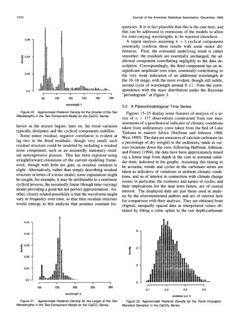wavelength 1 Figure 20. Approximate Posterior Density for the Smaller of the Two Wavelengths in the Two-Component Model for the CaCO3 Series. 3.2 A Paleoclimatological Time Series Figures 15-25 display some features of analysis of a series of n = 177 observations constructed from raw measurements of a geochemical indicator of climatic conditions taken from sedimentary cores taken from the bed of Lake Turkana in eastern Africa (Halfman and Johnson 1988; West 1995). The data are measures of calcium carbonate (as a percentage of dry weight) in the sediments, made at various locations down the core; following Halfman, Johnson, and Finney (1994), the data have been approximately timed via a linear map from depth in the core to nominal calendar time, indicated in the graphs. Assuming this timing to be accurate, trends and cycles in the carbonate series are havior as the seizure begins; later on, the trend variation typically dissipates and the cyclical components stabilize. Some minor residual, negative correlation is evident at lag two in the fitted residuals; though very small, such residual structure could be modeled by including a residual noise component, such as an assumedly stationary residual autoregressive process. This has been explored using straightforward extensions of the current modeling framework, though with little net gain, as residual variation is slight. Alternatively, rather than simply describing residual taken as indicative of variations in ambient climatic condistructure in terms of a noise model, some explanation might tions, and so of interest in connection with climate change be sought; for example, it may be attributable to a nonlinear issues; in particular, the existence and nature of cycles, and cyclical process, the assumedly linear (though time-varying) their implications for the near term future, are of central model providing a good but not perfect approximation. An- interest. The displayed data are just those used in analyother, closely related possibility is that the waveforms might sis by the aforementioned authors and are of interest here vary in frequency over time, so that then residual structure for comparison with their analysis. They are obtained from would emerge in this analysis that assumes constant freoriginal, unequally spaced data as interpolated values obtained by fitting a cubic spline to the raw depth:carbonate 0.05 0.04- 6- t0.03- 4 0.02- 2- 0.01 I0 150 200 250 300 100 150 200 250 300 wavelength 2 Figure 21. Approximate Posterior Density for the Larger of the Two Wavelengths in the Two-Component Model for the CaCO3 Series. 010.2 0.3 0.4 evolution s.d. 0 Fiue22. Approximate Posterior Density for the Trend Innovation Standard Deviation in the CaCO3 Series.
West: Inference on Cycles in Time Series 1311 60 20 40- 20- ~o10 5 s l] I Illalllilllli II I 0.0 0.05 0.10 0.15 evolution s.d. 1 Figure 23. Approximate Posterior Density for the Component Innovation Standard Deviation v/iw in the CaCO3 Series. 0.0 0.02 0.04 0.06 0.08 0.10 0.12 0.14 evolution s.d. 2 Figure 24. Approximate Posterior Density for the Component Innovation Standard Deviation Vw-2 in the CaCO3 Series. data, and then evaluating the interpolant at equally spaced expected; this may be viewed as tending to overfit the data points down the core prior to mapping to nominal real time. (partly supported by the observed though minor degree of The graphs display summary inferences, in a format anal- negative residual correlation). More informed priors on the ogous to that of the EEG analysis, for a two-component variance components to control to smaller values and hence model with a locally linear trend. As with the EEG analysis, smooth out some of the irregularity might be desirablewe use diffuse uniform priors for the square roots of vari- indeed, common practice with DLM's is to directly conance components. To summarize the outputs, there is some trol evolution variances to smaller values, perhaps through evidence of one subtle subcycle of wavelength in the 140- the use of discount factors (Pole, West, and Harrison 1994; 160-year range, and this echoes results of related data in West and Harrison 1989). this field (Halfman et al. 1994). Additional cyclical struc- The formulation in DLM terms permits application in ture, if present, lies in the 100-115-year range, with some contexts where the time series is irregularly spaced over suggestion of 80-100 years too; however, the estimated amtime or subject to missing values. Missing observations plitude of such secondary features is essentially negligible, are these data being as well described by a one-cycle model as directly subsumed by the usual sequential DLM analby a two-cycle model. And then the period of 150? is eviysis; prior to posterior update is vacuous if no data are denced only very weakly, the observation noise dominating observed. This leads neatly into the treatment of irreguthe data variation. larly spaced data, as developed by West and Harrison (1989, This example contrasts with the EEG analysis in that the chap. 10). Unequally spaced data can usually be treated by estimated trajectories of cyclical components are rather stable over time. In this sense it is apparenthat the models and approach essentially encompass the more usual context of harmonic regression with fixed sinusoids (Bretthorst 1988) 4 - in cases of low levels of evolution variance in the model components. Further and more penetrating analyses of these and re- 3 - lated data has been provided by West (1995). 4. CONCLUSIONS Some immediate issues arising in applications have to do with simulation sample sizes and convergence checks, standard considerations in Bayesian analyses via simulation, and, particularly, the choices of prior distributions for DLM variance components. The priors used in the foregoing examples are proper uniform distributions for v and each of the w3, with ranges that turn out not to conflict with the likelihood function. But as a result, as is clear from the figures, the underlying trend component of the model is inferred to be possibly rather more variable than perhaps 2 - 0 1.2 1.3 1.4 1.5 1.6 1.7 observation s.d. Figure 25. Approximate Posterior Density for the Observation Error Standard Deviation fv in the CaCO3 Series.
Page 1 and 2: Bayesian Inference in Cyclical Comp
Page 3 and 4: West: Inference on Cycles in Time S
Page 9: West: Inference on Cycles in Time S

Bayesian Inference in Cyclical Component Dynamic Linear Models

You also want an ePaper? Increase the reach of your titles

Delete template?

Save as template?