Bayesian Inference in Cyclical Component Dynamic Linear Models
Bayesian Inference in Cyclical Component Dynamic Linear Models
Bayesian Inference in Cyclical Component Dynamic Linear Models

You also want an ePaper? Increase the reach of your titles
YUMPU automatically turns print PDFs into web optimized ePapers that Google loves.
1302 Journal of the American Statistical Association, December 1995<br />
45 -<br />
sov<br />
40-<br />
.50<br />
100<br />
.150<br />
35 -<br />
30 -<br />
25-<br />
20-<br />
-200<br />
0 20 40 60 80 100<br />
time<br />
Figure 1. 1 10 Observations on an EEG Trace.<br />
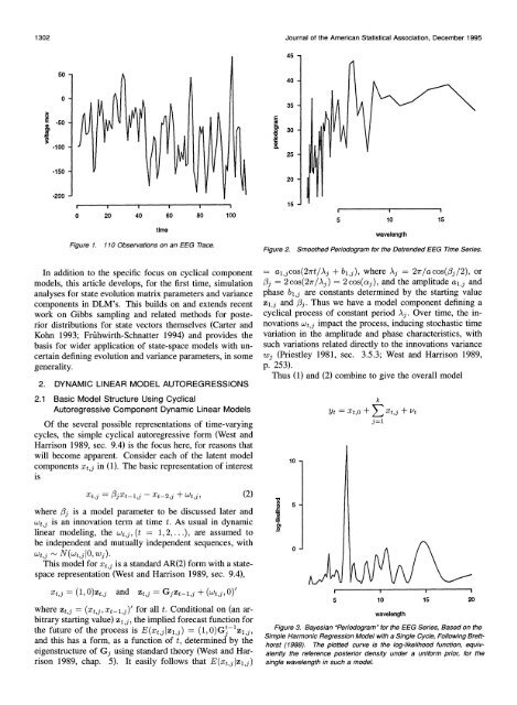
Figure 2.<br />
5 10 15<br />
wavelength<br />
Smoothed Periodogram for the Detrended EEG Time Series.<br />
In addition to the specific focus on cyclical component<br />
models, this article develops, for the first time, simulation<br />
analyses for state evolution matrix parameters and variance<br />
components <strong>in</strong> DLM's. This builds on and extends recent<br />
work on Gibbs sampl<strong>in</strong>g and related methods for posterior<br />
distributions for state vectors themselves (Carter and<br />
Kohn 1993; Fruhwirth-Schnatter 1994) and provides the<br />
basis for wider application of state-space models with uncerta<strong>in</strong><br />
def<strong>in</strong><strong>in</strong>g evolution and variance parameters, <strong>in</strong> some<br />
generality.<br />
2. DYNAMIC LINEAR MODEL AUTOREGRESSIONS<br />
2.1 Basic Model Structure Us<strong>in</strong>g <strong>Cyclical</strong><br />
Autoregressive <strong>Component</strong> <strong>Dynamic</strong> L<strong>in</strong>ear <strong>Models</strong><br />
Of the several possible representations of time-vary<strong>in</strong>g<br />
cycles, the simple cyclical autoregressive form (West and<br />
Harrison 1989, sec. 9.4) is the focus here, for reasons that<br />
will become apparent. Consider each of the latent model<br />
components xt,j <strong>in</strong> (1). The basic representation of <strong>in</strong>terest<br />
is<br />
= a,jcos(27rt/Aj + b,ij), where Aj = 27r/acos(C3/2), or<br />
Ij = 2cos(27r/Aj) = 2cos(aj), and the amplitude al,j and<br />
phase bl,j are constants determ<strong>in</strong>ed by the start<strong>in</strong>g value<br />
zij, and /3j. Thus we have a model component def<strong>in</strong><strong>in</strong>g a<br />
cyclical process of constant period Aj. Over time, the <strong>in</strong>novations<br />
w,j impact the process, <strong>in</strong>duc<strong>in</strong>g stochastic time<br />
variation <strong>in</strong> the amplitude and phase characteristics, with<br />
such variations related directly to the <strong>in</strong>novations variance<br />
wj (Priestley 1981, sec. 3.5.3; West and Harrison 1989,<br />
p. 253).<br />
Thus (1) and (2) comb<strong>in</strong>e to give the overall model<br />
10 -<br />
Yt =Xt,0 + E xt,j + vt<br />
j=1<br />
k<br />
Xtj = jXt1 -,j - Xt-2,j + Wtj (2)<br />
where /j is a model parameter to be discussed later and<br />
w,j is an <strong>in</strong>novation term at time t. As usual <strong>in</strong> dynamic<br />
l<strong>in</strong>ear model<strong>in</strong>g, the w,j, (t = 1, 2, .. .), are assumed to<br />
be <strong>in</strong>dependent and mutually <strong>in</strong>dependent sequences, with<br />
Wt,j -N(tj w IO, jw).<br />
This model for xt,j is a standard AR(2) form with a statespace<br />
representation (West and Harrison 1989, sec. 9.4),<br />
Xt,j = (1, O)zt,j and Zt, = Gjztl,3 + (t,j, 0)'<br />
where Zt, = (xt,j, Xti,j)' for all t. Conditional on (an arbitrary<br />
start<strong>in</strong>g value) z1,j, the implied forecast function for<br />
the future of the process is E(x+,;Iz,i) = (l,O)Gt-1z, ,<br />
and this has a form, as a function of t, determ<strong>in</strong>ed by the<br />
eigenstructure of Gj us<strong>in</strong>g standard theory (West and Harrison<br />
1989, chap. 5). It easily follows that E(xt,j|Zi,;)<br />
8 s<br />
0)<br />
0J<br />
0<br />
5 10 15 20<br />
wavelength<br />
Figure 3. <strong>Bayesian</strong> "Periodogram" for the EEG Series, Based on the<br />
Simple Harmonic Regression Model with a S<strong>in</strong>gle Cycle, Follow<strong>in</strong>g Bretthorst<br />
(1988). The plotted curve is the log-likelihood function, equivalently<br />
the reference posterior density under a uniform prior, for the<br />
s<strong>in</strong>gle wavelength <strong>in</strong> such a model.