Bayesian Inference in Cyclical Component Dynamic Linear Models

Bayesian Inference in Cyclical Component
Dynamic Linear Models
Mike WEST
Dynamic linear models (DLM's) with time-varying cyclical components are developed for the analysis of time series with persistent
though time-varying cyclical behavior. The development covers inference on wavelengths of possibly several persistent cycles in
nonstationary time series, permitting explicit time variation in amplitudes and phases of component waveforms, decomposition of
stochastic inputs into purely observational noise and innovations that impact on the waveform characteristics, with extensions to
incorporate ranges of (time-varying) time series and regression terms wihin the standard DLM context. Bayesian inference via
iterative stochastic simulation methods is developed and illustrated. Some indications of model extensions and generalizations are
given. In addition to the specific focus on cyclical component models, the development provides the basis for Bayesian inference,
via stochastic simulation, for state evolution matrix parameters and variance components in DLM's, building on recent work on
Gibbs sampling for state vectors in such models by other authors.
KEY WORDS: Autoregressive component dynamic linear model; Cyclical time series; Dynamic linear model; Markov chain
Monte Carlo.
1. INTRODUCTION
Applications of traditional dynamic linear models
(DLM's), or state-space models, with cyclical components
have to date been broadly restricted to contexts in which
periods of cyclical components are known and integer, the
typical contexts of seasonal modeling and time-varying harmonic
analysis (West and Harrison 1989, chap. 8). Problems
of inference about uncertain wavelengths of timevarying
cyclical components in such models have been untouched,
in part due to analytic complications. This article
begins to address such problems.
Consider a real-valued, zero-mean time series Yt observed
at times t = 1, 2, ... We deal with models of the form
k
Yt =Xt,0 + E Xt,j + vt, 1
j=1
where the k distinct, latent processes Xt,j, t - 1, 2,...,
represent persistent periodic components of distinct frequencies
and with, quite generally, possibly time-varying
amplitude and phase characteristics. The component xt,0
represents additional time series structure, including possibly
nonstationary trend or growth and regression effects,
and vt represents observation noise, typically combining
measurement, sampling, and residual misspecification errors.
Our interest lies specifically in models in which each
of the cyclical processes has the form xt,j = rjtcos(atjt
+ qjt), a sinusoid of fixed period Aj = 27r/aj, and stochastically
time-varying amplitude ajt and phase bjt. We are interested
in inference for the entire model to identify acyclic
trends and, simultaneously, the wavelengths Aj and the patterns
of behavior of the cyclical subseries xt,j over the period
of the observed data. One applied focus for such models
is in evaluating trends in the presence of periodicities of
uncertain wavelengths; another, more usual context is when
interest lies in identifying persistent subcycles, possibly of
generally low amplitude, in noisy series. The latter problem
is typified by climatological studies in which the existence
of subtle periodic components may influence discussions of
global climate change (see, for example, West 1995).
A complete model specification requires descriptions of
the precise forms of time-variation anticipated in amplitudes
and phases, and that is done here through the use of
cyclical form DLM's (West and Harrison 1989, chap. 8
and sec. 9.4). These models provide generalizations and
alternatives to more traditional parametric models, such as
harmonic regression (Bretthorst 1988) and stationary models,
with features common to all state-space models. In
particular, the key issue of time variation in cyclical components
naturally extends traditional harmonic regression
models. DLM's explicitly partition of sources of variation
into purely observation noise versus noise components affecting
signals, cyclical or otherwise. Thus the signals xt,j
have characteristics that change over time, to a greater or
lesser extent, and these changes are determined by noise
terms identified and distinct from the noise terms vt that affect
only the observations. In some problems, measurement
and sampling errors and possible additive outliers account
for a major component of observed data variation, and so
this explicit representation, which is absent from traditional
stationary time series models, is critical. Potential future
extensions to model outliers and abrupt changes in signal
form can build on existing modeling and intervention ideas
in DLM's (West and Harrison, chaps. 10 and 11). Further,
DLM representations allow for routine handling of missing
values and irregularly spaced data in time series (West
and Harrison, sec. 10.5), in contrast to standard stationary
time series and spectral methods. Moreover, the models include
traditional harmonic regressions (Bretthorst 1988) as
special cases, and so provide for the assessment of stable
cyclical forms within the more general dynamic framework,
and computational tools to fit essentially constant harmonic
components.
Mike West is Professor and Director, Institute of Statistics and Decision
Sciences, Duke University, Durham, NC 27708-0251. Partial support for
this work was provided by National Science Foundation Grants DMS-
9024792 and DMS-9311071.
1301
? 1995 American Statistical Association
Journal of the American Statistical Association
December 1995, Vol. 90, No. 432, Theory and Methods

1302 Journal of the American Statistical Association, December 1995
45 -
sov
40-
.50
100
.150
35 -
30 -
25-
20-
-200
0 20 40 60 80 100
time
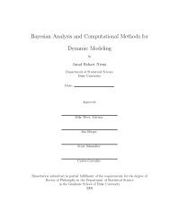
Figure 1. 1 10 Observations on an EEG Trace.
Figure 2.
5 10 15
wavelength
Smoothed Periodogram for the Detrended EEG Time Series.
In addition to the specific focus on cyclical component
models, this article develops, for the first time, simulation
analyses for state evolution matrix parameters and variance
components in DLM's. This builds on and extends recent
work on Gibbs sampling and related methods for posterior
distributions for state vectors themselves (Carter and
Kohn 1993; Fruhwirth-Schnatter 1994) and provides the
basis for wider application of state-space models with uncertain
defining evolution and variance parameters, in some
generality.
2. DYNAMIC LINEAR MODEL AUTOREGRESSIONS
2.1 Basic Model Structure Using Cyclical
Autoregressive Component Dynamic Linear Models
Of the several possible representations of time-varying
cycles, the simple cyclical autoregressive form (West and
Harrison 1989, sec. 9.4) is the focus here, for reasons that
will become apparent. Consider each of the latent model
components xt,j in (1). The basic representation of interest
is
= a,jcos(27rt/Aj + b,ij), where Aj = 27r/acos(C3/2), or
Ij = 2cos(27r/Aj) = 2cos(aj), and the amplitude al,j and
phase bl,j are constants determined by the starting value
zij, and /3j. Thus we have a model component defining a
cyclical process of constant period Aj. Over time, the innovations
w,j impact the process, inducing stochastic time
variation in the amplitude and phase characteristics, with
such variations related directly to the innovations variance
wj (Priestley 1981, sec. 3.5.3; West and Harrison 1989,
p. 253).
Thus (1) and (2) combine to give the overall model
10 -
Yt =Xt,0 + E xt,j + vt
j=1
k
Xtj = jXt1 -,j - Xt-2,j + Wtj (2)
where /j is a model parameter to be discussed later and
w,j is an innovation term at time t. As usual in dynamic
linear modeling, the w,j, (t = 1, 2, .. .), are assumed to
be independent and mutually independent sequences, with
Wt,j -N(tj w IO, jw).
This model for xt,j is a standard AR(2) form with a statespace
representation (West and Harrison 1989, sec. 9.4),
Xt,j = (1, O)zt,j and Zt, = Gjztl,3 + (t,j, 0)'
where Zt, = (xt,j, Xti,j)' for all t. Conditional on (an arbitrary
starting value) z1,j, the implied forecast function for
the future of the process is E(x+,;Iz,i) = (l,O)Gt-1z, ,
and this has a form, as a function of t, determined by the
eigenstructure of Gj using standard theory (West and Harrison
1989, chap. 5). It easily follows that E(xt,j|Zi,;)
8 s
0)
0J
0
5 10 15 20
wavelength
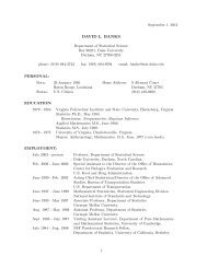
Figure 3. Bayesian "Periodogram" for the EEG Series, Based on the
Simple Harmonic Regression Model with a Single Cycle, Following Bretthorst
(1988). The plotted curve is the log-likelihood function, equivalently
the reference posterior density under a uniform prior, for the
single wavelength in such a model.

West: Inference on Cycles in Time Series 1303
and
Xt,; =3jXt-1,j -Xt-2,j + Wtj (j 1, , k), (3)
100 -
so - ++ +
with /3 = 2 cos(27r/Aj) for j = ,... , k. In addition to
the earlier assumptions about the innovations process, it
is further assumed that the observational errors form an
independent sequence and are independent of the Wt,j, with
Vt N(vtIO,v).
It remains to model the acyclic trend process xt,0. To
take a simple and specific model, though one of much utility
and used in an illustration that follows, we suppose here
a first-order polynomial. Other DLM forms are possible,
of course, but the first-order model provides for simple but
flexible local smoothing of underlying, acyclical, and nonstationary
trends in the absence of more informed trend
models such as regression DLM's. Then (following West
and Harrison 1989, chap. 2),
Xt,O = Xt-1,0 + W'tO,
where wt,O N(w)t,o 0, wo) independently over time and independently
of the innovations wtj in (3). This trend model
combines with (3) to give the general DLM representation
and
Yt = F'zt + Vt
with the following ingredients:
Zt = Gzt_l + 6t, (4)
Xt,O 1
Xt,1
Xt,21
Zt= St12 F= 0
Xt,k 1
Xt-l,k 0
/1
:1 -1
1 0
/32 1
G= 1 0
50 + + +
-200 + + ++
l
40 o 2
6
>0 ~~~~~~ +
Lmt +
+~~~ 4k
Here - is+ b so t +
-200 ~ ~ ~ ~ + + +
0 20 40 60 80 100
-100
vaiac mari W igw;w ;W,0 N . ***
)
time
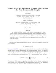
Figure 4. Estimated Acyctlc Trend, With One Standard Deviation
Limits, for the EEG Series.
Here G is block-diagonal, so the "empty" entries in (5)
are all zero. Note further that 6t -N (6t 0O, W) with diagonal
variance matrix W = diag(wo; wl, 0; W2, o; ... ; Wk, 0).
2.2 Posterior Structure and Framework of Simulation
Analysis
Assume the model (4) for the series of n observations
{Yt; t = 1, ... , n}. Inference is required on the wavelengths
A, equivalently the state parameters 3 = {i3,- ... , !k },
the variance components v and W, the individual "latent"
stochastic subcycles Xj d {xt,j; t = O.... ,n} for each
j = 1,...,k, and the trend component Xo df {Xt,o; t
= O,... ,}. In standard notation, define Dt = {yt, Dt-i}
for the information set available at time t, having observed
the time series value at that time; at t = 0, Do represents
all initial information including the model specification and
assumptions. Assume the analysis to be closed to external
inputs and interventions, so that Dt is a sufficient summary
of the history at time t. Hence analysis involves specifying
100
50 -
0
4
Wt ,O
Wt, 1
0
wt,2
nt ,k
/3k -1
1 0
t= 0' 5
0
-50
-150 -'
-200 -
., , , , I
0 20 40 60 80 100
time
Figure 5. Fitted Values for the EEG Series.

1304 Journal of the American Statistical Association, December 1995
(0
150
100
50
-50-
-100 -
-150 -
r I I
0 20 40 60 80 100
time
Figure 6. Estimated Residuals From the EEG Data Analysis.
classes of priors for {/3, v, W, zo}, then computing posterior
distributions and appropriate summaries for {/3, v, W, Z},
where Z is the complete set of state variables,
def
Analyses here are based on priors of the form
p(A, v, W, zo) = p(O)p(V)p(zo)
k
fi p(Wj),
j=O
where p(.) is generic notation for density function. Extensions
to incorporate further prior dependencies are possible.
On this basis, the following structure may be deduced:
1. Assume that /, v, and W are specified. Then (4) is
a standard normal DLM whose analysis is fully defined in
closed analytic form (West and Harrison 1989, chap. 4) if
it is assumed that the prior for the initial state vector zo is
a specified normal distribution, zo N(zo I0m, CO). Note
that this prior may depend on the conditioning values of
/, v, and W, though this is of little practical relevance, and
so no such dependence is assumed throughout. Standard
updating results (West and Harrison 1989, sec. 4.3) apply to
sequentially compute moments mt and Ct of the posterior
normal distributions for (ztlDt) at all times t. Because the
values of /, v, and W are conditioned on, make this explicit
in the notation; thus it is simple to compute the moments
defining the "on-line" posteriors,
(zt Dt, /, v, W) - N(ztImt, Ct), (t = 1, ... , n). (6)
2. Assume the complete set of subseries Z = {Xo,
X1, . .., Xk} to be specified in addition to /, and focus on
inference about the variance components v and W. Under
the assumed conditionally independent prior,
with the following components:
(a) p(vID7, Z) oC p(v)v-n/2exp(-s/(2v)), where s
- i=i(ytt-F'zt)2;
(b) p(woIXo) CX p(wo)w-n/2exp(-ro/(2wo)), where
ro = Z -i(xt,O-xt_1,0)2; and
(c) for each j = 1,.. ,k, p(wj lof, Xj) oc p(wj)wf(n 1)/2
x exp(-rj/(2wj)), and with sum of squares rj
Zt=2(xt,j - /jXtl,j + Xt2,J).
It is evident that independent inverse gamma priors for
all k + 2 scalar variance components here are conditionally
conjugate, the sets of posteriors described then being inverse
gamma forms with updated shape and scale parameters
in each case. Other priors may be used. One recommended
alternative is rather uninformative priors in which
the standard deviations ar and wj for each j are assumed
to be uniformly distributed over finite and specified
ranges. Then the foregoing conditional posteriors are truncated
gamma distributions.
3. Assume the complete set of subseries Z = {Xo,
Xl, . ..., Xk } to be specified in addition to the variance components
v and W, and focus on inference about 3. For each
j 1, ..., k, define scalar quantities bj and Bj by
B7 I=
Then
n
n
X2
1j and bj = Bj Z(xt,J + xt2,J)xt1,J
t=2 t=2
p(lDn7,v,W,Z) p(f3W, Z)
k
O? p(f) 11 exp(-(j -bj)2/(2Bjwj))
j=1
It is now easy to see that simulation-based analysis using
Markov chain Monte Carlo is straightforward to implement.
Iterative sampling of conditional posterior distributions de-
150 l
100 -
50-
-50-
-100 -
-150
0 20 40 60 80 100
(8)
k
= p(v |Dn:Z)p(wo ]Xo )flp(wj l/3i,Xj ), (7)
j=1
time
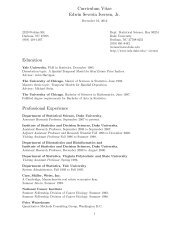
Figure 7. Estimated Trajectory Over Time, With Uncertainty Bands,
for the First Cyclical Component of a Two-Cycle Model for the EEG
Series.

West: Inference on Cycles in Time Series 1305
150 -
100
50~~~~~~~~~~~~~~~~~~~~~~~~~~~~~
-
50
-50 -
-100
-150
This produces a sequence ZnZn- . ....I ZO, equivalently the
set Z, as required. The computations are quite straightforward
when it is recognized that on the basis of the strong
conditional independence structure in the model (4),
p(zt IDn , OiV- W, Zt+1 I Zt+2, I ,.
Zn)
-- p(ztlDn, ,B, vI WI Zt+1).
Furthermore, combining the second equation in (4) with
the on-line posterior in (6) leads to
p(ztJDn,/ ,Vt, WI Zt+l) x N(ztlmt, Ct)N(zt+I IGzt, W),
0 20 40 60 80 100
time
Figure 8. Estimated Trajectory Over Time, With Uncertainty Bands,
for the Second Cyclical Component of a Two-Cycle Model for the EEG
Series.
fined earlier may proceed by sampling through the sequence
*>p(ZIDni/,B,V,W)
k
> p(v Dn,Z)p(wo X0) flp(Wj li0Xj )
j=1
---- > pP IW , Z) ---- > ... (9)
at each iteration.
The second stage here requires little further comment;
the conditional posteriors for all variance components are
outlined under Step 2. Steps 1 and 3 are considered in more
detail in the next two sections. Before proceeding, note that
(as in Carter and Kohn 1994 and Friihwirth-Schnatter 1994),
successive draws under this simulation scheme will eventually
resemble draws from the full joint posterior distribution
for {B3, v, W, Z}. The very general results provided by
Smith and Roberts (1993, thm. 1 and lem. 1 of appendix),
for example, are applicable.
2.3 Simulation of Model Component Subseries
The first stage of each simulation iteration (9) involves
sampling the conditional posterior of the full set Z of subseries,
p(Z IDn, 3, v, W). Recent work by Carter and Kohn
(1993) and Fruhwirth-Schnatter (1994) provides the basis
for this step; earlier ideas appear in work of Carlin, Polson,
and Stoffer (1992), though the specific algorithms of the
first two references are more appropriate, as was made explicit
by Carter and Kohn. A value of Z = {zo, . . ., Zn } may
be drawn from the rather complicated and high-dimensional
full posterior p(Z Dt, 13, v, W) as follows:
* Simulate a value of Zn from (ZnlDn,/ y3 v, W)
N (Zn Imn, Cn), simply (6) at t - n.
* For each t = n - I,n - 2, .0. I, O reducing
the time index by one at each step, simulate
a value of Zt from the conditional posterior
p(zt Dr,, 43, V, W, zt+, Zt+2 ... ,: Zn); at each stage the
conditioning values of znr,zn-,... here are those
just generated.
(10)
so that p(zt IDn, ,3, v, W, Zt+1) is normal with moments easily
found; in detail, the mean and variance matrix are
mt + At(zt+l - Gmt) and Ct - AtQtA', where Qt
GCtG' + W and At = CtGQT1. This normal distribution
is easily sampled, and then sequencing down
through t n- ,n - 2,...,0 produces a full draw,
Z { Zn ZO} as required. Further details have been
given by Carter and Kohn (1994) and Fruhwirth-Schnatter
(1994).
A slight modification of the foregoing development that
produces a more easily implemented algorithm involves
simulating Z by drawing each of the model component subseries
sequentially conditional on values of the other sub-
series. Specifically, for each j 0, . . . k, introduce Z()
= Z\Xj, the set Z with Xj= {xj,o,...,x3,n} removed;
write J for the corresponding index set J = {O,...,j
- 1, j + 1, ..., k}. Fix the index j and suppose that
Z() is set at the previously sampled values. Compute the
adjusted time series values Yt,j = Yt - >hCJ
Xt,h, and write
Zt,; = (Xt,j, Xt- ,j) for all t. Then, based on a previously
simulated full set of subseries Z, a new set is generated by
the following procedure:
4 -
3 -
2 -
o J
.M1ti,g ...
5.5 6.0 6.5 7.0
wavelength 1
Figure 9. Approximate Posterior Density for the Smaller of the Two
Wavelengths in the Two-Component Model for the EEG Series.

1306 Journal of the American Statistical Association, December 1995
Now the foregoing development in terms of the full
0.4
state vector zt can be reworked in terms of the twodimensional
vectors zt,j. Routine DLM updating is trivially
performed to provide the collection of "on-line" poste-
0.3
riors (zt,jjDt, Z U3, v, W) N(zt,jImt,j, Ct,j), whence
trivial calculations lead to (zt,jID, ZU)A , v, W, Zt+l,j)
using the theory as in (9); this produces the normal
0.2-
with moments mt,j + At,j(zt+i,j - Gjmt,j) and Ct,
-Atj, Qt,j At , where Qt,j = Gj Ct,j G + Wj and At,
= Ct,j Gj Q- 1. Here
0.1
Gj 1=(3 i0) and
I, I1
Wj =(j 0)
I1 Il lll i Itl .. I I
0.0 dI IIIIIIIIhh
The original algorithm that samples each complete vector
8 10 12 14 16 18 20 zt at each iteration theoretically converges faster; breaking
zt
wavelength 2
into constituents and sampling these conditionally as in
the second algorithm theoretically slows convergence by in-
Figure 10. Approximate Posterior Density for the Larger of the Two ducing higher correlations between successive draws. But
Wavelengths in the Two-Component Model for the EEG Series. the latter algorithm is very much faster in models with even
very moderate values of k; the matrix inversions Q71 re-
1. Set j = 0.
quired at each t in the former algorithm lead to significant
2. Fix Z() at the most recently sampled values, and com- overheads. Some approximations to avoid repeat matrix
pute the adjusted series {Yt,j}.
inversions are possible, though their effectiveness is unex-
3. Noting that conditional on Zi), the adjusted time se- plored. Experience with both algorithms has suggested that
ries follows a DLM with state vectors xt,j, the routine just the faster, conditional approach is in fact typically adequate
outlined (following Carter and Kohn 1994 and Fruhwirth- in terms of producing simulations in close agreement with
Schnatter 1994) applies to simulate the full set Xj from the former algorithm; further investigations are needed to
(XjJ Dn, Z zU) 3, v, xW zt+?1,3); perform this simulation to compare and assess the two approaches for both statistical
obtain a new value X .
and computational efficiencies.
4. If j < k, then update j to j + 1, go to Step 1 and
continue.
2.4 Simulation of Wavelengths
At Step 3 here the computations are trivial. In case j = 0, Restricting wavelengths to Aj > 2, the Nyquist limit
so that Xo is the locally constant trend subseries, and practical limit for identification of cycles, the map between
Aj > 2 and 3j is monotonically decreasing, with 3j
Yt,o = Xt,O + Vt
= 2 cos(2ir/Aj) lying between +2 (indeed, rather often, relevant
wavelengths will exceed 4, so that
and
3j > 0.) Hence we
can work interchangeably with either the wavelengths or the
Xt,O = Xt- 1,0 + Wt,O
0.06 -
DLM updating is now trivial, producing (xt,o Dt IZ(O)
3, v, W) -
N(xt,oJmt,o, Ct,o) for all t. Then, as ear- 0.05
lier, (xt,oJDn,Z(?),3,v,V, xt+1iO) is normal with moments
mt,o + At,o(xt+?,o - mt,o) and Ct,o - A 2 o(Ct o
0.04-
+wo), where At,o = Ct,O/(Ct,O + wo). So the subseries
Xo is simply generated by sampling xn,O from
the final 0.03-
posterior N(xn,oJMn,O, CT,O), then sequencing
down through t = n - 1, n - 2,... , 0, sampling from
(Xt,OJDn,Z(0)1)3,v,W,xt+?io) and substituting the latest 0.02-
draw of xt+,,o in conditioning at each step.
In the case of any one of the cyclical subseries j
0.01
= 1, ... , k, the conditional DLM is
Yt,j = (1,0)zt,j+ Vt
10 20 30 40
and
evolution s.d. 0
Ztj= (pi; ~o1 )Ztil,3 ? (wti ) - Figure 11. Approximate Posterior Density for the Trend Innovation
Standard Deviation +/i in the EEG Analysis.

West: Inference on Cycles in Time Series 1307
0.15 -
0.10 -
0.15
0.05
0.0 1 .
0 10 20 30
evolution s.d. 1
Figure 12. Approximate Posterior Density for the Component Innovation
Standard Deviation f/w- in the EEG Analysis.
0.0 _
0 5 10 15 20
evolution s.d. 2
Figure 13. Approximate Posterior Density for the Component Innovation
Standard Deviation vw2 in the EEG Analysis.
autoregressive coefficients; simulation of the 3 parameters (8) implies
from conditional posteriors p(,3W, Z) in (9) produces sampled
wavelengths via the identities Aj = 27r/arccos(ij/2) p(/j3IDn, :(i), v, W, Z) cX N(,3j bj, Bjwj),
for each j, and posterior inferences may be explored di-
(d( 1 i j+)l
rectly from the samples. Conversely, it is natural to think
in terms of priors for the wavelengths and then transform So sampling may proceed conditionally, cycling through
to deduce priors for the da.
the /j parameters given previously sampled values of 3(i)
(among other things), with new values of the
Strict constraints on wavelengths may be enforced
Oj trivially
generated from a truncated normals.
through the prior distribution. Some form of constraint
As noted, other priors might be used, as context deis
necessary for identification-note that the model remands,
based on transforming from plausible priors for
mains the same under arbitrary permutation of the wave- the A3. Working in terms of conditional priors is natural,
length indices. The constraint here is simply the ordering and the foregoing development is modified only through
A1 < A2 < ... < Ak under the prior, and this provides conditionals p(j[3U(i)) that will be other than uniforms.
parameter identification. Other strict constraints, such as The conditional posteriors are then p(j3 IDn, d3(i), v, W, Z)
enforcing a minimum separation between any two wave- c< p(Oj3 M(i))N(3jjbj,Bjwj) so the analysis differs only
lengths, may be desirable in some applications and can be technically; sampling these conditional posteriors will gensimilarly
introduced.
In an illustration that follows we use conditional priors
that are effectively reference priors for the Oj conditional
on all other parameters, simply conditional uni- 0.08-
forms. This provides a benchmark analysis. Alternative
analyses based on plausible, informed priors for the Aj
0.06-
that induce specific forms of priors for the Oj parameters
may be similarly implemented within this framework.
Write U(. la, b) for the uniform distribution on (a, b) and
0.04
suppose a specified minimum wavelength separation of
6 > 0 time units (e.g., 6 = 1). The class of priors used
is defined by the set of complete conditionals (lujj(i)), 0.02 -
where :3() = \ ij _ { ,3. ..,/3j-1,/3j+1, . . ,k}, for
all j. Extend notation to include fixed and specified lim-
its on wavelengths A0 < Ak+l; often Ao = 2 and Ak+1
is some appropriately large value. Then take conditionals
(p3ylp(J)) U(p3jl3p~ i34l,(2) for all j, where j)
=2 cos(2wr/(Aj_i + 6)) and p3(2)l = 2 cos(2w/(A3+1 - 6)).
Under the joint prior so specified, the conditional posterior
0.0
I I I I
20 30 40 50
observation s.d.
Figure 14. Approximate Posterior Density for the Observation Error
Standard Deviation fv in the EEG Analysis.

1308 Journal of the American Statistical Association, December 1995
12 +
10 +++;++
61+a 4~~~X + * + + ++ +
co - 8
+
+
+
+ 4+++ +
+ . 4
+
+ + 4? ++I.
+ + +~~~~~~~~
co ~~~~~~~~~~~~++
++~~~~~~~~~~
2
-500 0 500 1000
nominal years AD
Figure 15. 177 Observations on Calcium Carbonate Prevalence
(as Percent of Dry Weight) in an African Lake Sediment Core, Plotted
Against Nominal Calendar Years AD Imputed Following Halfman,
Johnson, and Showers (1994). The estimated acyclic trend, with one
standard deviation limits, for the series based on the DLM described in
Section 3 is superimposed.
erally be more complicated than in the case of truncated
normals, and rejection methods will be needed.
3.1 An EEG Time Series
3. ILLUSTRATIONS
Figures 1-14 display some features of analysis of a series
of nr= 110 electroencephalogram (EEG) recordings
from the scalp of an individual undergoing electroconvulsive
therapy (ECT). These data were provided by Dr Andrew
Krystal in Psychiatry at Duke University and arise in
studies of waveform characteristics in multichannel EEG
signal analyses; these studies are germane to assessments
of differing ECT protocols (see, for example, Krystal et al.
1992). Comparison of two or more such time series underlies
part of the study, and appropriate modeling of individual
time series represents a starting position for comparative
analyses. Here attention focuses on the single series
appearing in Figure 1 and the identification and estimation
of time-varying periodicities in the data (further substantive
developments of this study will be reported elsewhere). The
actual series shown is a short segment of a much longer series
from just one of several channels, and the numbers are
raw digitized values generated prior to conversion to electrical
potentials. There are nr= 110 observations over a
total time span of just over 1 second, corresponding to the
very start of an ECT-induced seizure.
Figure 1 plots the raw data over time; periodicities are evident,
as are variations in amplitude over time, and there are
noticeable nonlinear but apparently acyclic trends underlying
the evolution of the series. Some initial exploratory
graphics geared to identifying periodicities appear in Figures
2 and 3. These are based on a detrended series computed
by subtracting an estimate of an underlying trend
over time. (This estimated trend, from lowess in S-Plus,
is similar to that in the DLM analysis reported here, and
the details of how it was computed are not important here.)
Figure 2 shows the smoothed periodogram estimate of the
spectral density function (using the default spec.pgram in
S-Plus) for the detrended data and plotted as functions of
wavelength rather than frequency. Figure 3 displays the
likelihood/Bayesian analog, namely the (integrated) loglikelihood
function for wavelength A in a constant, singlecycle
harmonic regression model (see, for example, Bretthorst
1988, chap. 3); this represents the log-posterior under
a uniform prior for A. (Note that, as is theoretically the case
whatever the data, the log-likelihood here is bounded below,
so that a proper posterior distribution is obtained only
under a proper prior for A.) Qualitatively, these figures indicate
high power at wavelengths around A = 6, with some
possible contributions in the wavelength range 10-15. Note
that qualitatively similar conclusions are arrived at using
the raw data, rather than the specific detrended version used
here. The differences are that additional and apparently important
peaks arise in the periodogram and log-likelihood
functions at much higher wavelengths; these peaks are induced
by the underlying acyclic trends in the data rather
than real low-frequency periodicities.
On use of these exploratory graphical methods is to identify
suitable starting values for wavelengths in simulation
analysis of DLM autoregression, as described in Section 2.
Such was done in various analyses of these data; results
from a model with k = 2 component are summarized. This
analysis assumed priors as follows:
* Uninformative, independent priors for the initial level
of the series, x1,0, and the initial values of the component
subcycles, x1,j and xo,j for j = 1, 2; specifically,
N(xi,o10, 1,000) and N(zi 0,1,000I), where I is the
identity matrix.
* Conditionally uniform priors for the wavelength coefficients
3 induced by constraints on wavelengths of
2.0 < A. < 25.0, and a minimum separation of one
wavelength. A2 > A1 + 1.0 (though this turns out to
be nonbinding, as the likelihood function gives little
support to close values of the two wavelengths.)
12 -
J
12J
c~~,8 I~
1I I I I
-500 0 500 1000
nominal years AD
Figure 16. Fitted Values for the CaCO3 Series.

West: Inference on Cycles in Time Series 1309
6
6
4
4
2
e 0
-2
2
0
-2
-4
.4
-6
*500 0 500 1000
nominal years AD
Figure 17. Estimated Residuals From the CaCO3 Data Analysis.
-6
-500 0 500 1000
nominal years AD
Figure 18. Estimated Trajectory Over Time, With Uncertainty Bands,
for the First Cyclical Component of a Two-Cycle Model for the CaCO3
Series.
analyses that indicated some minor residual periodicities at
Proper priors for the variance components induced
by uniform priors for the corresponding standard deigher
wavelengths between 8 and 15; the posterior in frame
viations: p(v) oc v-l/2 over 0 < v < 104; simi-
1.10 has mass around A2 12 ? 3; note the high degree of
larly, for each of the evolution variances the prior is uncertainty. Figure 8 indicates that although the estimated
p(Wj) oc W1 1/2 over 0 < wj < 625. Other
amplitude is apparently substantial and important during
priors might
be used; these uniform (for standar deviations) priors the latter half of the observation period, uncertainty about
are assumed to provide a baseline or reference analy- this subcycle is relatively high throughouthe period. Be-
SiS.
cause of the increased contribution from this component in
the later stages, future predictions are affected, and so the
component is indeed quite relevant despite the high degree
of uncertainty. It was noted earlier that the data arose at the
very start of an ECT-induced seizure, and these summary
inferences are consistent with initial transient movement in
underlying trend plus initial variation in the cyclical be-
The priors here are proper and rather uninformative. The
simulation analysis ran through 10,000 iterations of the
Gibbs sampling scheme before any draws were saved; this
period of "burn-in" to convergence is quite conservative,
as repeat runs with differing starting values confirm. Following
this, 1 million iterations were run; the graphs here
display summaries of 10,000 of these samples obtained at
every 100th iteration. This substantially reduces correlations
between successive draws. All approximate posterior
inferences here are based directly on the Monte Carlo
draws, in terms of histograms of the 10,000 sampled values
for all parameters, simple sample means and standar deviations,
and so forth. Figure 4 provides a scatterplot of the
data over time with the estimated trajectory of the underlying
trend superimposed; the full line represents E(xt,o D,)
over t = 1, .. ., n, and the dashed lines provide uncertainties
in terms of ? V(xt,otDn). Similar trajectories for the
k = 2 subcycles appear in Figures 7 and 8, plotted with
the same range as the data. Figures 5 and 6 display the
fitted values and residuals. Figures 9-14 display posteriors
for the wavelengths and variance components. Figures
7 and 9 confirm the subcycle with a wavelength around
A1 6.3 ? .2. The former frame indicates the amplitude
over time of this component, apparently negligible during
the first 20 or 30 time intervals but quite prominent and persistent
later on. The relevance of a dynamic model allowing
for time variation in amplitudes is clear here. The second
component picks up on the periodogram-based exploratory
6
4-
2
0 A ~ ~~ A *-'
~~~~~~ S 1
0
-2
-4
-6
-500 0 500 1000
nominal years AD
Figure 19. Estimated Trajectory Over Time, With Uncertainty Bands,
for the Second Cyclical Component of a Two-Cycle Model for the CaCO3
Series.

1310 Journal of the American Statistical Association, December 1995
0.06
. 0.04 -
2
a)
0.02-
02 ,
I 1;Il;
i,iZXlllUIJII,,
I
80 100 120 140 160 180
I,.
quencies. It is in fact plausible that this is the case here, and
this can be addressed in extensions of the models to allow
for time-varying wavelengths, to be reported elsewhere.
A repeat analysis assuming k = 3 cyclical components
essentially confirms these results with some minor differences.
First, the estimated underlying trend is rather
smoother; the residuals are essentially unchanged, the additional
component contributing negligibly to the data description.
Correspondingly, the third component has an insignificant
amplitude over time, essentially contributing to
the very weak indication of an additional wavelength in
the 10-16 range, with the more evident, though still subtle,
second cycle of wavelength around 8-11. Note the correspondence
with the mass distribution under the Bayesian
"periodogram" in Figure 3.
wavelength 1
Figure 20. Approximate Posterior Density for the Smaller of the Two
Wavelengths in the Two-Component Model for the CaCO3 Series.
3.2 A Paleoclimatological Time Series
Figures 15-25 display some features of analysis of a series
of n = 177 observations constructed from raw measurements
of a geochemical indicator of climatic conditions
taken from sedimentary cores taken from the bed of Lake
Turkana in eastern Africa (Halfman and Johnson 1988;
West 1995). The data are measures of calcium carbonate (as
a percentage of dry weight) in the sediments, made at various
locations down the core; following Halfman, Johnson,
and Finney (1994), the data have been approximately timed
via a linear map from depth in the core to nominal calendar
time, indicated in the graphs. Assuming this timing to
be accurate, trends and cycles in the carbonate series are
havior as the seizure begins; later on, the trend variation
typically dissipates and the cyclical components stabilize.
Some minor residual, negative correlation is evident at
lag two in the fitted residuals; though very small, such
residual structure could be modeled by including a residual
noise component, such as an assumedly stationary residual
autoregressive process. This has been explored using
straightforward extensions of the current modeling framework,
though with little net gain, as residual variation is
slight. Alternatively, rather than simply describing residual taken as indicative of variations in ambient climatic condistructure
in terms of a noise model, some explanation might
tions, and so of interest in connection with climate change
be sought; for example, it may be attributable to a nonlinear
issues; in particular, the existence and nature of cycles, and
cyclical process, the assumedly linear (though time-varying) their implications for the near term future, are of central
model providing a good but not perfect approximation. An- interest. The displayed data are just those used in analyother,
closely related possibility is that the waveforms might sis by the aforementioned authors and are of interest here
vary in frequency over time, so that then residual structure for comparison with their analysis. They are obtained from
would emerge in this analysis that assumes constant freoriginal,
unequally spaced data as interpolated values obtained
by fitting a cubic spline to the raw depth:carbonate
0.05
0.04-
6-
t0.03-
4
0.02-
2-
0.01
I0 150 200 250 300
100 150 200 250 300
wavelength 2
Figure 21. Approximate Posterior Density for the Larger of the Two
Wavelengths in the Two-Component Model for the CaCO3 Series.
010.2 0.3 0.4
evolution s.d. 0
Fiue22. Approximate Posterior Density for the Trend Innovation
Standard Deviation in the CaCO3 Series.

West: Inference on Cycles in Time Series 1311
60
20
40-
20-
~o10
5 s l] I Illalllilllli
II I
0.0 0.05 0.10 0.15
evolution s.d. 1
Figure 23. Approximate Posterior Density for the Component Innovation
Standard Deviation v/iw in the CaCO3 Series.
0.0 0.02 0.04 0.06 0.08 0.10 0.12 0.14
evolution s.d. 2
Figure 24. Approximate Posterior Density for the Component Innovation
Standard Deviation Vw-2 in the CaCO3 Series.
data, and then evaluating the interpolant at equally spaced expected; this may be viewed as tending to overfit the data
points down the core prior to mapping to nominal real time. (partly supported by the observed though minor degree of
The graphs display summary inferences, in a format anal- negative residual correlation). More informed priors on the
ogous to that of the EEG analysis, for a two-component variance components to control to smaller values and hence
model with a locally linear trend. As with the EEG analysis, smooth out some of the irregularity might be desirablewe
use diffuse uniform priors for the square roots of vari- indeed, common practice with DLM's is to directly conance
components. To summarize the outputs, there is some trol evolution variances to smaller values, perhaps through
evidence of one subtle subcycle of wavelength in the 140- the use of discount factors (Pole, West, and Harrison 1994;
160-year range, and this echoes results of related data in
West and Harrison 1989).
this field (Halfman et al. 1994). Additional cyclical struc-
The formulation in DLM terms permits application in
ture, if present, lies in the 100-115-year range, with some
contexts where the time series is irregularly spaced over
suggestion of 80-100 years too; however, the estimated amtime
or subject to missing values. Missing observations
plitude of such secondary features is essentially negligible,
are
these data being as well described by a one-cycle model as
directly subsumed by the usual sequential DLM analby
a two-cycle model. And then the period of 150? is eviysis;
prior to posterior update is vacuous if no data are
denced only very weakly, the observation noise dominating
observed. This leads neatly into the treatment of irreguthe
data variation.
larly spaced data, as developed by West and Harrison (1989,
This example contrasts with the EEG analysis in that the chap. 10). Unequally spaced data can usually be treated by
estimated trajectories of cyclical components are rather stable
over time. In this sense it is apparenthat the models and
approach essentially encompass the more usual context of
harmonic regression with fixed sinusoids (Bretthorst 1988) 4 -
in cases of low levels of evolution variance in the model
components.
Further and more penetrating analyses of these and re-
3 -
lated data has been provided by West (1995).
4. CONCLUSIONS
Some immediate issues arising in applications have to
do with simulation sample sizes and convergence checks,
standard considerations in Bayesian analyses via simulation,
and, particularly, the choices of prior distributions for
DLM variance components. The priors used in the foregoing
examples are proper uniform distributions for v and
each of the w3, with ranges that turn out not to conflict with
the likelihood function. But as a result, as is clear from the
figures, the underlying trend component of the model is
inferred to be possibly rather more variable than perhaps
2 -
0
1.2 1.3 1.4 1.5 1.6 1.7
observation s.d.
Figure 25. Approximate Posterior Density for the Observation Error
Standard Deviation fv in the CaCO3 Series.

1312 Journal of the American Statistical Association, December 1995
identifying a base minimum time interval underlying the
observed times of observations and developing the equally
spaced DLM on that time scale. Then the times with no
observations are treated as points of missing data. This is
important for application. For example, these models are
currently in development as part of a broad study of the
geochemical indicators of climatic change used in the example,
in which raw data series are irregularly spaced (West
1995). Indeed, the timings of observations there are subject
to uncertainties that introduce additional complications that
can be accommodated with further modeling extensions of
obvious utility in other applications (West 1995, sec. 4).
The DLM formulation also permits access to other model
consequences, including predictive aspects. If relevant and
desired in an application, predictions may be routinely generated
from the simulation analysis. For each sampled set
of parameters and subcycles, insert the values into model
(4) and simply project into the future to produce a set of
sampled "futures" of the series. Averaging produces approximate
marginal predictive means and other features of
marginal forecast distributions. But though they are useful
(and traditional), marginal inferences represent crude summaries
of full joint predictive distributions, and other ways
of exploring and summarizing and sets of sequences of such
possible "futures" are needed. This represents an area open
to investigation.
The specific models here are clearly extensible to unrestricted
autoregressive components (Pole and West 1990;
West and Harrison 1989, sec. 9.4) to model stationary cyclical
behavior and additional residual time series structure in
the data, as mentioned in the EEG example. The simulation
framework directly extends to such models, as additive autoregressive
component simply introduce further uncertain
parameters into the system matrix G in (4). Such models
are currently under investigation in specific application contexts.
[Received January 1994. Revised March 1995.]
REFERENCES
Bretthorst, G. L. (1988), Bayesian Spectrum Analysis and Parameter Estimation,
New York: Springer-Verlag.
Carlin, B. P., Polson, N. G., and Stoffer, D. S. (1992), "A Monte Carlo
Approach to Nonnormal and Nonlinear State-Space Modeling," Journal
of the American Statistical Association, 87, 493-500.
Carter, C. K., and Kohn, R. (1994), "On Gibbs Sampling for State-Space
Models," Biometrika, 81, 541-553.
Friihwirth-Schnatter, S. (1994), "Data Augmentation and Dynamic Linear
Models," Journal of Time Series Analysis, 15, 183-102.
Gelfand, A. E., and Smith, A. F. M. (1990), "Sampling-Based Approaches
to Calculating Marginal Densities," Journal of the American Statistical
Association, 85, 398-409.
Halfman, J. D., and Johnson, T. C. (1988), "High-Resolution Record
of Cyclic Climate Change During the Past 4ka From Lake Turkana,
Kenya," Geology, 16, 496-500.
Halfman,'J. D., Johnson, T. C., and Finney, B. P. (1994), "New AMS Dates,
Stratigraphics Correlations and Decadal Climatic Cycles," Paleogeography,
Paleoclimatology, Paleoecology, 111, 83-98.
Krystal, A. D., Weiner, R. D., Coffey, C. E., Smith, P., Arias, R., and
Moffett, E. (1992), "EEG Evidence of More Intense Seizure Activity
With Bilateral ECT," Biological Psychiatry, 31, 617-621.
Martin, R. D. (1982), "Robust Methods for Time Series," in Applied Time
Series Analysis, ed. D. F. Findley, New York: Academic Press.
Pole, A., and West, M. (1990), "Efficient Bayesian Learning in Nonlinear
Dynamic Models," Journal of Forecasting, 9, 119-136.
Pole, A., West, M., and Harrison, P. J. (1994), Applied Bayesian Forecasting
and Time Series Analysis, New York: Chapman and Hall.
Priestley, M. B. (1981), Spectral Analysis and Time Series, London: Academic
Press.
Smith, A. F. M., and Roberts, G. 0. (1993), "Bayesian Computation via
the Gibbs Sampler and Related Markov Chain Monte Carlo Methods"
(with discussion), Journal of the Royal Statistical Society, Ser. B, 55,
2-24.
West, M., and Harrison, P. J. (1989), Bayesian Forecasting and Dynamic
Models, New York: Springer-Verlag.
West, M. (1995), "Some Statistical Issues in Palaeoclimatology" (with discussion),
in Bayesian Statistics 5, eds. L. 0. Berger, J. M. Bernardo, A. P.
Dawid, and A. F. M. Smith), New York: Oxford University Press.