Bayesian Inference in Cyclical Component Dynamic Linear Models

More documents

Recommendations

Info

1306 Journal of the American Statistical Association, December 1995 Now the foregoing development in terms of the full 0.4 state vector zt can be reworked in terms of the twodimensional vectors zt,j. Routine DLM updating is trivially performed to provide the collection of "on-line" poste- 0.3 riors (zt,jjDt, Z U3, v, W) N(zt,jImt,j, Ct,j), whence trivial calculations lead to (zt,jID, ZU)A , v, W, Zt+l,j) using the theory as in (9); this produces the normal 0.2- with moments mt,j + At,j(zt+i,j - Gjmt,j) and Ct, -Atj, Qt,j At , where Qt,j = Gj Ct,j G + Wj and At, = Ct,j Gj Q- 1. Here 0.1 Gj 1=(3 i0) and I, I1 Wj =(j 0) I1 Il lll i Itl .. 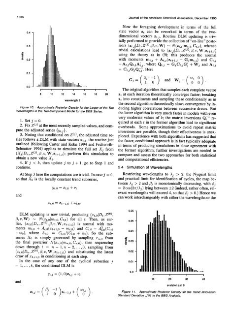I I 0.0 dI IIIIIIIIhh The original algorithm that samples each complete vector 8 10 12 14 16 18 20 zt at each iteration theoretically converges faster; breaking zt wavelength 2 into constituents and sampling these conditionally as in the second algorithm theoretically slows convergence by in- Figure 10. Approximate Posterior Density for the Larger of the Two ducing higher correlations between successive draws. But Wavelengths in the Two-Component Model for the EEG Series. the latter algorithm is very much faster in models with even very moderate values of k; the matrix inversions Q71 re- 1. Set j = 0. quired at each t in the former algorithm lead to significant 2. Fix Z() at the most recently sampled values, and com- overheads. Some approximations to avoid repeat matrix pute the adjusted series {Yt,j}. inversions are possible, though their effectiveness is unex- 3. Noting that conditional on Zi), the adjusted time se- plored. Experience with both algorithms has suggested that ries follows a DLM with state vectors xt,j, the routine just the faster, conditional approach is in fact typically adequate outlined (following Carter and Kohn 1994 and Fruhwirth- in terms of producing simulations in close agreement with Schnatter 1994) applies to simulate the full set Xj from the former algorithm; further investigations are needed to (XjJ Dn, Z zU) 3, v, xW zt+?1,3); perform this simulation to compare and assess the two approaches for both statistical obtain a new value X . and computational efficiencies. 4. If j < k, then update j to j + 1, go to Step 1 and continue. 2.4 Simulation of Wavelengths At Step 3 here the computations are trivial. In case j = 0, Restricting wavelengths to Aj > 2, the Nyquist limit so that Xo is the locally constant trend subseries, and practical limit for identification of cycles, the map between Aj > 2 and 3j is monotonically decreasing, with 3j Yt,o = Xt,O + Vt = 2 cos(2ir/Aj) lying between +2 (indeed, rather often, relevant wavelengths will exceed 4, so that and 3j > 0.) Hence we can work interchangeably with either the wavelengths or the Xt,O = Xt- 1,0 + Wt,O 0.06 - DLM updating is now trivial, producing (xt,o Dt IZ(O) 3, v, W) - N(xt,oJmt,o, Ct,o) for all t. Then, as ear- 0.05 lier, (xt,oJDn,Z(?),3,v,V, xt+1iO) is normal with moments mt,o + At,o(xt+?,o - mt,o) and Ct,o - A 2 o(Ct o 0.04- +wo), where At,o = Ct,O/(Ct,O + wo). So the subseries Xo is simply generated by sampling xn,O from the final 0.03- posterior N(xn,oJMn,O, CT,O), then sequencing down through t = n - 1, n - 2,... , 0, sampling from (Xt,OJDn,Z(0)1)3,v,W,xt+?io) and substituting the latest 0.02- draw of xt+,,o in conditioning at each step. In the case of any one of the cyclical subseries j 0.01 = 1, ... , k, the conditional DLM is Yt,j = (1,0)zt,j+ Vt 10 20 30 40 and evolution s.d. 0 Ztj= (pi; ~o1 )Ztil,3 ? (wti ) - Figure 11. Approximate Posterior Density for the Trend Innovation Standard Deviation +/i in the EEG Analysis.
West: Inference on Cycles in Time Series 1307 0.15 - 0.10 - 0.15 0.05 0.0 1 . 0 10 20 30 evolution s.d. 1 Figure 12. Approximate Posterior Density for the Component Innovation Standard Deviation f/w- in the EEG Analysis. 0.0 _ 0 5 10 15 20 evolution s.d. 2 Figure 13. Approximate Posterior Density for the Component Innovation Standard Deviation vw2 in the EEG Analysis. autoregressive coefficients; simulation of the 3 parameters (8) implies from conditional posteriors p(,3W, Z) in (9) produces sampled wavelengths via the identities Aj = 27r/arccos(ij/2) p(/j3IDn, :(i), v, W, Z) cX N(,3j bj, Bjwj), for each j, and posterior inferences may be explored di- (d( 1 i j+)l rectly from the samples. Conversely, it is natural to think in terms of priors for the wavelengths and then transform So sampling may proceed conditionally, cycling through to deduce priors for the da. the /j parameters given previously sampled values of 3(i) (among other things), with new values of the Strict constraints on wavelengths may be enforced Oj trivially generated from a truncated normals. through the prior distribution. Some form of constraint As noted, other priors might be used, as context deis necessary for identification-note that the model remands, based on transforming from plausible priors for mains the same under arbitrary permutation of the wave- the A3. Working in terms of conditional priors is natural, length indices. The constraint here is simply the ordering and the foregoing development is modified only through A1 < A2 < ... < Ak under the prior, and this provides conditionals p(j[3U(i)) that will be other than uniforms. parameter identification. Other strict constraints, such as The conditional posteriors are then p(j3 IDn, d3(i), v, W, Z) enforcing a minimum separation between any two wave- c< p(Oj3 M(i))N(3jjbj,Bjwj) so the analysis differs only lengths, may be desirable in some applications and can be technically; sampling these conditional posteriors will gensimilarly introduced. In an illustration that follows we use conditional priors that are effectively reference priors for the Oj conditional on all other parameters, simply conditional uni- 0.08- forms. This provides a benchmark analysis. Alternative analyses based on plausible, informed priors for the Aj 0.06- that induce specific forms of priors for the Oj parameters may be similarly implemented within this framework. Write U(. la, b) for the uniform distribution on (a, b) and 0.04 suppose a specified minimum wavelength separation of 6 > 0 time units (e.g., 6 = 1). The class of priors used is defined by the set of complete conditionals (lujj(i)), 0.02 - where :3() = \ ij _ { ,3. ..,/3j-1,/3j+1, . . ,k}, for all j. Extend notation to include fixed and specified lim- its on wavelengths A0 < Ak+l; often Ao = 2 and Ak+1 is some appropriately large value. Then take conditionals (p3ylp(J)) U(p3jl3p~ i34l,(2) for all j, where j) =2 cos(2wr/(Aj_i + 6)) and p3(2)l = 2 cos(2w/(A3+1 - 6)). Under the joint prior so specified, the conditional posterior 0.0 I I I I 20 30 40 50 observation s.d. Figure 14. Approximate Posterior Density for the Observation Error Standard Deviation fv in the EEG Analysis.
Page 1 and 2: Bayesian Inference in Cyclical Comp
Page 3 and 4: West: Inference on Cycles in Time S
Page 5: West: Inference on Cycles in Time S

Bayesian Inference in Cyclical Component Dynamic Linear Models

You also want an ePaper? Increase the reach of your titles

Delete template?

Save as template?