Bayesian Inference in Cyclical Component Dynamic Linear Models

1308 Journal of the American Statistical Association, December 1995
12 +
10 +++;++
61+a 4~~~X + * + + ++ +
co - 8
+
+
+
+ 4+++ +
+ . 4
+
+ + 4? ++I.
+ + +~~~~~~~~
co ~~~~~~~~~~~~++
++~~~~~~~~~~
2
-500 0 500 1000
nominal years AD
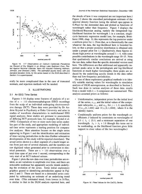
Figure 15. 177 Observations on Calcium Carbonate Prevalence
(as Percent of Dry Weight) in an African Lake Sediment Core, Plotted
Against Nominal Calendar Years AD Imputed Following Halfman,
Johnson, and Showers (1994). The estimated acyclic trend, with one
standard deviation limits, for the series based on the DLM described in
Section 3 is superimposed.
erally be more complicated than in the case of truncated
normals, and rejection methods will be needed.
3.1 An EEG Time Series
3. ILLUSTRATIONS
Figures 1-14 display some features of analysis of a series
of nr= 110 electroencephalogram (EEG) recordings
from the scalp of an individual undergoing electroconvulsive
therapy (ECT). These data were provided by Dr Andrew
Krystal in Psychiatry at Duke University and arise in
studies of waveform characteristics in multichannel EEG
signal analyses; these studies are germane to assessments
of differing ECT protocols (see, for example, Krystal et al.
1992). Comparison of two or more such time series underlies
part of the study, and appropriate modeling of individual
time series represents a starting position for comparative
analyses. Here attention focuses on the single series
appearing in Figure 1 and the identification and estimation
of time-varying periodicities in the data (further substantive
developments of this study will be reported elsewhere). The
actual series shown is a short segment of a much longer series
from just one of several channels, and the numbers are
raw digitized values generated prior to conversion to electrical
potentials. There are nr= 110 observations over a
total time span of just over 1 second, corresponding to the
very start of an ECT-induced seizure.
Figure 1 plots the raw data over time; periodicities are evident,
as are variations in amplitude over time, and there are
noticeable nonlinear but apparently acyclic trends underlying
the evolution of the series. Some initial exploratory
graphics geared to identifying periodicities appear in Figures
2 and 3. These are based on a detrended series computed
by subtracting an estimate of an underlying trend
over time. (This estimated trend, from lowess in S-Plus,
is similar to that in the DLM analysis reported here, and
the details of how it was computed are not important here.)
Figure 2 shows the smoothed periodogram estimate of the
spectral density function (using the default spec.pgram in
S-Plus) for the detrended data and plotted as functions of
wavelength rather than frequency. Figure 3 displays the
likelihood/Bayesian analog, namely the (integrated) loglikelihood
function for wavelength A in a constant, singlecycle
harmonic regression model (see, for example, Bretthorst
1988, chap. 3); this represents the log-posterior under
a uniform prior for A. (Note that, as is theoretically the case
whatever the data, the log-likelihood here is bounded below,
so that a proper posterior distribution is obtained only
under a proper prior for A.) Qualitatively, these figures indicate
high power at wavelengths around A = 6, with some
possible contributions in the wavelength range 10-15. Note
that qualitatively similar conclusions are arrived at using
the raw data, rather than the specific detrended version used
here. The differences are that additional and apparently important
peaks arise in the periodogram and log-likelihood
functions at much higher wavelengths; these peaks are induced
by the underlying acyclic trends in the data rather
than real low-frequency periodicities.
On use of these exploratory graphical methods is to identify
suitable starting values for wavelengths in simulation
analysis of DLM autoregression, as described in Section 2.
Such was done in various analyses of these data; results
from a model with k = 2 component are summarized. This
analysis assumed priors as follows:
* Uninformative, independent priors for the initial level
of the series, x1,0, and the initial values of the component
subcycles, x1,j and xo,j for j = 1, 2; specifically,
N(xi,o10, 1,000) and N(zi 0,1,000I), where I is the
identity matrix.
* Conditionally uniform priors for the wavelength coefficients
3 induced by constraints on wavelengths of
2.0 < A. < 25.0, and a minimum separation of one
wavelength. A2 > A1 + 1.0 (though this turns out to
be nonbinding, as the likelihood function gives little
support to close values of the two wavelengths.)
12 -
J
12J
c~~,8 I~
1I I I I
-500 0 500 1000
nominal years AD
Figure 16. Fitted Values for the CaCO3 Series.