TUTORIAL 2 SOLUTIONS #7.7.11 Consider a population of size four ...
TUTORIAL 2 SOLUTIONS #7.7.11 Consider a population of size four ...
TUTORIAL 2 SOLUTIONS #7.7.11 Consider a population of size four ...

Create successful ePaper yourself
Turn your PDF publications into a flip-book with our unique Google optimized e-Paper software.
<strong>TUTORIAL</strong> 2 <strong>SOLUTIONS</strong><br />
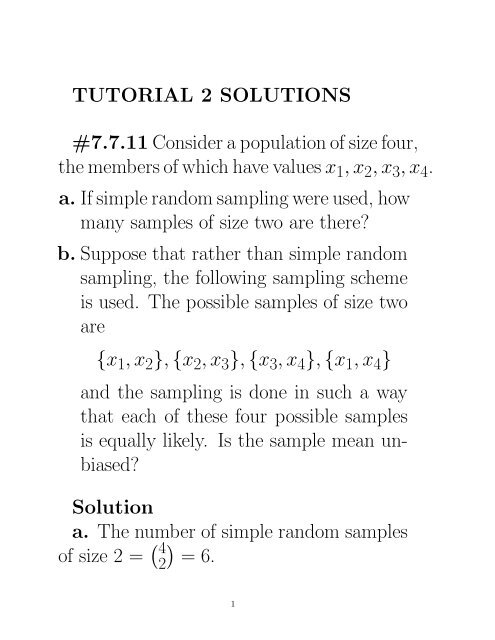
<strong>#7.7.11</strong> <strong>Consider</strong> a <strong>population</strong> <strong>of</strong> <strong>size</strong> <strong>four</strong>,<br />
the members <strong>of</strong> which have values x 1 ,x 2 ,x 3 ,x 4 .<br />
a. If simple random sampling were used, how<br />
many samples <strong>of</strong> <strong>size</strong> two are there?<br />
b. Suppose that rather than simple random<br />
sampling, the following sampling scheme<br />
is used. The possible samples <strong>of</strong> <strong>size</strong> two<br />
are<br />
{x 1 ,x 2 }, {x 2 ,x 3 }, {x 3 ,x 4 }, {x 1 ,x 4 }<br />
and the sampling is done in such a way<br />
that each <strong>of</strong> these <strong>four</strong> possible samples<br />
is equally likely. Is the sample mean unbiased?<br />
Solution<br />
a. The number <strong>of</strong> simple random samples<br />
<strong>of</strong> <strong>size</strong> 2 = ( 4<br />
2<br />
)<br />
=6.<br />
1
. Let µ denote the <strong>population</strong> mean. I.e.<br />
µ = x 1 + x 2 + x 3 + x 4<br />
.<br />
4<br />
We observe that<br />
E( ¯X) = 1 4 [x 1 + x 2<br />
+ x 2 + x 3<br />
2 2<br />
+ x 3 + x 4<br />
+ x 1 + x 4<br />
]<br />
2 2<br />
= x 1 + x 2 + x 3 + x 4<br />
4<br />
= µ.<br />
This implies that the sample mean is an<br />
unbiased estimate <strong>of</strong> the <strong>population</strong> mean<br />
(even though the sample is not a s.r.s.).<br />
2
#7.7.12 <strong>Consider</strong> simple random sampling<br />
with replacement.<br />
a. Show that<br />
s 2 = 1<br />
n − 1<br />
n∑<br />
(X i − ¯X) 2<br />
i=1<br />
is an unbiased estimate <strong>of</strong> σ 2 .<br />
b. Is s an unbiased estimate <strong>of</strong> σ?<br />
c. Show that n −1 s 2 is an unbiased estimate<br />
<strong>of</strong> σ 2¯X.<br />
d. Show that n −1 N 2 s 2 is an unbiased estimate<br />
<strong>of</strong> σ 2 T .<br />
e. Show that ˆp(1− ˆp)/(n−1) is an unbiased<br />
estimate <strong>of</strong> σ 2ˆp .<br />
Solution First we observe that the sample<br />
X 1 ,...,X n is an i.i.d. sequence <strong>of</strong> random<br />
variables.<br />
3
a. Let µ = E(X 1 ) and Y i = X i −µ. Then<br />
E(Y i )=0,<br />
Var(Y i )=Var(X i )=σ 2 ,<br />
E(s 2 )= 1 n∑<br />
E[X<br />
n − 1 i − µ − ( ¯X − µ)] 2<br />
i=1<br />
= 1 n∑<br />
E(Y<br />
n − 1 i − Ȳ )2<br />
i=1<br />
= 1 n∑<br />
E(Y 2<br />
n − 1<br />
i − 2Y iȲ + Ȳ 2 )<br />
i=1<br />
= nσ2<br />
n − 1 −<br />
+ n<br />
n − 1 E(Ȳ 2 )<br />
= nσ2<br />
n − 1 −<br />
2n<br />
n − 1 E(Ȳ 2 )<br />
n<br />
n − 1 E(Ȳ 2 ).<br />
4
Since E(Ȳ 2 ) = Var(Ȳ )=σ2 /n,<br />
E(s 2 )=<br />
nσ2<br />
n − 1 −<br />
= σ 2 .<br />
σ2<br />
n − 1<br />
This implies that s 2 is an unbiased estimate<br />
<strong>of</strong> σ 2 .<br />
b. No, s is not an unbiased estimate <strong>of</strong> σ<br />
since in general<br />
√<br />
E(s) =E(<br />
√<br />
s 2 )<br />
< E(s 2 )<br />
√<br />
= σ 2 = σ.<br />
This follows from Jensen’s inequality and<br />
E(s) = √ E(s 2 ) only if s is a constant.<br />
5
c. From a. we have<br />
E(n −1 s 2 )= 1 n E(s2 )<br />
= σ2<br />
n<br />
= σ 2¯X .<br />
That is n −1 s 2 is an unbiased estimate <strong>of</strong> the<br />
variance <strong>of</strong> ¯X.<br />
d. Recall that T = N ¯X and Var(T )is<br />
given by<br />
Consequently,<br />
σ 2 T<br />
=Var(N ¯X)<br />
= N 2 Var( ¯X)<br />
= N 2σ2<br />
n .<br />
E(n −1 N 2 s 2 )=n −1 N 2 E(s 2 )<br />
= n −1 N 2 σ 2<br />
= σ 2 T .<br />
6
This shows that n −1 N 2 s 2 is an unbiased estimate<br />
<strong>of</strong> σ 2 T .<br />
e. Recall that ˆp = ¯X when the X i ’s only<br />
take values 0 or 1. Observe that<br />
σ<br />
2ˆp = σ2¯X<br />
= σ2<br />
n .<br />
Consequently,<br />
E<br />
ˆp(1 − ˆp)<br />
n − 1<br />
= 1<br />
n − 1 E[1 n<br />
=<br />
1<br />
n(n − 1)<br />
n∑<br />
Xi 2 − ¯X 2 ]<br />
i=1<br />
n∑<br />
E(X i − ¯X) 2<br />
i=1<br />
= 1 n E(s2 )= σ2<br />
n .<br />
This shows that ˆp(1 − ˆp)/(n − 1) is an unbiased<br />
estimate <strong>of</strong> σ 2ˆp . 7
#7.7.23<br />
a. Show that the standard error <strong>of</strong> an estimated<br />
proportion is largest when p =<br />
1/2.<br />
b. Use this result and Corollary B <strong>of</strong> Section<br />
7.3.2 to conclude that the quantity<br />
√<br />
1 N − n<br />
2 N(n − 1)<br />
is a conservative estimate <strong>of</strong> the standard<br />
error <strong>of</strong> ˆp no matter what the value <strong>of</strong> p<br />
may be.<br />
c. Use the central limit theorem to conclude<br />
that the interval<br />
√<br />
N − n<br />
ˆp ±<br />
N(n − 1)<br />
contains p with probability at least 0.95.<br />
8
Solution<br />
a. Recall that the sample is s.r.s. From<br />
page 214 <strong>of</strong> the text, the standard error <strong>of</strong> ˆp<br />
is given by<br />
√<br />
σˆp = ( N − n − p)<br />
)p(1 .<br />
N − 1 n<br />
Treating σˆp as a function <strong>of</strong> p, we note that<br />
f(p) =p(1 − p), 0 ≤ p ≤ 1, is maximized<br />
when p =1/2.<br />
b. Using a. and Corollary B <strong>of</strong> Chapter<br />
7.3.2, we have<br />
ˆp(1 − ˆp)<br />
s<br />
2ˆp =<br />
n − 1 (1 − n N )<br />
≤ 1 2 (1 − 1 2 )( 1<br />
n − 1 )(1 − n N )<br />
= N − n<br />
4N(n − 1) .<br />
9
Taking square root, we have<br />
√<br />
sˆp ≤ 1 N − n<br />
2 N(n − 1) .<br />
The r.h.s. is a conservative estimate <strong>of</strong> the<br />
standard error <strong>of</strong> ˆp.<br />
c. Using the CLT from s.r.s., a 95% CI for<br />
p is<br />
ˆp ± z 0.025 sˆp .<br />
Since z 0.025 =1.96 ≈ 2, it follows from b.<br />
that the interval<br />
ˆp ±<br />
√<br />
N − n<br />
N(n − 1) .<br />
contains p with probability at least 0.95.<br />
10
#7.7.24 For a random sample <strong>of</strong> <strong>size</strong> n<br />
from a <strong>population</strong> <strong>of</strong> <strong>size</strong> N, consider the<br />
following as an estimate <strong>of</strong> µ:<br />
n∑<br />
¯X c = c i X i<br />
i=1<br />
where the c i are fixed numbers and X 1 ,...,X n<br />
is the sample.<br />
a. Find a condition <strong>of</strong> the c i such that the<br />
estimate is unbiased.<br />
b. Show that the choice <strong>of</strong> c i that minimizes<br />
the variance <strong>of</strong> the estimate subject to<br />
this condition is c i = 1/n, where i =<br />
1,...,n.<br />
11
Solution Note that in this problem, a<br />
random sample is meant an i.i.d. sample.<br />
a. ¯Xc is an unbiased estimate <strong>of</strong> the <strong>population</strong><br />
mean µ iff<br />
µ = E( ¯X<br />
n∑<br />
c )= c i E(X i )<br />
=(<br />
i=1<br />
n∑<br />
c i )µ.<br />
i=1<br />
This implies that the condition for unbiasness<br />
is<br />
n∑<br />
c i =1.<br />
i=1<br />
12
. Let Var(X 1 )=σ 2 . Then by the independence<br />
<strong>of</strong> X 1 ,...,X n , we have<br />
Var( ¯X<br />
n∑<br />
c )=Var( c i X i )<br />
=<br />
i=1<br />
n∑<br />
c 2 i Var(X i)<br />
i=1<br />
n<br />
= σ 2 ∑<br />
c 2 i .<br />
i=1<br />
We want to minimize ∑ n<br />
∑ i=1 c 2 i<br />
subject to<br />
ni=1<br />
c i =1.<br />
To do that we minimize the following Lagrangian<br />
function:<br />
n∑<br />
f(c 1 ,...,c n ,λ)= c 2 n i + λ(1 − ∑<br />
c i ).<br />
i=1<br />
i=1<br />
Here λ is the Lagrangian multiplier.<br />
13
We partial differentiate f wrt c 1 ,...,c n ,λ,<br />
∂f<br />
=2c<br />
∂c i − λ, i =1,...,n,<br />
i<br />
∂f<br />
n<br />
∂λ =1− ∑<br />
c i .<br />
i=1<br />
Equating these partial derivatives to 0, we<br />
have<br />
c i = λ 2 , i =1,...,n,<br />
n∑<br />
1=<br />
i=1<br />
= λn 2 .<br />
c i<br />
Solving for c i and λ, we have<br />
λ = 2 n ,<br />
c i = 1 n , i =1,...,n.<br />
14
By taking 2nd partial derivatives <strong>of</strong> f, it<br />
can be shown that this gives the minimum<br />
(and not maximum) <strong>of</strong> f.<br />
15