Classes of Discrete Variable

Multiple Discrete Choice Models 

Classes of Discrete Variable 

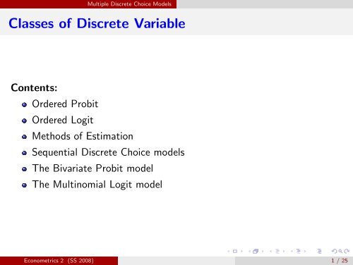
Contents: 

Ordered Probit 

Ordered Logit 

Methods of Estimation 

Sequential Discrete Choice models 

The Bivariate Probit model 

The Multinomial Logit model 

Econometrics 2 (SS 2008) 1 / 25


The Ordered Probit/Logit Model 

Sometimes a simple binary choice model is inappropriate: 

eg. model of labour market status 

degree of satisfaction 

number of cars owned 

Each of these examples involves more than two possible outcomes. 

One possible model specification: the Ordered Probit or Logit 

model: 

appropriate when discrete outcomes have a natural (ordinal) ranking 

major advantage: the resulting model is relatively easy to estimate 

down-side: the behavioural model may be considered too restrictive 




Consider an independent sample of data {y i , x i } of size n. 

Let y i have M possible outcomes y i = m for m = 1, ..., M and 

natural ordering (e.g. m + 1 is in some sense better than m). 

Consider a latent variable y ∗ 

i 

where 

y ∗ 

i = x ′ i β + u i for i = 1, ..., n 

Define the following observability criterion: 

y i = m if α m−1 ≤ y ∗ 

i ≤ α m for m = 1, ..., M, 

α 0 < α 1 < α 2 < ... < α M , 

α 0 = −∞ and α M = ∞ 




The conditional probability of observing y i = m is 

P(y i = m|x i ) = P(α m−1 ≤ y ∗ 

i ≤ α m ) 

= P(α m−1 ≤ x ′ i β + u i ≤ α m ) 

Rearranging gives for m = 1, ..., M 

P(y i = m|x i ) = P(α m−1 − x ′ i β ≤ u i ≤ α m − x ′ i β) 

= P(u i ≤ α m − x ′ i β) − P(u i ≤ α m−1 − x ′ i β) 

Need a distribution for u i 

u i std normal gives the Ordered Probit 

u i logistic gives the Ordered Logit 



Ordered Probit: graphical representation 

eg. let u i ∼ N(0, 1). Then 

P(y i = m|x i ) = Φ(α m − x ′ i β) − Φ(α m−1 − x ′ i β) 


Estimation 


Estimate this non-linear model by maximum likelihood: 

let z im = 1I(y i = m), for m = 1, ..., M, 

then the ith likelihood contribution is 

L i = 

= 

M∏ 

P(y i = m|x i ) z im 

m=1 

M∏ 

[Φ(α m − x i ′ β) − Φ(α m−1 − x i ′ β)] z im 

. 

m=1 

The full likelihood function becomes 

L(α, β) = 

n∏ 

i=1 m=1 

M∏ 

[Φ(α m − x i ′ β) − Φ(α m−1 − x i ′ β)] z im 

. 



Estimation 

Taking logs, 

l = 

n∑ M∑ 

z im ln[Φ(α m − x i ′ β) − Φ(α m−1 − x i ′ β)]. 

i=1 m=1 

For ML estimates, solve 

discuss conditions 

discuss consequences 

∂l 

∂α = 0 and ∂l 

∂β = 0. 



The Sequential Probit/Logit model 

What if decisions / alternatives are not independent? 

Take as an example a sequential decision rule: 

Can be used when dependent variable can be separated into a 

sequence of binary choices. 

For the simplest sequential model, we also assume u i independent. 

Some examples: 



Sequential Probit/Logit model: Example 1 

labour force status 



Sequential Probit/Logit model: Example 2 

transport mode 



Sequential Probit/Logit model 

Consider a sample of data {y 0i , y 1i , x i , z i }. 

Let y 0i represent a binary indicator variable for some discrete choice. 

Let y 1i represent a second discrete choice, observed only when 

y 0i = 1. 

Let the k 0 explanatory variables x i influence the first choice. 

Let the k 1 explanatory variables z i influence the conditional choice. 

For the first stage, assume with u 0i ∼ N(0, 1) iid 

y ∗ 0i = x ′ i β 0 + u 0i 



Sequential Probit/Logit Model 

Observe y 0i = 1I(y0i ∗ > 0). 

Hence P(y 0i = 1|x i ) = Φ(x 

i ′ β 0). 

Estimation by standard Probit MLE on the full sample. 

For the second stage, note first that 

P(y 0i = 1, y 1i = 1) = P(y 0i = 1) ∗ P(y 1i = 1|y 0i = 1). 

Hence, select a sample of the n 1 observations for which y 0i = 1. 

Define for u 1i ∼ N(0, 1) iid 

y ∗ 1i = z ′ i β 1 + u 1i 



Sequential Probit/Logit Model 

For the second stage y 1i = 1I(y1i ∗ > 0). So, 

P(y 1i = 1|z i ) = Φ(z i ′ β 1 ). 

Estimation by standard Probit MLE on the selected sample. 

The overall probabilities of the three possible outcomes are 

P(y 0i = 0|x i ) = 1 − Φ(x i ′ β 0 ) 

P(y 0i = 1, y 1i = 0|x i , z i ) = Φ(x i ′ β 0 ) ∗ [1 − Φ(z i ′ β 1 )] 

P(y 0i = 1, y 1i = 1|x i , z i ) = Φ(x i ′ β 0 ) ∗ Φ(z i ′ β 1 ) 

Upside: easy to estimate 

Downside: ignores a potential correlation between u 0i and u 1i . 



The Bivariate Probit Model 

Binary decisions may form part of a system of choices rather than a 

sequence, eg. simultaneous decisions of work and take-up of paid 

childcare. 

Can apply the Bivariate Probit in these circumstances: 

Consider {y 0i , y 1i , x 0i , x 1i } for i = 1, ..., N. 

Here, y 0i and y 1i represent two binary indicator variables. 

Assume an underlying system of propensities: 

y ∗ 0i = x ′ 0iβ 0 + u 0i , 

y ∗ 1i = x ′ 1iβ 1 + u 1i . 



The Bivariate Probit Model 

The observability criteria: 

y 0i = 1I(y ∗ 0i > 0), 

y 1i = 1I(y ∗ 1i > 0). 

For a Bivariate Probit model, u 0i and u 1i are bivariate normal: 

1 

φ 2 (u 0 , u 1 ; ρ) = 

2π(1 − ρ 2 ) 1 2 

Φ 2 (u 0 , u 1 ; ρ) = 

∫ u1 

−∞ 

∫ u0 

−∞ 

∗ exp(− u2 0 + u2 1 − 2ρu 0u 1 

1 − ρ 2 ) 

φ 2 (u, v; ρ)∂u∂v 

Note that when ρ = 0, Φ 2 (u 0 , u 1 ; 0) = Φ(u 0 ) ∗ Φ(u 1 ). 



Estimating a Bivariate Probit 

Derive probabilities P jk for j, k = 0, 1. 

For example, 

P 00i = P(y 0i = 0, y 1i = 0|x 0i , x 1i ) 

= P(y0i ∗ ≤ 0, y1i ∗ ≤ 0|x 0i , x 1i ) 

= P(u 0i ≤ −x 0iβ ′ 0 , u 1i ≤ −x 1iβ ′ 1 ) 

= Φ 2 (−x 0iβ ′ 0 , −x 1iβ ′ 1 ; ρ). 

Similarly, 

P 11i = P(y 0i = 1, y 1i = 1|x 0i , x 1i ) = Φ 2 (x 0iβ ′ 0 , x 1iβ ′ 1 ), 

P 01i = P(y 0i = 0, y 1i = 1|x 0i , x 1i ) = Φ(x 1iβ ′ 1 ) − P 11i , 

P 10i = P(y 0i = 1, y 1i = 0|x 0i , x 1i ) = Φ(x 0iβ ′ 0 ) − P 11i . 




Contours of the bivariate normal distribution 




Bivariate Probit probabilities 




Estimation then follows by ML: 

L(β, ρ) = 

Taking logs, 

N∏ 

i=1 

P (1−y 0i )(1−y 1i ) 

00i 

ln L(β 0 , β 1 , ρ) = 

∗ P (1−y 0i )y 1i 

01i 

∗ P y 0i (1−y 1i ) 

10i 

∗ P y 0i y 1i 

11i 

N∑ 

{(1 − y 0i )(1 − y 1i ) ln P 00i 

i=i 

+ (1 − y 0i ) ∗ y 1i ln P 01i 

+ y 0i ∗ (1 − y 1i ) ∗ ln P 10i 

+ y 0i ∗ y 1i ∗ ln P 11i }. 



The Multinomial Logit Model 

Simplest model for unordered discrete choices 

where covariates do not vary with m. 

Example: public transport choice. 

Consider M discrete alternatives 

P mi = P(y i = m) for m = 1, ..., M. 

Thinking again of latent variables, here utilities; 

U ∗ im = x ′ i β m + u im 

we get 

P mi = P ( U ∗ im > U ∗ ij, ∀j ≠ m ) 




Let us derive the probability model generally: 

For the Multinomial Model , m = 1, ..., M − 1 

for a benchmark probability P M . 

This implies that 

P m 

P m + P M 

= F (x ′ β m ) 

P m 

P M 

= F (x ′ β m ) 

1 − F (x ′ β m ) = λ(x ′ β m ) 

would reminds us of the logit distribution. 

Will see that F (·) is cdf 




Since P m ∈ (0, 1), we therefore have that 

P m 

→ 0 

P m + P M 

as P m → 0, 

P m 

→ 1 

P m + P M 

as P m → 1. 

So, F (.) is a monotone increasing function, 

F (u) → 0 as u → −∞, 

F (u) → 1 as u → ∞. 

Since ∑ M 

m=1 P m = 1, we have that 

M−1 

∑ 

j=1 

P j 

P M 

= 1 − P M 

P M 

= 1 

P M 

− 1. 




Hence, for all m = 1, ..., M − 1 

M−1 

∑ 

M−1 

P j 

∑ 

P M = [1 + ] −1 = [1 + λ(x ′ β j )] −1 

P M 

P m = 

j=1 

λ(x ′ β m ) 

1 + ∑ M−1 

j=1 λ(x ′ β j ) 

General derivation (one possibility), 

for the MLM we set λ(u) = exp(u). 

Alternatives are possible but rarely used. 

j=1 

Suffers from certain restrictions, maybe most crucial: 



The Independence of Irrelevant Alternatives 

Recall the formulae for the probabilities, 

for all m = 1, ..., M − 1. 

However, looking at 

P m = 

exp(x ′ β m ) 

1 + ∑ M−1 

j=1 exp(x ′ β j ) 

P j 

= exp(x ′ β j ) 

P k exp(x ′ β k ) . 

we notice that this ratio is independent of the probability of any other 

outcome. 

This is called the assumption of independence of irrelevant 

alternatives. Now, compare this with sequential decisions. 



The Conditional Logit Model 

still unordered discrete choices 

now covariates may vary over m 

Example: distance to store. 

Consider M discrete alternatives 

P mi = P(y i = m) for m = 1, ..., M. 

Thinking again of latent variables, here utilities; 

U ∗ im = x ′ imβ + u im 

β fixed for identification. Again we have 

P mi = P ( U ∗ im > U ∗ ij, ∀j ≠ m ) 

Have no benchmark, similar derivation leads to 

P mi = 

exp(x ′ im β) 

∑ M 

j=1 exp(x ′ ij β)

Classes of Discrete Variable

Create successful ePaper yourself

Delete template?

Save as template?