Casestudie Breakdown prediction Contell PILOT - Transumo

Technische Universität Braunschweig
Diplomarbeit
AUSFALLPROGNOSEN MIT HILFE
ERWEITERTER MONITORING SYSTEME
(Breakdown Prediction by the Use of Extended Monitoring Systems)
von
Christian Kaak
Februar 2007
Institut für Wirtschaftswissenschaften,
Lehrstuhl für Betriebswirtschaftslehre,
insbesondere Produktion und Logistik
Technische Universität Braunschweig
Prüfer:
Prof. Dr. T. Spengler
Betreuer:
Dr. Grit Walther

Table of Contents
Index of Figures...............................................................................................................................IV
Index of Tables.................................................................................................................................V
Index of Formulas............................................................................................................................VI
1 Introduction................................................................................................................................ 1
1.1 Initial Position and Problem ............................................................................................. 1
1.2 Goals of this Study and Approach................................................................................... 1
2 Sensor Based Temperature Monitoring.................................................................................... 3
2.1 Importance of Temperature Monitoring within Medical Laboratories.............................. 3
2.2 Functioning and Behavior of Freezers and Fridges ........................................................ 4
2.2.1 General Functioning of a Fridge.................................................................................. 4
2.2.2 Technical Behavior of Fridges (Without External Influences)..................................... 5
2.2.3 Technical Behavior of Freezers (Without External Influences)................................... 6
2.2.4 Behavior in Practice..................................................................................................... 7
2.2.5 Behavior in Case of a Malfunction............................................................................... 9
2.3 Current Practice of Sensor Based Temperature Monitoring......................................... 10
2.4 Problems and Potential Sources of Error...................................................................... 11
2.4.1 The Lack of Information Problem .............................................................................. 12
2.4.2 Potential Sources of Error ......................................................................................... 14
2.4.3 Methodological Problems .......................................................................................... 15
2.5 Aimed Goal and Requirements Analysis....................................................................... 16
3 Current Monitoring Systems ................................................................................................... 19
3.1 XiltriX’s Technical Basis................................................................................................. 19
3.1.1 Basic Components of a XiltriX Installation ................................................................ 21
3.1.2 Other Installation Possibilities ................................................................................... 22
3.2 XiltriX’s Basic Functionality............................................................................................ 23
3.2.1 Current Possibilities to Display and Analyze Stored Data ........................................ 26
3.2.2 Documentation of Occurred Alarms .......................................................................... 30
3.3 XiltriX’s Additional Features........................................................................................... 31
3.3.1 Different Types of Attachable Digital Switches ......................................................... 31
3.3.2 Time-Dependent Limit Settings................................................................................. 32
3.3.3 Alarm-, SMS- and E-Mail-Programs.......................................................................... 33
3.4 Review of XiltriX According to the Requirements Analysis........................................... 35
3.5 Other Major Monitoring Products in the Market ............................................................ 36
3.5.1 3M FreezeWatch and 3M MonitorMark Indicators............................................. 37
3.5.2 2DI ThermaViewer..................................................................................................... 38
3.5.3 Systems Offering Data Analysis in Retrospect ......................................................... 39
4 Current State of Research ...................................................................................................... 43
4.1 Current State within the Setting of Sensor Based Temperature Monitoring................. 43
4.2 Current State within the Setting of Machinery Condition Monitoring ............................ 43
4.3 Current State within the Setting of Measurement Data Analysis .................................. 46
4.3.1 Basic Approaches...................................................................................................... 46
4.3.2 A Generalized Approach ........................................................................................... 47
II

4.4 Review of Current State of Research............................................................................ 53
5 Possible and Promising Ways of Data Analysis..................................................................... 55
5.1 The Six Possible Levels of Data Analysis ..................................................................... 55
5.2 Different Kinds of Statistical Analysis............................................................................ 57
5.3 Basic Descriptive Statistical Measures.......................................................................... 58
5.4 Regression..................................................................................................................... 60
5.4.1 The Determination of Regression Functions............................................................. 61
5.4.2 The Major Problems of Regression........................................................................... 63
5.5 Time Series Analysis ..................................................................................................... 65
5.6 Failure- and Availability Ratios ...................................................................................... 67
5.7 Markov Chains............................................................................................................... 68
5.8 Inferential Statistics........................................................................................................ 72
5.9 Data Mining.................................................................................................................... 73
5.9.1 General Fields of Application .................................................................................... 73
5.9.2 Artificial Neural Networks .......................................................................................... 75
5.9.3 Non-Applicability of Artificial Neural Networks to Current Datasets ......................... 78
5.10 Promising Analyzing Methods ....................................................................................... 79
5.10.1 Promising Appliance of Basic Descriptive Statistics............................................. 79
5.10.2 Detection of Changes in Behavior by the Use of Regression............................... 81
5.10.3 Classification by Using Past Behavior .................................................................. 82
5.10.4 Review................................................................................................................... 83
6 Implementation and Case Study............................................................................................. 86
6.1 Implementation of Promising Analyzing Methods ......................................................... 86
6.2 Case Study .................................................................................................................... 89
6.2.1 Detection of Changes in Behavior by Using Descriptive Statistics........................... 90
6.2.2 Detection of Changes in Behavior by the Use of Regression................................... 98
6.2.3 Classification of Alarms by the Use of Historical Data.............................................. 99
6.3 Review ......................................................................................................................... 101
6.4 Recommendations....................................................................................................... 102
7 Summary............................................................................................................................... 105
Bibliography.................................................................................................................................. 107
Appendix 1 – Implementation of Interpolation.............................................................................. 111
Appendix 2 – Implementation of Statistical Methods................................................................... 115
Appendix 3 – Implementation of Data Mining Methods ............................................................... 127
Erklärung (Statement) .................................................................................................................. 134
III

Index of Figures
Figure 2-2: Temperature Sequence of a Properly Working 6°C Passive Fridge [DEMO06]........... 5
Figure 2-3: Temperature Sequence of a Properly Working 6°C Active Fridge [DEMO06] ............. 6
Figure 2-4: Temperature Sequence of a -80°C Active Freezer [DEMO06]..................................... 7
Figure 2-5: Temperature Sequence of a -80°C Passive Freezer [DEMO06] .................................. 8
Figure 2-6: Temperature Sequence of a -20°C Active Freezer [DEMO06]..................................... 8
Figure 2-7: Temperature Sequence of a Cryogenic Freezer in Practical Use [UMC06] ................. 9
Figure 2-8: Lack of Information Problem Caused by Sensor Based Temperature Monitoring ..... 13
Figure 2-9: The Problem of Unknown Behavior between Two Single Data Points....................... 13
Figure 2-10: Estimated Answers of Statistics and Data Mining..................................................... 17
Figure 3-1: Flowchart of the Temperature Monitoring Task .......................................................... 20
Figure 3-2: XiltriX - Schematic Drawing of an Installation with Basic Components ...................... 22
Figure 3-3: XiltriX - The Main Screen [DEMO06]........................................................................... 24
Figure 3-4: XiltriX - Stored Data in Table Form [DEMO06] ........................................................... 27
Figure 3-5: XiltriX - Stored Data in Graphical Form [DEMO06]..................................................... 28
Figure 3-6: XiltriX – Available Statistical Information [DEMO06]................................................... 29
Figure 3-8: XiltriX - Time Dependent Limit Settings [DEMO06]..................................................... 33
Figure 3-9: XiltriX - Setting up an Alarm Relay [DEMO06] ............................................................ 34
Figure 3-13: Centron - A Sample Graph with Multiple Scales [Rees06] ....................................... 42
Figure 4-1: General Overview of the Generalized Approach ([Daßler95], p. 22) (adapted) ......... 48
Figure 4-2: A Delayed Trend Recognition Due to Removal of "Outliers" ...................................... 49
Figure 5-1: Two Samples of Regression ([Bourier03], p. 167) (adapted)...................................... 61
Figure 5-2: Incorrect Regression Function due to an Outlier ([Eckey02], p. 180) (adapted) ........ 63
Figure 5-3: Correct Regression Function ([Eckey02], p.180) (adapted)........................................ 63
Figure 5-4: Sales of an Industrial Heater [Chatfield04].................................................................. 66
Figure 5-5: Sample Transition Probability Graph........................................................................... 70
Figure 5-6: Functioning of an Artificial Neuron ([Hagen97], p. 8) (adapted).................................. 76
Figure 6-1: Exported XiltriX Data (An Excerpt) .............................................................................. 86
Figure 6-2: Temperature Overview of the Selected Sample Dataset............................................ 89
Figure 6-3: Maximum Values at Daytime....................................................................................... 91
Figure 6-4: Maximum Values at Nighttime..................................................................................... 91
Figure 6-5: Minimum Values at Daytime........................................................................................ 93
Figure 6-6: Minimum Values at Nighttime...................................................................................... 93
Figure 6-7: Mean Values at Daytime.............................................................................................. 94
Figure 6-8: Mean Values at Nighttime ........................................................................................... 94
Figure 6-9: Standard Deviation at Daytime.................................................................................... 95
Figure 6-10: Standard Deviation at Nighttime................................................................................ 95
Figure 6-11: Daily Door Openings and Temperature Distribution of the Selected Dataset .......... 98
Figure 6-12: Regression Function for the Selected Dataset.......................................................... 99
IV

Index of Tables
Table 2-1: Error of First and Second Kind ..................................................................................... 12
Table 3-1: Listing of Existing Table Color Codes and Their Meaning ........................................... 25
Table 3-2: Listing of Existing Status bar Color Codes and Their Meaning.................................... 26
Table 3-3: Compliance of XiltriX According to the Requirements Analysis................................... 36
Table 3-4: Compliance of 3M Indicators According to the Requirements Analysis................... 38
Table 3-5: Compliance of the 2DI ThermaViewer According to the Requirements Analysis........ 39
Table 4-1: Compliance of the Generalized Approach According to the Requirements Analysis .. 54
Table 5-1: Estimated Improvements .............................................................................................. 85
Table 6-1: Import Problems of Tested Software Products............................................................. 86
Table 6-2: The Chosen Deltas ....................................................................................................... 96
Table 6-3: Reported Notifications (Based on Nighttime Data)....................................................... 97
Table 6-4: Classification of Alarms............................................................................................... 100
Table 6-5: Results of Classification According to Single Criterions............................................. 100
Table 6-6: Achieved Improvements ............................................................................................. 102
V

Index of Formulas
Formula 4-1: Threshold Value to Determine Potential Outliers..................................................... 49
Formula 4-2: Calculation of Noise.................................................................................................. 51
Formula 4-3: Calculation of Curve Stability.................................................................................... 52
Formula 4-4: Calculation of Prediction Stability ............................................................................. 52
Formula 5-1: The Median Formula................................................................................................. 59
Formula 5-2: The Arithmetic Mean Formula .................................................................................. 59
Formula 5-3: The Standard Deviation Formula.............................................................................. 60
Formula 5-4: Method of Least Squares ......................................................................................... 61
Formula 5-5: Method of Least Squares for an Assumed Linear Trend ......................................... 62
Formula 5-6: Regression Function for Describing Linear Trend.................................................... 62
Formula 5-7: Coefficient of Determination ..................................................................................... 64
Formula 5-8: The Additive Component Model ............................................................................... 66
Formula 5-9: The Multiplicative Component Model ....................................................................... 66
Formula 5-10: The Definition of Availability [Masing88]................................................................. 68
Formula 5-11: The Markov Property .............................................................................................. 68
Formula 5-12: Transition Probability Matrix ................................................................................... 69
Formula 5-13: Conditions for the Transition Probability Matrix...................................................... 69
Formula 5-14: Sample Transition Probability Matrix...................................................................... 70
Formula 5-15: Transition Probabilities of Several Changes in a Row........................................... 70
Formula 5-16: Formula of Chapman-Kolmogorov ......................................................................... 70
Formula 5-17: Formula of Chapman-Kolmogorov (Simplified Version)......................................... 71
Formula 5-18: Identity Matrix as an Example of a non Converging Markov Chain....................... 71
Formula 5-19: Definition of Neurons .............................................................................................. 75
Formula 5-20: Definition of V and F ............................................................................................... 76
Formula 5-21: Determination of Error ............................................................................................ 77
Formula 5-22: The Delta Rule........................................................................................................ 78
Formula 5-23: Hebb Learning Rule................................................................................................ 78
Formula 6-1: Regression Function and Coefficient of Determination............................................ 98
VI

1 Introduction
1.1 Initial Position and Problem
As more and more technical devices do “mission critical” tasks within industry and
medical research, monitoring of such devices is becoming increasingly important.
Possible malfunctions could damage these expensive products or its contents, which
can lead to very high costs (both direct and indirect costs; so called collateral
damage). That is why electronic sensor based monitoring systems have become
popular during the last years.
One of these systems is XiltriX, a hard- and software combination from the company
Contell/IKS, which is currently applied to laboratory equipment. The basic
functionality is to monitor and to record temperature of fridges and/or CO 2
concentration within incubators to prevent damage of goods, stored in these devices.
Elementary functionalities as well as some useful tools are already implemented. The
customer or Contell/IKS defines critical minimum and maximum temperature limits
and as soon as a value is exceeded, the system warns by means of E-Mail or SMS.
The main question is now in which direction the development of the software should
continue. The idea of this study is to extend the existing “reactive” XiltriX to a more
“pro-active” system that recognizes trends and notifies a person in charge before
minimum and maximum critical temperature limits are exceeded. In addition to that,
XiltriX should offer additional decision support to allow a person in charge to better
classify the system’s condition within situations of exceptional temperature levels.
After comparing XiltriX to other major monitoring products, this diploma thesis will
work out some promising ideas to show the possibilities for further development. The
main focus is the recorded monitoring data as currently obtained from the field by
XiltriX. At the moment this data is only accessible numerically or in form of a graph.
Analyzing the graphs manually in retrospect already helped to predict malfunctions,
but the results rely on experience and especially instinct of Contell/IKS staff. At
present it is not clear how reliable this intuitive data analysis really is. It is also
problematic that with this kind of data analysis even an experienced person needs a
lot of time, because graphs from every single sensor have to be looked at manually.
1.2 Goals of this Study and Approach
The main task of research is now to determine, whether and in which way it is
possible to reliably predict malfunctions and to give decision support to the customer.
1

Therefore, statistical and data mining methods shall be applied to currently available
datasets.
Hence, existing customer data has to be collected and analyzed. Furthermore, above
mentioned methods have to be evaluated on their feasibility to offer additional
decision support and to reliably predict malfunctions. This study will stick to the data
currently monitored by sensors in the field and will add no new measurement data.
Moreover, it is necessary to point out the increase in value for the customer for the
found solutions.
First step of research is to define what monitoring is about and to explain its general
importance, current practice, existing problems and a requirements analysis of a
monitoring system within the setting of sensor based temperature monitoring of
fridges. This is done in chapter 2. Afterwards a review of XiltriX and other major
monitoring products is given in chapter 3 to point out the level of compliance with the
worked out requirements. The succeeding chapter 4 will review the current state of
research.
Based on these results in combination with literature research, chapter 5 introduces
suggestions, in which way the system could be improved. Aimed results are:
1. To gain additional knowledge of the cooling device’s condition from recorded
datasets to offer additional decision support in case of an exceptional
temperature level
2. To offer a software that reliably predicts upcoming malfunctions
Offering additional knowledge to the customer, regarding the equipment’s condition,
leads to the idea to determine, what important information could be retrieved from
currently recorded datasets. Therefore, statistical and data mining methods are
evaluated on being able to offer additional information. This evaluation contains
questions like:
• Which statistical methods can be applied?
• What knowledge gain do they offer?
• What are the benefits for the operational staff?
A determination whether the possible knowledge gain is sufficient to also reliably
predict upcoming malfunctions and a succeeding case study will conclude this study.
2

2 Sensor Based Temperature Monitoring
This diploma thesis focuses on sensor based temperature monitoring of freezers and
fridges within medical laboratories. Due to the functioning of a fridge and insufficient
data of a high quantity of possible external influences, this setting is faced with
particular problems. The Dutch company Contell/IKS supported this thesis by
providing a lot of information about their sensor based monitoring system XiltriX.
Moreover, Contell/IKS rendered interviews with several employees of the UMC St.
Radboud (University hospital of Nijmegen, the Netherlands) possible. This customer
also provided stored historical data, which enables a validation of promising
analyzing methods.
Based on the interview’s results, this chapter will highlight the importance of sensor
based temperature monitoring of cooling devices within medical laboratories.
Furthermore, typical behaviors of cooling devices as well as currently applied
monitoring methods are introduced. The identification of possible problems and a
requirements analysis for a perfect working monitoring system conclude this chapter.
2.1 Importance of Temperature Monitoring within Medical
Laboratories
As already pointed out in the last chapter, sensor based temperature monitoring
becomes increasingly important within many different settings. Its task is to reliably
determine the condition of monitored devices. In general, a monitored device should
meet the following criteria to be classified as OK [Weerdesteyn06]:
1. Current state is within predefined specifications
2. General behavior did not change significantly on the short-run
3. General behavior did not change significantly on the long-run
4. Presumably the behavior will not change significantly in the future
Such a classification is very important, because a lot of medical goods have to be
kept cool. Blood samples, for example, need a constant temperature of about 6°C.
Changes in temperature for a longer time are dangerous to these blood samples.
Even more critical are cryogenic fridges. Their samples are stored at -80°C or even
cooler. A freezer’s malfunction can destroy these samples within a very short time.
That has to be avoided because most of them are part of research work and
irrecoverable. The contents of a fridge normally range in age from a few days to more
than thirty years. That is why a breakdown of a freezer can lead to a loss of more
3

than half a million Euro. As a result, a possible breakdown has to be recognized as
soon as possible to be able to save the contents to other devices. [Nijmegen06]
Very important to know is that events like this cannot be insured because of the high
risk. Therefore, many medical laboratories and especially hospitals are very
interested in an intelligent monitoring solution, which is able to recognize upcoming
failures. [Weerdesteyn06]
2.2 Functioning and Behavior of Freezers and Fridges
In order to develop new or improve existing sensor based monitoring approaches,
this section will introduce mandatory knowledge of the functioning and the behavior
of cooling devices.
2.2.1 General Functioning of a Fridge
Although different kinds of cooling devices with different technology do exist, they are
all based on the same idea, the cooling cycle. Figure 2-1 illustrates the cooling cycle
of a regular household refrigerator. The basic idea of this cycle is to transport heat
energy from the inside to the outside of a fridge.
4
2
1 3
Figure 2-1: Cooling Cycle of a
Household Refrigerator (adapted)
[UniMunich06]
The exemplary cycle on the left uses a
compressor. Within this cycle there is a refrigerant.
It reaches the compressor (4) vaporized. The
compressor compresses the gas within the
condenser coil (1). Because of the generated high
pressure, the vaporized refrigerant becomes liquid
and emits heat. After cooling down, the refrigerant
passes the expansion valve (2). The second half of
the cycle is called evaporator coil (3). Within this
low pressured part the liquid refrigerant starts to
vaporize again. Therefore, energy is needed. It is
taken from the air inside the fridge, so that the
inside is cooling down. This vaporized refrigerant
reaches the compressor and the cycle starts again. [UniMunich06]
Fridges with a cooling cycle like that are called active fridges. Within laboratories and
the industry a second class of fridges does exist. These devices do not have an own
4

compressor. They are served by a centralized unit with cold air. Devices like that are
called passive fridges.
2.2.2 Technical Behavior of Fridges (Without External Influences)
Due to the just described functioning, active cooling devices as well as passive ones
do not have a constant temperature. In fact, they warm up a bit, start cooling down
until they are cold enough to turn off again. Depending on the kind of cooling device,
the temperature sequence looks differently. This technical behavior will be
exemplified with some temperature sequences of different kinds of cooling devices to
receive an impression of possible behavior.
These examples were taken from the Contell/IKS XiltriX demo system, which was
built up for testing and presentation purposes. This system monitors some demo
fridges 24/7. As these fridges are normally empty and the doors are kept close, the
collected data offers an overview of typical behavior without external influences.
Figure 2-2 pictures a temperature sequence of a properly working 6°C passive fridge
of about eighteen hours. Most of the time, temperature oscillates between 4°C and
6°C. Moreover, nearly every cooling cycle takes about twenty minutes of time.
Figure 2-2: Temperature Sequence of a Properly Working 6°C Passive Fridge [DEMO06]
Figure 2-2 contains three eye-catching cycles. The first two are between 16 and 18
o’clock. One cycle the fridge cools down, although the upper limit of 6°C is not
reached. Three cycles later the fridge heats up to more than 7°C. The last suspicious
cycle is around 2 o’clock in the morning. The fridge reaches a temperature of 6.8°C
before it starts to cool down again.
5

As the following graphs from other machines will show, a behavior like this has to be
classified as normal. Every fridge behaves “suspiciously” sometimes without really
malfunctioning. Actually, machines of the same type behave differently. Also fridges
identical in construction could show different behavior for unknown reason. 1
Figure 2-3: Temperature Sequence of a Properly Working 6°C Active Fridge [DEMO06]
Figure 2-3 shows a temperature sequence of an active fridge. Just like the previous
passive one, it should have a temperature of 6°C. In comparison to each other, the
active fridge never exceeded 6°C within the shown two days. In contrast, the passive
fridge exceeded 6°C about every 20 minutes. Another difference can be found in the
shape of the graph. Figure 2-2 shows a more regular shape with very short cooling
cycles. This is typical for a passive fridge. Figure 2-3 does not contain such a regular
pattern. The cooling cycles are similar but vary in shape. Also the duration of the
passive fridge’s cooling cycle is more than twice as short as the one from the active
device, which is about 43 minutes.
Most results of this comparison cannot be generalized because counterexamples do
exist [DEMO06]. The only indication for a passive fridge is the regular pattern with
very short cooling cycles and a larger deviation. All other differences could be the
other way round when comparing two other 6°C fridges. 2
2.2.3 Technical Behavior of Freezers (Without External Influences)
Looking at freezers even complicates the situation. Figure 2-4 pictures the
temperature sequence of a -80°C active freezer. Although it operates slightly above
1 Reasons are unknown because of the lack of information problem. (See section 2.4.1 for details)
2 See [DEMO06], [UMC06] for further details
6

the specified value, it works very accurately because total deviation is less than 2°C
within the displayed time of five days. On the other hand, the graph contains a trend.
Within four days the daily mean increased more than half a degree. An event like this
has to be recognized and surveyed, when classifying the system’s behavior.
Figure 2-4: Temperature Sequence of a -80°C Active Freezer [DEMO06]
Figure 2-5 shows the behavior of a -80°C passive freezer. This one behaves totally
different. The data does not contain a trend but oscillates much more than the one
above. Furthermore, -80°C is never reached and total deviation is more than 8°C, so
that temperature exceeds -70°C regularly.
Figure 2-6 shows another kind of freezer. The red lines signalize door openings. The
special thing about that device is that it needs a regeneration cycle every few hours
due to technical reasons. Compared to the previous datasets, the oscillation is much
higher and the shape of the graph is more irregular. But as this is normal behavior for
this kind of freezer, it should be classified as OK.
2.2.4 Behavior in Practice
As mentioned at the beginning of this section, the exemplified temperature
sequences originate from the Contell/IKS demo system so far. Since these monitored
cooling devices are empty and not in use, they are not externally influenced by users.
In practice, a cooling device can be influenced by a large quantity of variables. 3
3 See section 2.4.2 for details
7

Figure 2-5: Temperature Sequence of a -80°C Passive Freezer [DEMO06]
Figure 2-6: Temperature Sequence of a -20°C Active Freezer [DEMO06]
Hence, the temperature sequence of a corresponding monitored cooling device
changes to a more irregular pattern. Types and origins of external influences will be
identified in section 2.4.2. Up to then, the following example should just give a
general idea of temperature sequences in practice.
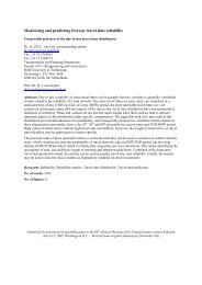
Figure 2-7 shows the behavior of a properly working cryogenic -180°C freezer in
practice. The data originates from the UMC St. Radboud (University hospital of
Nijmegen, the Netherlands) and represents typical behavior for that kind of devices. 4
In contrast to previous examples, this figure pictures a larger time slice. These ten
months are chosen to give an impression of practical behavior on the long run.
Recognizable is a baseline at about -183°C. Due to the different scaling, the figure
does not picture the single cooling cycles any more, although they do exist. Instead
4 The university hospital of Nijmegen provided their datasets only as a copy from their XiltriX system.
That is, why Matlab was used to draw this graph. Beside the slightly different appearance, the data
would look the same in Xiltrix.
8

of this, over a hundred irregular peaks are pictured that cannot be traced back to
typical technical behavior. In fact, not a single peak is caused by a technical
malfunction [Nijmegen06]. Hence, monitoring systems have to be able to figure out,
whether such a peak is caused by a technical malfunction or by external influences.
Figure 2-7: Temperature Sequence of a Cryogenic Freezer in Practical Use [UMC06]
2.2.5 Behavior in Case of a Malfunction
Unfortunately, the provided 36 datasets of the UMC St. Radboud do not contain a
single technical malfunction [UMC06], [Nijmegen06]. In fact, most cooling devices
operate for years without having a single failure, which leads to a very low probability
of a technical malfunction. Hence, it is not possible to introduce a sample pattern
here. Nevertheless, the following criteria are identified to hint a malfunction in case of
not being influenced externally [Weerdesteyn06]:
1. Form and shape of the temperature sequence changes significantly on the
short-run
2. Form and shape of the temperature sequence changes significantly on the
long-run
3. Temperature exceeds the range of normal operation
9

A temperature exceeding without external influence is a definite indication of a
cooling device’s malfunction. But most technical failures are caused by compressor
breakdowns. Usually, such a breakdown does not appear suddenly but predictable
because form and shape of the corresponding temperature sequence starts to
diversify, before the compressor actually breaks down. An early recognition could
allow predictive maintenance [Weerdesteyn06].
2.3 Current Practice of Sensor Based Temperature Monitoring
The basic idea of currently applied sensor based temperature monitoring is to attach
a sensor to a cooling device. The collected information is used to evaluate the
condition of a monitored fridge. The assumption behind this idea is that a cooling
device is malfunctioning or at least has to be looked at, when a regular temperature
range is exceeded.
Based on this assumption, the current main approach of temperature monitoring is to
define critical minimum and/or maximum temperature limits, which may not be
exceeded. This idea leads to three different kinds of temperature monitoring in
current practice:
1. Temperature verification in retrospect
2. Online comparison of current temperature values to a specified range
3. Online comparison and data analysis in retrospect
In general, the temperature verification in retrospect is based on a single indication
sensor that operates as an isolated application. The task of that kind of sensor is just
to indicate, whether a temperature exceeding occurred during monitoring time.
Furthermore, advanced sensors are able to indicate the duration of exceeding or the
most critical temperature value. This approach only offers very few information and is
not designed to avoid critical temperatures but to report them in retrospect. 5 Hence,
this approach is often used within the setting of transportation of frozen goods but not
suitable for monitoring important samples that may not defrost in any case.
The second kind of temperature monitoring is often found in practice. The basic idea
is to just compare the actual measurement values to the predefined temperature
range within short time intervals. In case of a temperature exceeding, an alarm is
raised immediately to notify a person in charge. In contrast to the first introduced kind
of temperature monitoring, this one can operate as an isolated application as well as
5 See section 3.5.1 for a sample product
10

a centralized one. An isolated application is characterized by using its own features
to raise an alarm, like built-in flashlights or sirens. A centralized application (e.g.
XiltriX) transfers information of critical situations to a centralized unit that displays the
current status of all monitored devices at one place.
The third kind of temperature monitoring is an extension to the just presented one.
Besides comparing actual temperature values to predefined intervals, temperature
sequences of the single devices are stored. Again, this kind of temperature
monitoring can be implemented as an isolated application as well as a centralized
one. The gained historical temperature sequences enable data analysis in retrospect
to obtain changes in behavior over time.
Up to now, this data analysis is kept very simple. Beside basic visualization
possibilities to evaluate the behavior manually or some provided statistical measures,
current temperature monitoring products in the market do not contain more complex
analyzing methods. 6
Hence, the main task of this diploma thesis is to find additional analyzing methods to
offer more precise status information of monitored cooling devices. To be able to do
that, the next section will identify problems and potential sources of error, current
sensor based temperature monitoring is faced with.
2.4 Problems and Potential Sources of Error
Data analysis (e. g. statistics) can lead to two different kinds of error
([Scharnbacher04], p. 85):
1. Error of first kind
2. Error of second kind
Based on a null hypothesis (H 0 = Cooling device is OK), four different cases are
possible as pictured in Table 2-1. The aimed goal, within the setting of temperature
monitoring of cooling devices, is the ability to always reach the right decisions. As
referred in section 2.1, the task of monitoring within this setting is mission critical.
Hence, an error of second kind has to be avoided in any case. In contrast, an error of
first kind is only a false alarm that is indeed disturbing but not dangerous.
6 See chapter 3 for details
11

Table 2-1: Error of First and Second Kind
H 0 is correct H 0 is wrong
Acceptance H 0 Right decision Error of second kind
Rejection H 0 Error if first kind Right decision
The succeeding subsection will introduce the major problem, sensor based
temperature monitoring is faced with and its consequences on first and second error.
2.4.1 The Lack of Information Problem
Currently the major problem within the setting of sensor based temperature
monitoring of cooling devices is a lack of information. All well known systems in the
market only attach a single temperature sensor to a fridge. That is why in most cases
only the current temperature of a cooling device is available for analyzing purposes.
Advanced systems like the below introduced XiltriX offer, for instance, the possibility
to add an additional door sensor. So, there is at least a second piece of information
available.
In fact, there are many factors that have an influence on the temperature inside a
fridge. Figure 2-8 specifies some of the factors and illustrates the problem of current
systems. Of course, it would be possible to add additional sensors to every
monitored device. But their quantity is always kept small to minimize expenses
[Nijmegen06]. For example, every temperature sensor for XiltriX causes additional
costs of about 500€ [Weerdesteyn06]. This leads to a one sensor usage, sometimes
in combination with a door opening sensor.
This lack of information problem causes the cooling device to be a black box and
disables the finding of real causes of temperature deviations. Especially the needed
information, whether a fridge is significantly externally influenced within a certain time
cannot be obtained for sure. 7 This problem leads to potential sources of error, when
analyzing temperature sequences. As an error of second kind has to be avoided in
any case, the quantity of first kind errors increases within situations of unknown
influences.
7 See section 2.4.2 for details
12

Figure 2-8: Lack of Information Problem Caused by Sensor Based Temperature Monitoring
A second problem even increases the lack of information. It is caused by the
unknown behavior between two single measuring points. Figure 2-9 exemplifies a
rising and falling of temperature between two of these points. Analyzing this data in
retrospect would disregard this actual behavior. Furthermore, a graphical and a
numerical analysis would assume a constant temperature within this interval, as
indicated by the red dashed line.
Figure 2-9: The Problem of Unknown Behavior between Two Single Data Points
13

2.4.2 Potential Sources of Error
A change in cooling behavior could indeed be caused by a technical malfunction. But
as the probability for such a malfunction is very small 8 , a change is normally caused
by other external influences. Due to the lack of information problem, the reason for
an abnormal behavior cannot always be obtained. This subsection identifies common
influences, which can lead to false alarms. They can be divided into two groups:
1. Environmental influences
2. User interaction
Environmental influences are rather rare. Basically, all imaginable environmental
changes could influence the behavior of a cooling device. But in reality, only two
common factors are identified that really change the temperature sequence, although
the technical condition remains the same: [Weerdesteyn06]
1. A significant change in room ambient temperature
2. A power failure
A change in room ambient temperature generally changes the warming-up and
cooling-down behavior of freezers and fridges, so that the changing temperature
sequence of the corresponding cooling device could lead to a rejection of H 0 . This
decision has to be classified as an error of first kind. In contrast, a raised alarm
caused by a power failure should be classified as right decision because a situation
like this would endanger the stored samples, although the technical condition of the
cooling device is still OK.
But as these environmental influences are very infrequent, the main focus has to be
kept on changes in behavior because of user interaction. In general, this behavior is
not measured. Only some monitoring products attach an additional door sensor to
monitored devices to recognize at least door openings. In fact, door openings
influence the cooling behavior significantly, because warm air enters the fridge.
Especially freezers heat up very fast, so that an open door leads to an alarm within
very short time. [Nijmegen06]
Aside from door openings, the condition of a newly inserted sample as well as the
filling level of a cooling device is a significant influencing factor. An insertion of warm
samples leads to an enduring heating up, even if the door is already closed again.
8 See section 2.2.5 for details
14

Moreover, the fridge’s filling level can vary the cooling-down time, so that form and
shape of the corresponding temperature sequence changes, although the technical
condition remains the same.
Beside these general existing sources of error, the current practice is faced with
additional problems that originate from the currently applied method, which was
introduced in section 2.3.
2.4.3 Methodological Problems
The presented graphs within section 2.2 already exemplified many different
behaviors of fridges and freezers. These examples were chosen to show the difficulty
of an accurate classification of different kinds of behavior as normal operation or
malfunction.
The currently applied method to predefine critical temperature limits only allows a
classification that is based on the actual temperature value. 9 Hence, as soon as
temperature rises above the predefined maximum or falls below the predefined
minimum, the cooling device is classified as malfunctioning. This method could
indicate a bad technical condition of a fridge. But due to the lack of information and
other possible error sources, it is impossible to prove a malfunction by using this
method.
Since an error of second kind has to be avoided in any case, H 0 has to be rejected
every time, temperature limits are exceeded. This leads to a very high number of
errors of first kind, because of the very low probability of a real technical
malfunction. 10
Beside this high number of false alarms, another methodological problem does exist.
As mentioned in section 2.2.5, most malfunctions occur slightly, so that they could be
recognized before temperature is exceeded. Such a change in form and shape of a
temperature sequence is not recognized by the current method. Hence, situations
like that lead to an error of second kind because H 0 is accepted, although the system
starts to malfunction.
Also the required recognition of changes in behavior on the long-run is only possible
to some extent with the existing method. Typically, a change is bound to significant
9 See section 2.3 for details
10 See section 2.2.5 for details
15

higher or lower temperatures. In that case, the temperature exceeds one of the
predefined limits regularly and H 0 is rejected.
Problematic are slight changes within the defined temperature range. A small
increase of mean temperature, for instance, typically also increases the peak values
and leads to a temperature exceeding. Of course, a small increase of mean
temperature with unchanged peaks will not be recognized. This would cause an error
of second kind again, because H 0 is accepted, although the monitored device could
already malfunction.
Beside all these problems, defining appropriate critical temperature limits is the
greatest methodological problem. On the one hand, predefined limits a bit outside the
typical temperature range would decrease the error of second kind, because already
slight changes in temperature lead to a rejection of H 0 . On the other hand, nearly
every external influence also leads to a rejection of H 0 , which has to be classified as
error of first kind in nearly all cases.
In practice, critical temperature limits are normally defined with a higher span to
reduce the quantity of false alarms, caused by external influences. As mentioned
before, this behavior increases the probability of an error of second kind. 11
To be able to improve this unacceptable situation, the next section will determine a
requirements analysis as basis for finding new methods.
2.5 Aimed Goal and Requirements Analysis
As mentioned in section 1.2, the aimed goal is to improve the current situation by
offering decision support. This decision support can be offered by providing more
information to a person in charge than just current temperature and status
information of an optionally installed door opening sensor. This additional information
should enable the responsible person, to classify the current behavior of a cooling
device more precisely.
As the attachment of additional sensors shall not be regarded by this diploma
thesis 12 , the only way to gain additional information of a cooling device is the analysis
of stored historical temperature sequences. Many higher developed systems already
11 Figure 2-7 on page 9 pictures that problem quite well. The red dashed line marks the predefined
maximum critical temperature. As long as this temperature is not exceeded, the null hypothesis H 0 is
accepted, even if the cooling device is already malfunctioning.
12 See section 1.2 for details
16

store this kind of data but only offer basic visualization possibilities and sometimes
basic statistical summarizations. Moreover, systems like that currently only allow data
analysis by hand.
This leads to a high amount of stored historical data with currently very few use. The
main idea is now to test statistical and data mining methods on applicability to
improve the current situation of rare information. Especially reliable answers on the
given criteria from the beginning of chapter 2 would offer great decision support, as
pictured in Figure 2-10.
Figure 2-10: Estimated Answers of Statistics and Data Mining
One hundred percent reliable answers to the questions on the right would allow a
perfect classification of cooling devices as OK or malfunctioning. But even if the
answers could only be given with a lower reliability, a possible knowledge gain could
at least support the decision of the current technical condition and put it on a larger
basis than just the current temperature.
Beside these four criteria, section 2.1 identified another two important requirements.
Since the stored samples are normally high valued and easy to destroy, a monitoring
approach has to be able to identify failures as soon as they are recognizable.
Because an early detection leads to additional time to save stored samples to other
fridges. Moreover, it must be possible to avoid an error of second kind in any case.
17

According to section 2.2.5 another requirement is the ability to recognize external
influences, because only changes that cannot be traced back on these influences
have to be classified as malfunction. The following list summarizes again the
requirements analysis:
• The monitoring approach is able to classify the current state of a monitored
device
• The monitoring approach is able to recognize significant changes of general
behavior on the short-run
• The monitoring approach is able to recognize significant changes of general
behavior on the long-run
• The monitoring approach is able to predict upcoming failures
• The monitoring approach is able to identify failures as soon as they are
recognizable
• The monitoring approach is able to avoid an error of second kind in any case
• The monitoring approach is able to recognize external influences
Based on these requirements, chapter 5 will introduce promising statistical and data
mining methods, which will be tested on feasibility in the following. But before that,
the next chapter will introduce XiltriX and other major sensor based monitoring
products and will review them according to the just worked out requirements.
18

3 Current Monitoring Systems
The last chapter pointed out the existing problems of the temperature monitoring task
and limitations of the current approach of just setting critical temperature limits. This
chapter will introduce currently available monitoring systems to identify existing
problems. The main focus is kept on XiltriX, but section 3.5 will review other products
as well and will point out differences.
XiltriX is a monitoring system that is developed by the Dutch company Contell/IKS. It
consists of a combination of hard- and software, which realizes the basic tasks of
monitoring in the setting of medical laboratories. The basic idea is to attach sensors
to cooling devices and to collect the measurement data on a centralized web server.
In case of an exceeding of a predefined temperature limit, the system is able to notify
a person in charge locally and remotely by using flashlights or SMS for instance.
The basic development of this system started in 1991. In that year the company
IKS 13 published their first monitoring system. It was named JS and was built in
cooperation with several Dutch blood banks and aqua labs. During the years the
system was improved by implementing user made suggestions. After releasing JS 8,
JS 16, JS 32, JS 64 and JS 2000, IKS decided to rebuild the system completely by
using modern hard- and software possibilities and the gathered knowledge from the
JS development. This rebuild was published in 2003 as JS 2003. Beside the change
of name to XiltriX and some minor improvements, this version is still current state.
[Weerdesteyn06]
3.1 XiltriX’s Technical Basis
Figure 3-1 pictures a flowchart that introduces the general approach of most sensor
based temperature monitoring systems including XiltriX. First step of monitoring is
the collection of available data. Afterwards, this data is stored to a database for
documentation purposes. As described in section 2.3 the current state of a monitored
cooling device is only identified by comparing the current temperature to the
predefined critical temperature limits. As long as the measured temperature is within
the predefined limits the monitored device is classified as OK. Otherwise, the
monitored device is classified as malfunctioning and a person in charge is notified.
As monitoring is a continuous task in general, this procedure is repeated every time a
predefined time interval is exceeded. This is indicated by the black dashed line.
13 The companies Contell and IKS merged in January 2006
19

Figure 3-1: Flowchart of the Temperature Monitoring Task
Section 2.4.1 introduced the lack of information problem that causes many false
alarms. Figure 3-1 illustrates that even parts of the known data remain unused for
classification purposes. This is indicated by the green and red arrows. Although the
whole available data is collected and stored, only the current temperature and the
predefined critical temperature limits are used by XiltriX to determine the cooling
20

device’s condition. Especially the stored historical temperature data is not used. Only
the user has the possibility to analyze the collected data manually.
The next sections will introduce the possibilities XiltriX is currently offering. This
description is divided into three parts:
1. XiltriX’s components (this section)
2. XiltriX’s basic functionality (section 3.2)
3. XiltriX’s additional features (section 3.3)
3.1.1 Basic Components of a XiltriX Installation
A basic XiltriX installation consists at least of a web server, one or more power
supplies, one or more substations (called OS-4’s) and several temperature sensors
(called PT100’s). Figure 3-2 pictures a schematic drawing of the connections
between the single units of XiltriX.
Although all parts are mandatory for a working XiltriX system, the web server is the
most important one, because it contains the XiltriX software and stores the
measurement data. The software is provided as a java applet. That means that no
local installations are necessary. Every client just needs a web browser like the
Microsoft Internet Explorer 6 and a connection to the local area network. In case of a
web server’s breakdown, the whole XiltriX system will discontinue working.
Also important are the OS-4’s. They are installed near the device that should be
monitored. Every single of these substations offers the possibility to attach up to four
sensors and up to four digital devices like switches, sirens or flashlights. 14
Furthermore, it is possible to connect up to ten substations in a row.
The connection between web server and substations is made by the use of the
system’s power supplies. Each power supply is capable to energize five rows of
substations with a maximum number of ten devices per row. Furthermore, the same
cable is used to relay the measurement data from the connected OS-4’s to the web
server, so that no additional cable is needed.
14 See section 3.3.1 for further details
21

Figure 3-2: XiltriX - Schematic Drawing of an Installation with Basic Components
3.1.2 Other Installation Possibilities
Typically, devices that should be monitored by XiltriX are spread all over the building.
That is why a hardware installation of XiltriX is bound to a lot of wiring. Therefore,
XiltriX offers two additional possibilities of connecting substations to the web server:
1. Usage of an existing local area network
2. Usage of a wireless connection
Figure 3-2 demonstrates that normally only the web server is connected to the
existing company network to publish the collected information. But this network can
also be used to transport the measurement data directly from the substation to the
web server. Therefore, it is necessary to convert the substation’s signal to a TCP/IP
signal, which is compatible with a local area network signal. This could be done with
22

a converter that is also available for XiltriX. Of course, a substation connected like
this needs an own power supply because the network does not provide energy.
The second additional possibility is the usage of a wireless LAN. Similar to the just
introduced approach, the substation is equipped with an own power supply. The only
difference is the way of sending the data to the web server. Instead of using a
converter to use the local area network, an additional wireless LAN is installed. This
method saves a lot of wiring, but it is less reliable than a cable connection, due to
existing radio interferences within hospitals. [Weerdesteyn06]
3.2 XiltriX’s Basic Functionality
The last section focused on the general idea and the technical basis of XiltriX. This
section will now introduce XiltriX’s basic functionality. This means, that these features
are mandatory for a sensor based monitoring system and nothing unique. Section 3.3
will introduce special features that were implemented to solve current limitations of
the current monitoring approach.
Figure 3-1 pictures the flow of information. A person in charge is notified in case of
exceeding the predefined temperature limits. Beside that, information can be
obtained from two additional sources as indicated by the dashed arrows:
1. A display that shows current data
2. The database that contains the historical temperature data
XiltriX offers both possibilities. Figure 3-3 pictures the main screen of XiltriX. It gives
an aggregate overview of current data of all monitored devices and can be accessed
on every computer within the network. Most important is the white table in the middle
of the screen because it contains machine based data. Depending on the system’s
configuration this table shows current data from machines of one or more
departments. The first column represents the status of an optional connected door
sensor. Empty rows indicate a missing of this sensor.
Furthermore, a unique identification number and a description are assigned to every
monitored device, which is displayed in the second and the fourth column. The third
column indicates the activation of the high resolution mode by showing an asterisk.
23

This mode forces the system to store a measuring point every single minute instead
of every 15 minutes. 15
Column number five shows the last measured value. Depending on the classified
current state of the attached device this value can be up to 15 minutes old within
normal operation mode. To be able to classify such temperature values, critical limits
are set, as described in section 2.3. These limits can be seen in column number
seven and eight for every single device.
Figure 3-3: XiltriX - The Main Screen [DEMO06]
In Addition to these limits, a delay time can be defined for minimum and maximum
temperature alarms in column six and nine. After having passed a critical
temperature limit, the system is waiting for a predefined time, before it alarms the
person in charge. The last two columns contain date, time and the most critical
temperature value of a current alarm. Entries within these two columns can only be
cleared by an alarm reset. 16
15 See section 3.2.1 for details
16 See section 3.2.2 for details
24

To indicate important events within this table XiltriX uses a color code to highlight
exceptional temperature values and alarm messages. The colors and their meanings
are listed in Table 3-1.
Table 3-1: Listing of Existing Table Color Codes and Their Meaning
Color
Meaning
Orange Temperature exceeded the set minimum or maximum limit value or the
door is open (within delay time)
Blue Temperature exceeded the set minimum limit value
(delay time has passed)
Red Temperature exceeded the set maximum limit value
(delay time has passed)
Yellow An alarm has been canceled but not reset yet
Purple An alarm has been reset but an activation delay is configured and active 17
Below the just described table there is another smaller one, which offers information
of digital input devices that can be bound but do not have to be bound to a single
machine. Figure 3-3 shows an installed start/stop switch for fridge number 4. 18 This
switch can be used to stop the monitoring of this device. In case of pushing the
corresponding button, the monitoring of this device will be stopped. But at the same
time an alarm would go off because the delay time for this device is set to zero. This
can be seen in the DS column.
Of course, a scenario like that does not make sense in practice, but this data is taken
from the demo system. It is only made up for testing purposes and should only show
the technical possibilities of XiltriX. In reality, a button like this could be useful, for
instance, to disable alarms for cleaning purposes. Of course, a delay time higher
than zero minutes is necessary. Other attachable switches and their functionality will
be presented within section 3.3.1.
Another important element of the main screen is the status bar above the just
described tables because it offers an overview of the whole system. Monitored
devices can be grouped into up to 16 different departments. The color of the
corresponding department button indicates, whether every machine within this group
is operating as expected or not. Table 3-2 gives an overview of the existing colors
and their meanings.
17 See section 3.2.2 for details
18 See section 3.3.1 for details
25

Table 3-2: Listing of Existing Status bar Color Codes and Their Meaning
Color
Meaning
Grey Button is not in use or configured
Green No alarms are activated
Red An alarm has been activated within this section
Yellow An alarm has been canceled but not reset yet
Blue The SMS and/or E-Mail module is connected to XiltriX but turned off
(only available for SMS and E-Mail button)
The last six buttons offer additional information. “Tech” indicates a technical problem
within XiltriX. This could be a broken cable to one of the sensors or one of the
substations 19 for instance. “M1” and “M2” symbolize master alarm 1 and 2.
Depending on the system’s configuration, it is possible to assign special kinds of
serious failures to these buttons. 20 “Sys” reports system alarms. Consequently, it is
similar to the technical alarm but it reports minor serious problems. In standard
configuration it is not in use because no parts of less importance are attached to the
system.
The two remaining buttons are called “SMS” and “EMAIL”. They indicate the status of
the optional available remote alert modules. A red colored SMS button, for example,
indicates that an SMS was sent due to a just active alarm.
All described elements together allow a very quick overview of the current system.
Figure 3-3 on page 24, for instance, pictures a system within normal operation. All
monitored devices are grouped to a single department, which does not report an
alarm. “Tech” and “M1” also indicate a well running system within specifications. In
addition to that, the system is capable of sending SMS and E-Mail. But the blue color
indicates that in case of a malfunction these features will not be used because they
are turned off within the configuration of XiltriX.
3.2.1 Current Possibilities to Display and Analyze Stored Data
As already pointed out in section 2.3 and section 3.2, the recorded data would allow
extended data analysis. But currently available systems only offer basic manual
analysis. The current version of XiltriX only offers the following possibilities:
19 Substations are explained in section 3.1
20 See section 3.3.3 for details
26

1. Display stored data in table form
2. Display stored data in graphical form
3. Display basic statistical information
Figure 3-4 pictures the first offered possibility to display stored data in numerical
form. This table contains all available information of a selected device. The first two
columns contain information of date and time of storage. This information is saved in
local time (Central European Summer Time) and GMT (Greenwich Mean Time).
Normally, one of these two columns would be enough. But as XiltriX is certified
according to ISO 9001:2000, both columns are necessary.
Columns three and four contain information of the measured temperature. “Raw
value” is the raw digital measured value that is received by an attached sensor. This
value is converted to Celsius scale and stored as “evaluated value”. The needed
conversion factor is about 100:1. To identify the exact factor, a calibration is done
regularly with every single sensor. Moreover, “lo” and “hi” contain the set critical
temperature limits at storage time. In combination with the “evaluated value” it is
possible to analyze in retrospect the number of alarms during a specified time period.
Figure 3-4: XiltriX - Stored Data in Table Form [DEMO06]
27

The other columns may remain empty because they offer information of additional
attachable sensors and switches. If, for instance, a door sensor is installed, the
accordant column will contain a Boolean value. “0” indicates a closed and “1”
indicates an open door. As this section shall only give an overview of the stored data,
the other possible switches will be explained within section 3.3.1.
Looking at data in graphical form offers a much better overview of past behavior than
numerical data. A comparison of Figure 3-4 and Figure 3-5 demonstrates this
difference. Both of them contain the same dataset within the same time range, which
can be chosen freely. The biggest problem of the table form is the limited number of
values that can be displayed on one screen without using the scroll bar. The graph
can be scaled to fit the screen, so that the whole behavior of the chosen time range
can be seen immediately. This allows an evaluation of behavior of a cooling device
within very short time. It is easy to see, that the exemplified fridge has a regular
pattern with only very few outliers. This information would be hard to obtain without
this visual help.
Figure 3-5: XiltriX - Stored Data in Graphical Form [DEMO06]
28

This way of visualizing data is the most often way, past time data is looked at
[Weerdesteyn06]. Due to missing additional decision support, this is currently the
only way “data analysis” can be done. In fact, the person in charge has to analyze
the behavior of the different monitored devices by having a look at their graphs. In
case of an uncommon behavior, it is necessary to look at this specific graph more
frequently.
The third way, data can be displayed by the use of XiltriX, is basic statistics. It offers
additional information to determine the current condition of a monitored cooling
device. Although statistical analysis is a powerful method to detect changes in
behavior, the current approach is too simple, as described in the following. 21
Figure 3-6: XiltriX – Available Statistical Information [DEMO06]
Figure 3-6 presents the currently available statistical data. Again, the calculations
refer to the same dataset as above. The single columns contain the channel number
of the connected sensor as well as the minimum, the maximum and the average
temperature value. Furthermore, the standard deviation, the number of occurred
21 See section 5.10 for new approaches
29

alarms and the mean kinetic temperature (MKT) is given. The calculation of these
values is based on the stored measuring points.
But these stored measuring points may contain irregular time ranges due to XiltriX’s
storage behavior. In standard configuration, the system updates every measured
temperature value once a minute. Furthermore, every 15 minutes a measuring point
is stored on the web server. In case of a temperature exceeding of one of the
monitored cooling devices, the saving behavior of XiltriX changes for this particular
device. As long as the alarm is not reset 22 , a measuring point is stored every single
minute.
An installation of a door sensor results in additionally stored measuring points.
Beside the regularly stored points, a measurement is added every time the status of
a door sensor changes. If, for instance, the door of a fridge is opened five times
within one minute, ten measuring points will be saved for this particular device. In
contrast, it is possible that no single data point is stored within 14 minutes in case of
no door opening and an uncritical temperature.
Due to that irregular storage behavior of XiltriX, the computed statistical values are
not implicitly correct, because temperature values are not weighted over time during
calculation. Only the offered mean kinetic temperature considers the different time
frames and provides a hundred percent correct results.
3.2.2 Documentation of Occurred Alarms
In addition to temperature data, events are also stored to the database. Divided into
several log files, logins as well as configuration changes are documented. The most
important log file contains information about occurred alarms and their reasons.
As already indicated in section 3.2, every time
an alarm goes off, it has to be acknowledged
by a person in charge. This acknowledgement
is done by an alarm reset. Figure 3-7 pictures
the alarm documentation functionality. It offers
the possibility to document the reason of an
alarm as well as performed actions to solve the
occurred problem. Beside some available
presets, it is also possible to enter a reason as
22 See section 3.2.2 for details
Figure 3-7: XiltriX - Alarm
Documentation Window [DEMO06]
30

free text. Moreover it is possible to define an activation delay in minutes. Within that
time no new alarm will go off.
This stored information can be useful to evaluate the condition of a monitored cooling
device. Many alarms due to open doors, for instance, indicate user misbehavior. By
contrast, many alarms due to repair work or maintenance indicate unreliability of the
monitored device. Because of the mentioned problem of unknown influences in
section 2.4, this kind of documentation is very important to get at least some
information of a freezers condition. A significant high number of repair and
maintenance activities lead to the assumption that the monitored device has to be
replaced.
Unfortunately, this documentation possibility is rarely used in real practice. Because
of the high quantity of false alarms, the employees get tired of documentation and
just leave the input fields blank when resetting an alarm.
3.3 XiltriX’s Additional Features
Up to now, the introduction of XiltriX was focused on basic functionality that should
be mandatory for every kind of sensor based temperature monitoring system. In the
following, some additional features will be focused on, that were implemented to
solve some of the existing problems. 23
3.3.1 Different Types of Attachable Digital Switches
One of these features is the opportunity to attach digital switches to XiltriX. These
switches can be coupled to a certain monitored device but do not have to. In general,
there are three configuration possibilities for every digital switch:
1. A door switch
2. A start/stop switch
3. A high/low switch
First of all, it can be configured as a door switch. Coupled to a certain monitored
device, it signalizes every single door opening and closing to XiltriX. Beside the
regularly stored measuring points, an additional value is written to the database in
case of a switching. If a door switch is not coupled to a certain device, it can be used,
for instance, to monitor the room door. If someone opens that door, this information
23 See section 2.4 for details
31

will be displayed at the bottom of the main screen. Depending on the configuration,
an alarm could also go off.
Aside from that, it is possible to configure a start/stop switch. This could be useful, for
example, if regular maintenance work has to be done to certain monitored devices. If,
for instance, a freezer is emptied and turned off, such a switch could stop monitoring
or just suppress alarms.
The third usage possibility is a high/low switch. It enables the person in charge to
switch between two limit configurations. If, for example, a room door is opened, the
chosen limits could be set to a higher span as long as the door is open. XiltriX offers
additional ways to adapt limits to different kind of situations. This will be explained in
the following section 3.3.2.
3.3.2 Time-Dependent Limit Settings
The just introduced high/low switch already offers the possibility to select one of two
limit configurations by just pressing a button. But the determination of critical limits is
still one of the greatest problems. Section 2.4.3 introduced the problem, of setting
critical temperature limits. Especially, a lot of door openings and other unknown user
behavior caused many false alarms. As already pointed out, there is currently no way
in practice to solve this problem.
That is, why XiltriX offers another workaround beside the high/low switch. This
workaround is based on the assumption, that a monitored device is not faced 24/7
with the same influences. Typically, there is a high quantity of external user
influences like door openings within working time and only very few influences at
night. For a scenario like that, XiltriX offers the possibility to set time dependent
limits. Therefore, one of five evaluation functions can be chosen and configured.
They are called:
1. Permanent measuring value
2. Day cycle
3. Multiple day cycle
4. Permanent measuring value with on/off recognition
5. Multiple day cycle with on/off recognition
The first evaluation function sets static limits and static delay times as explained in
section 2.3. The second and third function offer the possibility to define time
32

dependent limit and delay settings, so that it is possible to define limits with a higher
span at daytime and limits with a lower span at nighttime. In addition to that, the
multiple day function enables the person in charge to set different settings for
different days of the week.
Figure 3-8 exemplifies this possibility. The pictured configuration presents a limit
setting of 2°C and 8°C within working time from Monday to Friday. During the
residual time, limits of 2°C and 6°C are set. The activation delay defines the time that
may elapse before the new limits have to be kept after switching.
The last two offered evaluation functions combine the idea of a high/low switch and
the idea of setting time dependent limits. Especially the last function offers the
possibility to extend a configuration like the one below.
Figure 3-8: XiltriX - Time Dependent Limit Settings [DEMO06]
3.3.3 Alarm-, SMS- and E-Mail-Programs
Another powerful additional feature of XiltriX is the vast quantity of notification options
in case of a critical situation. Beside a message on the main screen, XiltriX offers the
33

possibility to send several kinds of local and remote messages like SMS or E-Mail.
Furthermore, additional local hardware like sirens or flashlights can be controlled. To
enhance the value of these possibilities XiltriX offers alarm-, SMS- and E-Mailprograms
to offer a comfortable way of configuration for every single monitored
device.
Alarm-programs enable the person in charge to define the alarming behavior of
additional attached hardware. Up to eight different programs per department can be
configured. Similar to the time dependent limit setting from section 3.3.2 an alarmprogram
schedules different types of alarm relays. These relays have to be
configured in advance. Figure 3-9 exemplifies a configuration for a locally installed
flashlight.
Figure 3-9: XiltriX - Setting up an Alarm Relay [DEMO06]
Each configuration contains settings about the kind of alarm and one of the following
three functions:
1. On continuously
2. On/off once
3. On/off cyclically
The first function activates the relay as long as an alarm is activated. An installed
flashlight, for instance, would be turned on as long as the alarm is active. The second
function also activates the corresponding relay as soon as a critical situation occurs,
but it will deactivate the relay again after the expiration of a defined report duration
time. This time can be defined between 1 and 99 seconds. Function number three is
an extension to the just described one. It also deactivates the relay after the set
report duration time, but activates it again after a set delay time as long as the alarm
is reset. This delay time can range from 1 to 99 minutes.
34

Aside from these functions, the kind of notified alarm can be influenced. As already
explained in section 3.2, XiltriX is able to classify an alarm as technical or master
alarm. A technical alarm indicates a malfunction in communication. A master alarm
normally goes off, when there is no reaction to a prior alarm.
Figure 3-9 introduces the configuration of an installed flashlight. As soon as an alarm,
caused by the monitored device, goes off, the flashlight turns on for ten seconds,
turns off for one minute and turns on again. In case of a technical or a master alarm 1
or 2, the flashlight will also signalize the current situation as soon as the defined
delay times between 5 and 15 minutes are exceeded.
Beside the just introduced alarm-programs for local notification hardware, XiltriX also
offers functionality to notify persons in charge by the mean of SMS or E-Mail.
Therefore, additionally available modules have to be attached to the system.
The notification via e-mail and SMS is quite simple. It is possible to configure a list
with up to three responsible employees each. As soon as an alarm goes off, the first
person will be notified. After a definable delay time, the second one will be notified in
case of a still activated alarm. As long as no reset of an alarm is done, XiltriX will
continue to notify these three people one after another. To allow an easy setup,
XiltriX offers the possibility to create 16 configurations each. These configurations
can be scheduled like the time dependent limits from section 3.3.2, so that the
system always notifies the currently responsible employees.
3.4 Review of XiltriX According to the Requirements Analysis
The previous sections introduced basic and additional features as well as some
technical basis of XiltriX. Especially the additional features intended to solve the
existing methodological problems.
Time dependent limits, for example, are able to reduce the number of alarms at
daytime by choosing limits with a higher span. At night, the span can be reduced to
achieve a lower probability of an error of second kind. 24 Furthermore, the system is
not only able to alarm locally, but also by the use of E-Mail and SMS. Features like
that are meant to improve the lack of information problem. 25
24 See section 2.4 for details
25 See section 2.4.1 for details
35

But all these approaches are based either on the idea of adapting the limit settings or
on the assumption that an immediate notification leads to a lower risk. In fact, XiltriX
loses credibility due to a high quantity of false alarms. This leads to a higher risk
because the probability of a not seriously taken alarm becomes very high.
Table 3-3 contains the requirements that have to be kept by a sensor based
temperature monitoring system 26 and XiltriX’s compliance. The current ability of
XiltriX is limited to classify the current state by just evaluating actual temperature
values. Furthermore, significant changes on the short-run may be detected, as they
normally are bound to regular temperature exceeding. Hence, the first two
requirements are partly fulfilled. All other requirements, including an avoidance of
errors of second kind, cannot be satisfied.
Table 3-3: Compliance of XiltriX According to the Requirements Analysis
XiltriX is able to classify the current state of a monitored device
XiltriX is able to recognize significant changes of behavior on the short-run
XiltriX is able to recognize significant changes of behavior on the long-run
XiltriX is able to predict upcoming failures
XiltriX is able to identify failures as soon as they are recognizable
XiltriX is able to avoid an error of second kind in any case
XiltriX is able to recognize external influences
This review demonstrates the need of finding better ways of data analysis within
XiltriX to improve the current situation. The succeeding chapter 4 will point out the
current state of research. Moreover, chapter 5 will present promising analyzing
methods. But before, section 3.5 introduces briefly other major temperature
monitoring products to point out other available approaches in the market.
3.5 Other Major Monitoring Products in the Market
As mentioned in section 2.3, three different types of sensor based temperature
monitoring are current practice:
26 See section 2.5 for details
36

1. Temperature verification in retrospect
2. Online comparison of current temperature values to a specified range
3. Online comparison and data analysis in retrospect
The following subsections will introduce major products, representing these types,
and will review their compliance to the requirements. Moreover, differences to XiltriX
will be pointed out.
3.5.1 3M FreezeWatch and 3M MonitorMark Indicators
The company 3M offers two very simple temperature monitoring solutions. They
are called “3M FreezeWatch Indicator” and “3M MonitorMark Time Temperature
Indicator” (pictured in Figure 3-10 and Figure 3-11). Both products are designed for
short term temperature verification in retrospect, especially during shipment.
Figure 3-10: 3M FreezeWatch
Indicator [3M2006]
Figure 3-11: 3M MonitorMark Time
Temperature Indicator [3M2006]
The FreezeWatch Indicator consists of an ampoule with an indication liquid inside.
This ampoule is placed near the transported material during shipment. As soon as a
critical temperature is reached, the indicator paper on the backside changes color
forever. This enables the receiver to verify, whether a critical temperature was
exceeded during shipment, or not. The FreezeWatch is available as a 0°C and as
a -4°C version. [3M2006]
The MonitorMark Time Temperature Indicator is based on the same idea. Beside
the indication of a temperature exceeding, it offers additional basic information of
duration or maximum temperature. As soon as the critical temperature is reached,
the indicator paper starts to turn blue from the left to the right, the higher the
37

temperature the faster the movement. Response cards are used to analyze the time
temperature relation for each indicator paper. These cards are unable to define the
highest really occurred temperature and the accurate duration, but offer a worst case
scenario of the highest possible values. That is, because a long blue bar could be
caused either by a lower critical temperature over a longer time period or by a high
temperature over a short duration. [3M2006]
The functionality of the just introduced products is very limited but easy to install
during shipment. Due to missing alarming possibilities and missing online
comparison of current temperature values, not a single requirement can be fulfilled
by using these products. Hence, this approach is not suitable for lab equipment
monitoring as the following Table 3-4 shows.
Table 3-4: Compliance of 3M Indicators According to the Requirements Analysis
Product is able to classify the current state of a monitored device
Product is able to recognize significant changes of behavior on the short-run
Product is able to recognize significant changes of behavior on the long-run
Product is able to predict upcoming failures
Product is able to identify failures as soon as they are recognizable
Product is able to avoid an error of second kind in any case
Product is able to recognize external influences
3.5.2 2DI ThermaViewer
The company 2DI offers the “ThermaViewer”. This instrument is intended to monitor
single devices without the need of a PC. It is equipped with two sensors to measure
temperature and humidity level. A Computer is not necessary because the
ThermaViewer is capable of storing 44000 measuring points itself. The stored data
can be displayed on its own display as pictured in Figure 3-12. [2DI2006]
Figure 3-12: 2DI
ThermaViewer [2DI2006]
Beside basic display operations like zooming and
scrolling, the device offers an interface to copy stored
data to a Computer for archival purposes. Moreover,
critical minimum and maximum temperature limits can
be set. Similar to XiltriX, this device is able to indicate
38

alarms by the use of additionally attached equipment like sirens, flashlights or dialers.
[2DI2006]
The ThermaViewer is a quite powerful solution for temperature monitoring purposes
within small laboratories. But as it uses again the approach of setting critical
temperature limits, it is faced with the same methodological problems like XiltriX. Due
to the same approach and a similar implementation, the ThermaViever complies the
same way with the requirements analysis than Xiltrix. This is illustrated in Table 3-5.
Table 3-5: Compliance of the 2DI ThermaViewer According to the Requirements Analysis
Product is able to classify the current state of a monitored device
Product is able to recognize significant changes of behavior on the short-run
Product is able to recognize significant changes of behavior on the long-run
Product is able to predict upcoming failures
Product is able to identify failures as soon as they are recognizable
Product is able to avoid an error of second kind in any case
Product is able to recognize external influences
An additional problem of the ThermaViewer is the limited decentralized data storage,
which disables extended data analysis on the long run, because only the last 44000
measuring points are available (that is about 15 months, if a measuring point is
stored every 15 minutes). But as this is not a methodological problem, but only a
question of available memory, this problem can be neglected.
3.5.3 Systems Offering Data Analysis in Retrospect
Up to now, the introduced products within section 3.5 were kept relatively simple. In
fact, most available systems in the market are kept as simple as the just introduced
ones. The just mentioned ThermaViewer, for instance, is already one of the few
higher developed systems, because it is able to store and display historical data.
Most other monitoring products like the “Temperature Alarm System” from Triple Red
just alarm in case of a temperature exceeding without offering additional information
[Triple06].
Only very few centralized temperature monitoring systems like XiltriX do exist in the
market because most laboratories are still not aware of the danger of malfunctioning
39

cooling devices and do not install expensive monitoring products like that. 27 Beside
XiltriX, there are the following major systems in the market:
1. Labguard 2 (AES Chemunex)
2. FlashLink Wireless System (DeltaTRAK)
3. Centron Environmental Monitoring System (Rees Scientific)
The basic approach of Labguard 2 and the FlashLink Wireless System is very similar
to XiltriX. Sensors are attached to cooling devices to get information of the current
state and to alarm in case of an exceeding of predefined critical temperatures.
Furthermore, the collected data is stored on a centralized web server and can be
accessed from every connected client computer. [AES06], [DeltaTRAK06]
The sensors of Labguard 2 and the FlashLink Wireless System do not need a
substation or other wiring. They communicate directly with the web server by the
exclusive use of radio signals. The FlashLink Wireless System is limited to 100
sensors, which could monitor temperature or humidity. Labguard 2 is able to
communicate with more different kinds of sensors, so that the system is also able to
monitor pressure, CO 2 , O 2 and other substances. [AES06], [DeltaTRAK06]
Also the bundled software does not differ much from each other. The FlashLink
software offers basic functionality. It has to be installed on every machine that should
gain access to the data. Besides setting critical alarm limits, it is possible to plot
graphs from historical data and to alert a person in charge by the use of E-Mail or
recorded voice calls. The Labguard 2 is very similar but it does only support remote
notifications via E-Mail. On the other hand, it offers extended possibilities to display
graphs including zooming, scrolling and a data export to Microsoft Excel. [AES06],
[DeltaTRAK06]
Compared to each other, XiltriX offers the best of the three presented software
programs because it does not need a local installation on every client computer and
offers additional features like the time dependent limit settings. But the general
approach of just defining critical temperature limits remains the same. Hence, the
review of the two just presented monitoring solutions and XiltriX according to the
requirement analysis are alike. 28
27 See section 2.1 for details
28 See section 3.4 for details
40

The third mentioned Centron Environmental Monitoring System is a building
management system (BMS), which is designed to monitor the infrastructure of a
whole building. Centron can be used to control access to labs or other important
rooms. In addition to that, the system is able to save energy by turning off the lighting
in empty rooms for instance. [Rees06]
More important for this diploma thesis is the ability to monitor the temperature of
cooling devices. Again, sensors are attached to freezers and the signal is transmitted
to a web server. The possibilities to display and analyze historical data are very
similar to XiltriX. Also the used technology is similar because historical data can also
be accessed by a simple web browser. [Rees06]
Figure 3-13 exemplifies the ability to display two graphs with different temperature
scales. Drawing a graph like that is impossible with XiltriX because it is only capable
of using one scale per axis. Another advantage of Centron is the possibility to
integrate floor plans, so that in case of an alarm not only the name of a device is
displayed but also the location. As Centron is not only a temperature monitoring
system but a building management system, it offers the possibility to use nearly all
kinds of connected devices to send a remote notification in case of a fridge’s
malfunction. [Rees06]
But minor differences like that do not provide a better way of data analysis because
the general approach of just defining critical temperature limits remains the same.
That is why Centron is faced with the same problems like all other introduced
products in the market. Hence, other approaches have to be found to improve the
current situation. As already pointed out in section 2.4.1, additional sensors could
improve the lack of information partly. But installing additional hardware is coupled to
increasing expenses. That is why this diploma thesis focuses on data analysis of the
already recorded data to gain additional status information of monitored devices.
This chapter introduced major available monitoring products in the market. Some
systems are kept simple. Other systems offer many additional features. But a
detailed analysis of all these products discovered, that they are all based on the
same insufficient idea to set critical temperature limits.
Hence, other approaches have to be found that do not only use the current
temperature but also the stored past time data to determine a cooling device’s
condition. Therefore, the next chapter will review the current state of research within
the setting of sensor based temperature monitoring and other similar settings.
41

Figure 3-13: Centron - A Sample Graph with Multiple Scales [Rees06]
42

4 Current State of Research
As already mentioned within this diploma thesis, there seems to be no research
activity within this particular setting of sensor based temperature monitoring of
cooling devices at the moment. That is why the described approach from section 2.3
still seems to be state of the art.
Hence this chapter will focus on similar fields of activity. The setting of machinery
condition monitoring and the setting of measurement data analysis seem to be
promising. Therefore, current research activities within these fields will be introduced
and tested on applicability.
4.1 Current State within the Setting of Sensor Based Temperature
Monitoring
The only found article, describing exactly this setting was written by H. Bonekamp in
1997 and called “Monitor to guard fridge temperature”. This article points out the
importance of temperature monitoring of fridges, even at home. Especially gone off
food, due to too high temperatures within the fridge could be avoided by the use of
temperature monitoring. Bonekamp suggests and describes the installation of a small
sensor based temperature monitoring device. It only consists of three LEDs to
indicate a low, a correct or a high current temperature. [Bonekamp97]
As this approach is also based on the idea of just setting critical temperature limits to
classify the current condition of a cooling device, other approaches have to be found.
Therefore, the following subsections will introduce briefly common approaches and
current state of research from the related settings of machinery condition monitoring
and measurement data analysis.
4.2 Current State within the Setting of Machinery Condition
Monitoring
Condition monitoring of industrial machinery is done for many different reasons.
Common ones are ([Kolerus95], p. 3):
• To avoid damage to machinery, employees or the environment
• To avoid unexpected breakdowns of machinery
• To do condition based maintenance
• Quality control
43

To achieve these and other aimed goals, several approaches of different conception
levels do exist. In general, a decision between four different levels is made
([Kolerus95], p. 4):
1. Surveillance
2. Early recognition of failures
3. Failure diagnosis
4. Trend analysis
Surveillance is the most basic goal. Its only task is to recognize a just occurred
malfunction and to react in a predefined way (e.g. raise an alarm, shut down the
machine, etc.). The early recognition of failures should not only detect already
occurred malfunctions but also slightly occurring misbehavior to allow a reaction in
advance of a total breakdown. The last two levels shall predict upcoming
malfunctions before they actually occur. The failure diagnosis is based on analysis of
sensor data. The trend analysis extends this diagnosis by predicting the actual time
the malfunction will happen.
Looking at the aimed goals and the different conception levels of machinery condition
monitoring indicates the similarity to sensor based temperature monitoring.
Especially the last two conception levels are comparable to the aimed requirements
from section 2.5. Hence, approaches of machinery condition monitoring have to be
tested on applicability.
Probably the most common way of machinery condition monitoring in practice is the
usage of vibration analysis. Its basic idea is to obtain information of the current
condition of a machine by measuring the vibration level from important moving parts.
The vibration changes over time due to friction. This measured vibration is compared
to a rated value to classify the current condition of the monitored parts. Depending on
the kind of machine, different VDI guidelines do exist that describe critical vibration
values (e.g. VDI 2056, VDI 2059, etc.). ([Kolerus95], p. 8-19)
This kind of condition monitoring is quite easy to implement by just attaching vibration
sensors to important parts. But due to a single sensor usage, this approach is also
faced with a lack of information and not able to recognize external influences. 29 To
reduce the probability of externally influenced results, a filter can be applied to the
measuring data to cut off untypical frequency ranges (e.g. [Kolerus95], p. 22-29). But
29 See section 2.4 for details
44

even this improvement is still faced with a lot of problems that are very similar to the
described ones in section 2.4 (see e.g. [Pitter01], p. 63-68).
Hence an aimed goal of current research is to sensor additional measures to improve
this type of machinery condition monitoring. Therefore, the research and
development of sensors is mainly based on two ideas:
• To create multi sensors
• To create “intelligent” sensors
Multi sensors allow a monitoring of different measures at the same time at the same
place ([Krallmann05], p. 50). Main advantages are a saving of costs, higher reliability
and a fusion of different kinds of measurements at one place ([Pitter01], p. 76). 30
Intelligent sensors are based on mechatronics. The main idea of this research activity
is to combine the fields of electronics, mechatronics and information processing
([Piiter01], p. 27). This combination allows an interaction between mechanical and
electronic parts in form of a control cycle. The approach offers new possibilities of
monitoring and data analysis. 31 But as this diploma thesis shall be based on currently
existing data there will be no focus on this activity.
Beside an improvement of sensors, current research focuses also on knowledge
driven approaches. The main idea is to combine measured data with additional
knowledge of the underlying process (e.g. [Tröltzsch06], p. 10). As this additional
knowledge is specific for certain settings, only general ideas of research activities
from one setting could be applied to another one.
In general two knowledge driven approaches can be figured out:
• Knowledge models
• Artificial neural networks
A knowledge model is the most specific approach. It contains information of the
underlying process. Hence, current measurement values can be classified in a better
way. Often, this kind of model is combined with vibration analysis to determine
friction for instance. In this case, a knowledge model could contain additional
30 See e.g. [Krallmann05], [Pitter01] for details
31 See e.g. [Pitter01]
45

information of typical frictional behavior (e.g. linear friction vs. non linear friction).
([Sick00], p. 5-7)
Besides these specific knowledge models, there are artificial neural networks. These
networks adopt the general functioning of a human brain. This means that an artificial
neural network has to be trained with sample or historical data in advance, so that it
is able to acquire knowledge. After this training, such a network is able to judge
situations as regular or irregular like a human brain. ([Hagen97], p. 5-6)
As this approach is able to learn on its own due to training data or past behavior, it is
much more flexible, than a predefined knowledge model. 32 Both, knowledge models
and trained artificial neural networks can be used as a knowledge basis for expert
systems, which have the task to decide in an automated way (e.g. [Krems94],
[Heuer97]).
4.3 Current State within the Setting of Measurement Data Analysis
The last section 4.2 already introduced the current state of research within the setting
of machinery condition monitoring, which was faced with similar requirements, like
sensor based temperature monitoring. This section will now focus on settings, in
which analysis of time dependent data is used to detect changes and to predict
upcoming behavior. The main focus lies on a generalized approach from Frank
Daßler, which promises an early prediction of upcoming malfunctions without
additional knowledge of the underlying setting ([Daßler95], p. 8).
4.3.1 Basic Approaches
Basic approaches are based on statistical methods. Descriptive statistical measures
are used to get an aggregated overview of a datasets characterization (e.g. mean). In
addition to that, these measures ease a comparison of different datasets (or different
parts of a dataset) ([Eckey02], p. 41).
Within many settings, time series analysis is applied to measurement data. Its main
task is to discover structures and irregularities within a time sequence. By detecting
structures, the time series analysis is not only able to describe regular behavior but
also to predict the near future. 33 ([Chatfield04] p. 73-105)
32 A detailed description of the functioning of an artificial neural network will be given in section 5.9.2.
33 See section 5.5 for details
46

Another current approach is regression. The main idea is to find a function that
describes the temperature sequence best. A found function could be used for
description as well as for prediction of future behavior ([Gentle02], p. 301). 34 Beside
these presented approaches, artificial neural networks are applied again to gain
additional knowledge (e.g. [Hawibowo97], p. 21-45). 35
The succeeding chapter 5 will introduce the identified methods within this chapter
and will test them on applicability to the setting of sensor based temperature
monitoring. Before that, the next section introduces an approach that promises to be
generalized. Hence, it should be applicable to the current problem.
4.3.2 A Generalized Approach
As already mentioned in section 4.3, Frank Daßler presents an approach that should
be able to predict future measurement values without any knowledge of the
underlying setting. The Main idea is to combine several known approaches to a new
one. ([Daßler95], p. 7-8)
The presented approach is based on the idea to solve the problem of just setting
critical limits. According to the author, these existing methods lead to three problems:
([Daßler95], p. 19)
1. Just setting critical limits leads to sudden changes of current state. As long as
a value does not exceed the predefined range, the state is classified as OK.
2. In the moment of exceeding, an immediate reaction is necessary to solve
dangerous situations.
3. Chosen limits with a lower span to reduce situations of immediate danger lead
to a higher quantity of false alarms due to outliers.
Figure 4-1 illustrates the general proceeding of the new approach, which shall be
able to solve the just mentioned problems:
34 See section 5.4 for details
35 See section 5.9.2 for details
47

Figure 4-1: General Overview of the Generalized Approach ([Daßler95], p. 22) (adapted)
The approach starts like every analyzing method with collection and storage of
measurement data over time. As this approach is meant to be general, no
requirements or restrictions are defined for this activity. ([Daßler95], p. 23)
The biggest problem of analyzing measurement data is the influence of outliers on
calculated results. According to the author, these outliers are evoked by technical
disturbances. The following list contains some major causes: (Daßler95] p. 52)
• Short-term measurement connection failures or short-circuits
• Short-term sensor failures
• Unstable working voltage
• …
As outliers are able to falsify calculated results, the elimination of these outliers is the
first proposed step of measurement data analysis. A big problem is the recognition of
outliers because nearly every measurement data is faced with noise, which causes
small perceptible deviations. To identify outliers, the distance between succeeding
measurement values is determined and compared to each other. These distances
only vary marginal in case of a constant noise. To be able to classify a measurement
value as an outlier a threshold value has to be found. The suggestion is to use the
two times averaged distance between the succeeding measurement values as
described by Formula 4-1. (Daßler95] p. 54)
48

S
o
n
2
= ∑ Yi
−Yi
n −1
i=
2
−1
with :
S
o
= Outlier threshold value
Y = Measurement values
n = Number of measurement values
Formula 4-1: Threshold Value to Determine Potential Outliers
But an ignorance of every measurement value with a higher distance than S o would
lead to a neglecting of trends and other changes in behavior. That is why the number
of outliers in a row is counted. Every possible outlier is set to the current mean value
as long as less than three values in a row are classified to be outliers. In case of
three or more values in a row, no further elimination will take place. (Daßler95] p. 54-
55)
This approach is able to cut off single outliers. The only disadvantage is a delay of
trend recognition that is pictured in Figure 4-2. The green points represent the
measured values with an existing change in trend. The red points illustrate the delay
of trend recognition, because the first two higher values are classified as outliers and
set to mean value. (Daßler95] p. 55)
Figure 4-2: A Delayed Trend Recognition Due to Removal of "Outliers"
After eliminating outliers, the measurement data is stored to a ring memory. This kind
of memory has a fixed size. As soon as no sufficient memory is available to add an
additional measuring point, the oldest value is overridden. This organization is used
to avoid a high influence by too old values. The size of this ring memory is not
49

accurately predetermined. Suggested is a size of 100 to 150 values. (Daßler95] p.
25)
Figure 4-2 pictures that the ring memory module communicates with three
succeeding ones. First step of analysis is the curve selection. The basic idea is to
describe the stored measurement values within the ring memory by finding a
mathematical function (called regression). The curve selection module determines
this function by using the method of least squares. 36 The acquired function is used to
predict upcoming values by the succeeding module. (Daßler95] p. 25-26)
These predicted values are used to recognize changes in trend. As soon as a
change is recognized, the ring memory is cleared. This is especially important
because old values that were stored before the change, falsify the results. An
identification of changes is done by comparing actually measured values to their
corresponding predictions. In case of exceeding a certain threshold (see below), a
new trend is assumed. (Daßler95] p. 58-60)
The biggest problem of a reliable prediction is the already mentioned noise because
a high noise could lead to an assumption of a new trend, although the behavior stays
the same. That is why the noise has to be determined. The first step is a calculation
of an envelope. This envelope normally includes all peaks. To exclude potential high
peaks from envelopes, the following algorithm is used: (Daßler95] p. 61)
1. Select the first five measurement values
2. Determine ( f b
) as a line of best fit for these values
3. Calculate the distances between f
b
and measurement values
4. Calculate the mean distance above the line ( d
a
)
5. Calculate the mean distance below the line ( d
b
)
6. Assign d
a
and d
b
to the measurement point right in the middle,
Assign
f ( X
max
) + d to the maximum value ( X
max
)
b
a
Assign
f
X )
b
( X
min
) − db
to the minimum value (
min
7. If end is not reached, deselect the first selected value, add the next one and
go to 2.
36 Section 5.4 contains a detailed description of regression and the method of least squares
50

This algorithm returns an upper and a lower boundary of an envelope. These
boundaries can be used to determine the noise by using Formula 4-2. Similar to the
detection of outliers, this noise can be used to identify changes in trend. If the
distance between measured and predicted value is higher than three times the
calculated noise, a significant change in trend must have taken place. (Daßler95] p.
64)
n
1
N = ∑(
E
n
i=1
a
i
− E
b
i
)
with
N = Noise
n = Quantity of values
E
E
a
b
= Upper boundary of envelope
= Lower boundary of envelope
Formula 4-2: Calculation of Noise
Beside the recognition of changes in trend, the determination of the prediction's
probability is another important part of this approach. Four factors are identified to
influence the probability of a correct prediction: (Daßler95] p. 74)
• The quantity of measurement values
• The noise
• The curve stability
• The prediction stability
A small quantity of measurement values leads to a lack of information, as introduced
in section 2.4.1. Also the high noise complicates an accurate prediction as just
introduced. The last two factors are new but easy to see. The curve stability specifies
the duration of time the currently used describing function did not change. The
prediction stability offers a percentage of correct predictions, since the last change in
trend. Curve stability and prediction stability can be determined by using Formula 4-3
and Formula 4-4: (Daßler95] p. 75-76)
51

S
c
c
= × 100%
n
with
S
c
= Curve stability
c = Quantity of measurement values that did not change the predicted curve
n = Quantity of measurement values after last change in trend
Formula 4-3: Calculation of Curve Stability
S
p
C
p
= × 100%
n
with
S
C
p
p
= Stability of prediction
= Counter for correct predictions
n = Quantity of measurement values after last change in trend
Formula 4-4: Calculation of Prediction Stability
The four just introduced criteria are used to calculate the prediction’s probability. But
as the single values influence each other, a simple multiplication is not sufficient to
calculate the total probability of correct predicted values. Also other methods that are
based on fix limits of acceptable and unacceptable values are faced again with the
already mentioned sudden change of state. That is why fuzzy logic is used for
calculation. (Daßler95] p. 66-67)
The main idea of fuzzy logic is not only to allow the answers 1 and 0 (as yes and no),
but also values in between. This allows a better implementation of linguistic terms
like “rather yes”. Hence, the total probability can be determined more precisely by
using the four above mentioned factors. The presented approach uses the center of
gravity method to calculate the results. But as this method is not relevant within this
diploma thesis, it will not be presented here. 37
The last step of this presented approach is the verification of predefined conditions,
as pictured in Figure 4-1. This module evaluates the following three criteria, which
have to be predefined by a person in charge: (Daßler95] p. 30)
37 For details on fuzzy logic, see (e.g. [Turunen99], chapter 3-4; [Kosko99], chapter 1); for details on
the actual implementation of fuzzy logic, consult (Daßler95] p. 79-89).
52

• Critical values
• Pre-warning time
• Prediction probability
Hence the presented approach allows predefinitions like for instance: “If the
temperature will reach 10°C within the next 5 minutes with a probability of 90 percent,
then send a trigger signal.”
4.4 Review of Current State of Research
The current chapter introduced different approaches from similar monitoring settings.
Section 4.1 denoted the missing research activity within the setting of sensor based
temperature monitoring. Section 4.2 pointed out the similarity to machinery condition
monitoring. Basic methods like a comparison of current behavior to rated values can
be found in both approaches. In addition to that, the machinery condition monitoring
also uses knowledge driven approaches like artificial neural networks, which are not
available within the setting of sensor based temperature monitoring. Hence, a test on
applicability of this general idea has to be made. 38
Section 4.3 introduced approaches from the setting of measurement data analysis.
Basic approaches like descriptive statistical measures, time series analysis and
regression also have to be tested on applicability. 39
The introduced generalized approach from section 4.3.2 promises to be applicable to
all kinds of measurement data without any knowledge of the underlying setting.
Therefore, this approach is now reviewed according to the requirements analysis
from section 2.5.
First step was the elimination of outliers. This was based on the assumption that
outliers are evoked by technical disturbances, which have to be ignored. An
appliance to sensor based temperature monitoring could lead to an ignorance of high
temperature peaks that are actually caused by door openings. But even if a change
in trend is recognized, a delay of at least two time intervals will be caused. Hence,
the approach is not able to identify upcoming failures as soon as they are
recognizable.
38 See chapter 5.9.3 for details
39 See sections 5.3, 5.4 and 5.5 for details
53

Another problem is caused by the ring memory. It was implemented to ignore old
measurement values to avoid a high influence of these values. This allows
recognition of significant changes of general behavior on the short-run but disables
analysis on the long-run.
The succeeding steps curve selection, calculation of prediction, recognition of
changing trends and the determination of the prediction’s probability are faced with
two big problems, which are caused by a missing ability to recognize external
influences. First of all, every door opening would lead to an assumption of a change
in general behavior, although it should be ignored, if a general change should be
identified. Moreover, this approach is also not capable of predicting upcoming
failures, because door openings cannot be distinguished from real malfunctions.
Faced with these problems, the verification module is not able to offer more reliable
information of a device’s current state, than the introduced method from section 2.3.
Table 4-1 summarizes the just made review.
Table 4-1: Compliance of the Generalized Approach According to the Requirements Analysis
Approach is able to classify the current state of a monitored device
Approach is able to recognize significant changes of behavior on the shortrun
Approach is able to recognize significant changes of behavior on the long-run
Approach is able to predict upcoming failures
Approach is able to identify failures as soon as they are recognizable
Approach is able to avoid an error of second kind in any case
Approach is able to recognize external influences
The introduced generalized approach seems to be applicable within many monitoring
settings that suit the author’s assumptions. But especially the ignorance of outliers
and the very low probability of a real technical malfunction 40 lead to a nonapplicability
of this approach to the setting of sensor based temperature monitoring in
practice. By contrast, single ideas, like the usage of regression and the other above
mentioned approaches will be described and tested on applicability in the following
chapter.
40 See section 2.2.5 for details
54

5 Possible and Promising Ways of Data Analysis
The first four chapters already introduced the existing methodological problems of
sensor based temperature monitoring systems and the current state of research. The
second chapter pointed out the existing problems of the temperature monitoring task
and limitations of the current approach of just setting critical temperature limits. The
biggest problem was the existing lack of information. 41 This disabled an analyst to
identify real causes of temperature deviations. Moreover, a very low probability of
real malfunctions leads to many false alarms. 42
The introduction of currently available temperature monitoring products in the third
chapter pointed out that no solution seems to be available that bases on an other
approach. Only some workarounds like time dependent limit settings are offered to
solve the existing problems partially. 43 In fact, no introduced product did fully comply
with the requirements from section 2.5.
In addition to that, the fourth chapter pointed out that there seems to be no research
activity within this particular setting of sensor based temperature monitoring of
cooling devices within medical laboratories. That is the reason why this chapter tries
to find ways to gain additional information of monitored devices by the use of
statistical analysis and data mining. Due to missing specialized methods, the current
research begins with an analysis of basic statistical and data mining methods. Aside
from that, other specialized methods from the fourth chapter are introduced and
tested on applicability.
5.1 The Six Possible Levels of Data Analysis
To be able to categorize different approaches of data analysis, it is important to
review its possible kinds. Data analysis can be divided into six different levels of
detail. Depending on the demands of the underlying setting, data analysis ranges
from highly abstract to very detailed. According to the chosen level, one of the
following kinds of results is aimed: ([Berthold99], p. 171)
41 See section 2.4.1 for details
42 See section 2.2.5 for details
43 See section 3.3.2 for details
55

1. Descriptive models
2. Numerical models
3. Graphical models
4. Statistical models
5. Functional models
6. Analytic models
Descriptive models represent the most abstract level of data analysis. They describe
circumstances just by the use of verbal phrasing. ([Berthold99], p. 171) The sentence
“The warmer the room ambient temperature, the higher the electric power
consumption of a freezer”, for instance, already composes a small descriptive model.
Although this kind of model does not give precise information of magnitude, it offers
enough knowledge within many situations.
By contrast, a descriptive model is not capable of solving the existing problems within
the setting of sensor based temperature monitoring, because it is too abstract. A
statement like “a cooling device is malfunctioning in case of reaching an uncommon
temperature without being influenced externally” describes the problem very
accurately. But it does not mention methods how to recognize these influences.
Numerical models offer a more detailed description in form of a table. ([Berthold99],
p. 171) Relating to the exemplified descriptive room ambient temperature model, an
associated numerical model lists concrete room ambient temperatures versus the
corresponding electric power consumption. The third level of data analysis is just the
graphical representation of a numerical model. This is especially useful to get an
overview of large datasets within very short time. 44
The current methodological approach of predefining critical limits to classify the
current state of a monitored system is a numerical model, because every
temperature value is assigned to either “cooling device is OK” or “cooling device is
malfunctioning” The graphical abilities of the introduced products, suffice to comply
also with the third level of data analysis.
The last three levels of data analysis are not based on verbal phrases or sample
values but on mathematical “descriptions” for all values to get a higher detail.
Statistical models use measures like, for instance, the mean temperature or the
standard deviation to illustrate coherences ([Berthold99], p. 172). A sample model
44 See section 3.2.1 for details
56

could be: “The mean increase of a freezer’s electric power consumption is about 5%
per degree room ambient temperature”.
Functional models use functions to describe the existing behavior. ([Berthold99], p.
172) Finding a functional description can be very difficult and is not always possible.
A functional model of the freezer’s electric power consumption would allow a
calculation for every given room temperature. Furthermore, it could help predicting
malfunctions of a cooling device by just comparing current behavior to the describing
function.
Most powerful and detailed are analytic models. They describe coherences by the
use of algebraic or differential equations. This allows a very detailed description of
outputs for all kinds of imaginable inputs. ([Berthold99], p. 172) As already pointed
out in section 2.4.1, many in- and outputs and their coherences are unknown due to
very few sensors. That is why it seems to be impossible to find analytic models with
the currently available datasets.
Hence, this diploma thesis will first of all focus on possibilities to create statistical and
functional models to gain more detailed information of monitored cooling devices.
Only in case of reaching a degree of total information with this kind of models, an
attempt to determine an analytic model would be useful.
5.2 Different Kinds of Statistical Analysis
The general purpose of statistical analysis is to provide information to advance
important decisions. The main idea is to improve the quality of the decision making
process by reducing uncertainties as good as possible. In general, statistics is
divided into two branches: ([Holland01], p. 3)
1. Descriptive statistics
2. Inferential statistics
Descriptive statistical methods describe large available datasets. Their main purpose
is to summarize and to evaluate them. Another important task is the filtering of most
important facts to get an overview of the underlying dataset. Typical results of
descriptive statistical methods are statistical measures like the mean or the standard
deviation for instance. The results are presented in form of a table or a graph to offer
a quick overview. ([Holland01], p. 3)
57

Inferential statistical methods do not describe available datasets but try to gain
additional information from the existing data. These methods are applied to
problems, where datasets cannot be obtained entirely ([Scharnbacher04], p. 43).
After obtaining parts of the totality, inferential statistical methods are used to
generalize gained results ([Bourier03], p. 3).
Due to the fact that modern computer systems and mainframes are able to compute
large amounts of data within very short time, statistical analysis offers additional
calculation possibilities (e.g. data mining). Furthermore, the ability to collect data in
an automated way increases the data base. As a result, the probability is higher that
the gained generalized results are correct ([Eckey02], p. 3).
5.3 Basic Descriptive Statistical Measures
Section 1.2 defined the two main goals of this diploma thesis. The first one was to
gain additional knowledge of the cooling device’s condition from recorded datasets to
offer additional decision support in case of an exceptional temperature level.
Therefore, a summarization and evaluation of available datasets by using descriptive
statistics appears to be a promising approach. Hence, the succeeding subsections
will introduce as well basic as special descriptive statistical measures from other
already introduced monitoring settings. 45 Moreover, the expected gain of information
is evaluated.
Descriptive statistics offer some very common measures that can be applied easily to
all kinds of numerical data. Most known are: ([Holland01], chapter 4)
• Minimum and Maximum
• The Mode
• The Median
• The Mean
• The Standard Deviation
The first basic descriptive statistical measurements are the minimum and the
maximum value. Their determination can be done with very few time and effort.
Nevertheless, these values can already indicate uncommon behavior. 46
45 See chapter 4 for details
46 See section 6.2.1 for details
58

The mode is the most frequent value of a dataset. It can be regarded as a kind of
center of a sorted dataset ([Eckey02], p. 42). Therefore, the mode is suitable to get a
quick overview of the main behavior of large datasets. A disadvantage of the mode is
the ignorance of outliers.
The median is a value that divides a dataset into two parts of same extend. To
calculate the median the single values of the given dataset have to be sorted by size
to a row, so that X
( 1)
≤ X
(2)
≤K ≤ X
( n)
is complied. Afterwards, the value right in the
middle is the median. In case of an even number of values, the mean of the two mid
values is taken as described by the following Formula 5-1: ([Eckey02], p. 44)
X
⎧X
(( n+
⎪
= ⎨1
⎪ ( X
⎩2
1) / 2)
( n / 2)
+ X
( n / 2+
1)
)
if n odd
if n even
Formula 5-1: The Median Formula
In case of a normal distribution, mode and median are very similar. This behavior
changes, if the most frequent temperature value tends to one of the interval borders.
Moreover, the median also ignores outliers.
Probably the most common value in statistics is the mean. In fact, several different
types of mean values do exist. Talking about the mean generally just denotes the
arithmetic mean. It is calculated by just summarizing all values from a dataset and a
subsequent division by the dataset’s quantity. Formula 5-2 describes this procedure
in mathematical form. In contrast to mode and median, the arithmetic mean does not
ignore outliers but weights every single value the same. ([Bourier03], p. 79)
X
1
=
n
n
∑ X i
i=
1
Formula 5-2: The Arithmetic Mean Formula
As already mentioned, there are several different mean values. Beside the already
introduced arithmetic mean, there are the geometric and the harmonic mean. The
geometric mean is especially used to analyze growth rates ([Bourier03], p. 84). The
harmonic mean is defined to provide mean values of ratios ([Eckey02], p. 54). As
monitoring data within the setting of sensor based temperature monitoring is neither
faced with growth rates nor ratios these methods will not be presented.
59

Another group of mean values are the weighted and moving ones. A weighted
arithmetic mean, for instance, can be used to calculate a correct mean temperature,
if the underlying dataset contains different time ranges. It is also possible to assign a
higher importance to newer values (e.g. current outliers). The moving arithmetic
mean always calculates a mean value by using the same number of values.
Typically, the newest values are taken. As long as monitoring data is saved within
constant time ranges, this method allows a calculation of mean values for a defined
time span, e.g. the last three hours. Furthermore, it is also possible to add weighting
to this kind of mean.
Up to now, the presented statistical values just analyzed an average behavior. It was
not possible to get further information of outliers. Therefore, the standard deviation is
needed. It describes the mean variation of data values and is calculated by using the
Formula 5-3. ([Eckey02], p. 71)
σ =
∑
(
X i
n
− X )
2
Formula 5-3: The Standard Deviation Formula
This measure offers quite a lot of information in combination with the arithmetic
mean. A low standard deviation indicates only slight changes around the mean value.
By contrast, a high standard deviation indicates greater changes.
Section 5.10.1 describes a promising approach, how these just presented basic
statistical measures can be used to improve the current situation of insufficient
information.
5.4 Regression
The general idea of regression is to describe a dataset of value pairs (x, y) by a
functional model, as described in section 5.1 ([Gentle02], p. 301). Looking at time
series data, regression tries to determine a functional model that describes the
change of a value y over time x. Figure 5-1 pictures two examples of regression.
60

Figure 5-1: Two Samples of Regression ([Bourier03], p. 167) (adapted)
5.4.1 The Determination of Regression Functions
A common approach to determine such a regression function is the method of least
squares. This method is divided into three steps: ([Bourier03], p, 167)
1. The determination of general trend from a graphical visualization or knowledge
2. The assignment of this general trend to a mathematical type of function
3. The numerical determination of the function’s parameters
The first two steps are normally trivial and have to be done as initialization part. The
third step has to determine the function’s parameters the way, the function describes
the developing of values best. To do that, the distance between determined
regression function and all available values has to be minimal, which leads to the
method of least squares in Formula 5-4. The square is necessary to avoid illegal
results. 47
Min
n
∑
i=
1
( y − yˆ
)
i
i
2
with
y = Occured value at time t = i
i
yˆ
= Value of regression function at time t = i
i
Formula 5-4: Method of Least Squares
Based on this method, a regression function can be determined for a given type of
function. Often applied types are: ([Daßler95], p. 43)
47 See ([Bourier03], p. 168-169) for details
61

1. y ˆ = ax + b (Linear function)
2.
3.
4.
b
y ˆ = ax
(Exponential function)
bx
y ˆ = ae
(Euler function)
a
yˆ =
(Hyperbola)
x + b
5. y ˆ = aln(
x)
+ b (Logarithmic function)
The assumption of a linear trend leads to the usage of y ˆ = ax + b as regression
function. An appliance to the method of least squares leads to Formula 5-5:
Min
n
∑
i=
1
( y − b −
i
ax i
)
2
Formula 5-5: Method of Least Squares for an Assumed Linear Trend
To determine the parameters a and b it is necessary to partially differentiate Formula
5-5 to these parameters. Afterwards, these equations have to be solved to a and b.
Performing these two steps leads to the following optimal linear regression Formula
5-6: ([Bourier03], p, 169-171)
yˆ
= ax + b
with
a =
∑
∑
b = y − ax
x y − nxy
i i
2
xi
− nx
Formula 5-6: Regression Function for Describing Linear Trend
2
Other types of functions, like the mentioned one above, can also be used for
regression purposes. The general idea stays the same, only the calculation steps
vary with different functions. As other types of regression are not of interest within
this diploma thesis, 48 they will not be regarded here. 49
48 See section 5.10.2 for details
49 More details can be found (e.g. [Eckey02], p. 171-184; [Bourier03], p. 172-179)
62

5.4.2 The Major Problems of Regression
Up to now, this section just introduced the approach of regression. The last part of
this section will now review its two major problems: ([Eckey02], p. 179)
• An incorrect chosen type of function leads to unacceptable results
• Significant outliers influence the determination of a regression function
The first problem can be solved partly by trying several types of functions.
Afterwards, the best result can be selected. This is especially useful in cases of
automated regression, where the general type of function may change. Problematic
is the appliance of regression to purely random data, because a selection of a certain
type of function might be impossible.
The second problem could even be worse, because a correct type of function might
lead to significant incorrect results, due to an influence of outliers. The two following
figures exemplify this. Both, Figure 5-2 and Figure 5-3 contain a linear trend. But the
obtained regression function for the first dataset is significantly wrong due to a single
outlier.
Figure 5-2: Incorrect Regression Function due to an Outlier ([Eckey02], p. 180) (adapted)
Figure 5-3: Correct Regression Function ([Eckey02], p.180) (adapted)
63

A graphical form like this allows an easy validation of the obtained regression
function. But there is also a mathematical measure that offers a quality factor. It is
called coefficient of determination and defined by Formula 5-7. The general idea is to
2
2
split the total variance ( Var
y
) into the variance caused by regression (
ŷ
)
2
residual variance (
u
)
Var and the
Var . 50 ( )
R
2
Var
=
Var
2
yˆ
2
y
with
Var
Var
Var
2
y
2
yˆ
2
u
= Var
1
=
n
1
=
n
2
yˆ
n
∑
i=
1
n
∑
i=
1
+ Var
u
i
2
i
2
u
yˆ
− y
2
Formula 5-7: Coefficient of Determination
The coefficient of determination is a value between 0 and 1. If regression does not
offer any additional information than the mean value, no variance is caused by
regression. This leads to a coefficient of 0. By contrast, a coefficient of 1 would be
caused by a regression variance that is of same magnitude like total variation.
Hence, every occurred value is actually part of the determined regression function.
([Eckey02], p. 181)
In practice, a coefficient of determination of at least 0.8 is demanded. In case of time
sequences, an even higher coefficient like 0.9 is demanded ([Eckey02], p. 181). A
regression function with such a high coefficient can be used for prediction purposes
by just calculating regression values for the near future.
Section 5.10.2 will introduce a promising appliance of regression to determine a
trend, which indicates a change in behavior. In contrast to that, prediction of an
upcoming malfunction is not possible by using regressing, because every significant
temperature rising would be predicted as upcoming malfunction. As most risings are
caused by external influences and not by changes of general behavior, a usage of
regression for prediction purposes would lead to at least the same high quantity of
false alarms.
50 See ([Eckey02], p. 180-181) for details
64

The next section will introduce time series analysis. In contrast to regression, it is
only limited to time series data, but offers more analyzing possibilities.
5.5 Time Series Analysis
“A time series is a collection of observations made sequentially through time”
([Chatfield04], p. 1). The major idea of time series analysis is to decompose the
variation of a time series graph into the four following components to obtain a
structure: ([Chatfield04], p. 12)
1. Trend (t)
2. Seasonal variation (s)
3. Other cyclic variation (o)
4. Other irregular fluctuations (i)
In some cases, trend and other cyclic variations are combined, so that only three
components do exist (e.g. [Bourier03], p. 158). In the following, this diploma thesis
will focus on the more common decomposition into four components.
The first component could be defined as “long-term change in the mean level”
([Chatfield04], p. 12). The greatest problem is the definition of “long-term”. Depending
on the setting days could be meant as well as decades. The seasonal variation offers
information about predictable recurring behavior (e.g. buying behavior at wintertime
vs. buying behavior at summertime).
Other cyclic variations are predictable as well but cover a smaller time span than the
seasonal variations. For instance, buying behavior at daytime is higher than at
nighttime. This could be described by cyclic variation. Behavior that cannot be
explained with one of the just mentioned components has to be classified as other
irregular fluctuations. These irregular fluctuations have to be kept small to get an
expressive decomposition of a dataset’s variation. ([Chatfield04], p. 12)
Figure 5-4 exemplifies a marketing time series. The seasonal variation is easy to see,
because sales reach a maximum every winter and a minimum every summer.
Moreover, a trend is recognizable, because every summer, a higher maximum and
every winter a higher minimum is reached. After falling down in December, there is
another small peak in January in most years. This could be classified as cyclic
variation.
65

Figure 5-4: Sales of an Industrial Heater [Chatfield04]
A decomposition of a time series y = t , s , o , i ) like that allows a nearly complete
t
(
t t t t
description. Deviations are very small and have to be classified as other irregular
fluctuations. A prediction, based on such a time series, leads to much better results
than regression because the regular variations t, s, and o are taken into account.
To be able to identify these components it is first of all necessary to define the
interaction of the single components. In general, two models do exist. Formula 5-8
pictures the additive one and Formula 5-9 pictures the multiplicative one.
([Bourier03], p. 158-159)
y = t + s + o + i
t
t
Formula 5-8: The Additive Component Model
t
t
t
y
t
= t ⋅ s ⋅o
⋅i
t
t
t
t
Formula 5-9: The Multiplicative Component Model
The first model is normally used, if cyclic variations with constant amplitude are
assumed. By contrast, the multiplicative model is used, if cyclic components are on
the increase over time. ([Eckey02], p. 188)
The first step of a time series analysis is the identification of a possible trend. A very
common approach to identify a trend is the usage of the least squares method, as
66

explained in section 5.4. If such a trend is available, it can be removed from the
existing data, so that the residual components can be determined. A time series
without a trend is called stationary ([Chatfield04], p. 13). In fact, most methods
require stationary time series data.
After obtaining the trend, seasonal and other cyclic variations can be determined.
This is done, for instance, by the use of the periodogram method. The general idea is
to determine the distances to the trend function and to discover regular patterns. 51
But as already mentioned in section 5.4.2, a prediction of an upcoming malfunction is
not possible because every significant rise in temperature would lead to such a
prediction. Moreover, the very low probability of a real malfunction 52 in combination
with randomly occurring external influences have to be classified as irregular
variations. Faced with these significant irregular variations, time series analysis is not
able to offer additional improvements, compared to regression.
5.6 Failure- and Availability Ratios
Common within the settings of quality assurance and condition monitoring are
operating ratios that specify the availability of systems and their tendency to run into
failure.
Common ratios to define this behavior are the “mean time to failure” (abbr. MTTF),
the “mean time between failures” (abbr. MTBF) and the “mean time to repair” (abbr.
MTTR). The first two measures characterize the average time a unit is working
correctly before breaking down. The only difference between MTTF and MTBF is that
the first one is used for parts that cannot or should not be repaired, but replaced. The
second one is used for giving the average time between two necessary repairs of
high value parts. The MTTR characterizes the average time the repairing takes.
([Masing88], p. 113)
These ratios can be used to specify the availability of systems by using the Formula
5-10. This availability allows probability calculations, whether a system can be used
during a specified time.
51 See (e.g. [Bourier03], p. 180-189) for details
52 See section 2.2.5 for details
67

MTBF
Availability =
MTBF + MTTR
Formula 5-10: The Definition of Availability [Masing88]
The general idea, to calculate the estimated availability during a specified time,
seems to be promising. But this method of failure- and availability ratios is faced with
a major problem, when applying it to the setting of sensor based temperature
monitoring. Most manufacturers of cooling devices do not offer ratios like MTTF
[Nijmegen06]. As cooling devices are long-life products, a determination of these
measures is also impossible. Hence, the appliance of failure- and availability ratios is
not applicable within the setting of sensor based temperature monitoring.
5.7 Markov Chains
Another approach of predicting breakdowns is the usage of Markov chains. These
chains are simple time-discrete stochastic processes (
n
)
n N0
X ∈
with a countable state
space I that comply with the following Formula 5-11 for all points in time n∈ N
0
and
all states
i ,K,
i , i i ∈ I : ([Waldmann04], p. 11)
0 n−1
n,
n+
1
P X i | X = i , , X = i , X = i ) = P(
X = i | X = i
(
n+ 1
=
n+
1 0 0
K
n−1
n−1
n n
n+
1 n+
1 n n
Formula 5-11: The Markov Property
)
This Markov property is the specific characteristic of Markov chains. It says that the
probability for changing to another state is only influenced by the last observed state
and not by prior ones. Hence, the probability that X
n+ 1
takes the value i
n+ 1
is only
influenced by
i n
∈ I and not by i ,K in ∈ I . ([Waldmann04], p. 11)
0
,
−1
The conditional probability P ( X
n + 1
= in
+ 1
| X
n
= in
) is called the processes’ transition
probability. If this transition probability is independent from the point in time n , the
Markov chain is called homogeneous. Otherwise it is called inhomogeneous
([Waldmann04], p. 11). In the following, this thesis will first of all focus on
homogeneous Markov chains. To improve the readability, they will just be named
Markov chains.
In the majority of cases the transition probability is written as a matrix P . It contains
the probabilities p
ij
of all possible changes between old state i and new state j as
68

pictured in Formula 5-12. Beside a change in state it is also possible that the state
remains the same for another time interval. This probability is given by
each column. ([Beichelt97], p. 146)
p
ii
within
⎛ p
⎜
⎜ p
P = ⎜
⎜ M
⎜
⎝ p
00
10
i0
p
p
M
p
01
11
i1
L p
L p
L M
L p
0 j
1 j
ij
⎞
⎟
⎟
⎟
⎟
⎟
⎠
Formula 5-12: Transition Probability Matrix
As every
p represents a probability, they all have to comply with 0 ≤ p ≤1.
ij
Moreover, every state must have a succeeding state. Hence, the probability to take
one of the available countable states as the next one has to be one hundred percent.
This leads to the conditions pictured in Formula 5-13 for the transition probability
matrix. ([Jondral02], p. 186-187)
ij
0 ≤
p
ij
≤1
∀i,
j
and
N
∑
j=
1
p
ij
= 1
∀i
Formula 5-13: Conditions for the Transition Probability Matrix
As the sum of every row within that Matrix has to be 1, p = 0 entries can be left out
to offer a better overview. To achieve an even better overview, Markov chains are
often visualized as a graph. Every node of that graph represents a possible state and
every arrow a possible transition with a positive probability. ([Waldmann04], p. 17)
ij
A Markov chain can be used, for instance, to describe the following gamble between
two people: A coin is thrown. Depending on which side is faced up, one of the two
players wins the coin. Player one starts with four coins, player two with two coins.
The game ends as soon as one of the players owns all six coins. This leads to seven
possible states because a player can own every number of coins between zero and
six. Provided that every coin has the same winning probability p the transition
probability matrix would look like the one pictured in Formula 5-14. As described
above, this Markov chain can be visualized as a graph to allow a better overview of
the described process. A comparison of Formula 5-14 and the corresponding Figure
5-5 shows this improvement. 53
53 Example taken from ([Waldmann04], Chapter 2)
69

⎛ 1
⎜
⎜1−
p
⎜ 0
P = ⎜
⎜ 0
⎜
⎜
0
⎝ 0
0
0
1−
p
0
0
0
0
p
0
1−
p
0
0
0
0
p
0
1−
p
0
0
0
0
p
0
0
0
0
0
0
p
1
⎞
⎟
⎟
⎟
⎟
⎟
⎟
⎟
⎠
Formula 5-14: Sample Transition Probability Matrix
Figure 5-5: Sample Transition Probability Graph
Up to now, the transition probability matrix only made it possible to obtain the
probability for a single change. But also important are probabilities of several
changes in a row, as pictured in Formula 5-15. ([Beichelt97], p. 147)
p
( m)
ij
= P(
X
+
= j | X = i)
m = 1,2,...
n
m
n
Formula 5-15: Transition Probabilities of Several Changes in a Row
(m)
p
ij
symbolizes the probability that state i will change to state j after m steps.
Apparently,
p = is complied. The calculation of m > 1 can be done by using the
(1)
ij
p ij
formula of Chapman-Kolmogorov, which is pictured in Formula 5-16. ([Beichelt97], p.
147)
m
( r ) ( m−r
)
pij = ∑ pik
pkj
r = 1,2, K , m −1
k∈I
Formula 5-16: Formula of Chapman-Kolmogorov
Using the knowledge that one state of the countable state space has to be taken
after r steps in combination with the knowledge of the total probability and the
Markov property leads to an easy argumentation. 54 As a result the transition
probability matrix for r steps is determined by multiplying r times the matrix by itself.
This enables a simplified version of Formula 5-16. ([Beichelt97], p. 148)
54 See ([Beichelt97], p. 147) for details
70

P
( m)
= P
( r )
⋅ P
( m−r
)
with
P
( m)
=
( m)
( p ) m = 1,2, K
ij
Formula 5-17: Formula of Chapman-Kolmogorov (Simplified Version)
This simplified Formula 5-17 allows an argumentation that shows that every Markov
chain can be described completely by just giving a starting distribution at step 0 and
a transition matrix. 55
As mentioned above, a Markov chain is often used to predict breakdowns. Therefore,
the existing states have to be classified as critical and uncritical ones. In general,
states
i ∈ I with p = 1 are critical ones. They are called absorbing states. Figure 5-5
ii
contains two absorbing states because after taking state 0 or 6 all following states
will remain the same. Markov chains can now be used to determine the probability a
critical state is taken. If an absorbing state is taken with a probability of one hundred
percent, the mean number of steps can also be determined after which an absorbing
state is taken. ([Waldmann04], p. 18)
This determination can be done by calculating
( )
P m
with m = 1,2, K,
∞ . Markov chains
often converge to a stationary distribution, so that the probability for an absorbing
state can be given for an infinite number of state changes. Formula 5-18 introduces a
counter-example that does not converge. Hence, the probability an absorbing state is
taken during the whole processing time of the Markov chain cannot be obtained in
any case but in many cases. ([Waldmann04], p. 40)
⎛0
P = ⎜
⎝1
1⎞
⎟
0⎠
Formula 5-18: Identity Matrix as an Example of a non Converging Markov Chain
The Markov property can also be transferred to the setting of time-continuous
stochastic processes. The result is called Markov process. The biggest difference to
the Markov chains is the non-applicability of the above described state probability
calculations. The results can no longer be determined by just multiplying matrices but
by solving differential equations. To ease calculations the underlying process is often
55 See ([Beichelt97], p. 148) for details
71

assumed to be asymptotic and only the stationary state is used for calculations. This
leads to a linear system of equations that can be solved with less effort again. 56
Both, Markov chains and Markov processes have become important analyzing
methods within many different settings. As mentioned above, they can be used, for
instance, to predict the time of first occurrence of a critical system state. Looking
back to the setting of machinery condition monitoring from section 4.2 would allow to
use Markov chains, for example, to predict upcoming malfunctions due to friction.
([Waldmann04], p. 6-7)
The Markov property seems to be promising also within the setting of sensor based
temperature monitoring because a cooling device may malfunction at any time, no
matter how long it worked fine before. But as already mentioned in section 2.2.5, a
real technical malfunction has a very low unknown probability. Hence, starting
distribution and transition matrix cannot be determined.
5.8 Inferential Statistics
In contrast to descriptive statistics, inferential approaches do not describe available
datasets but try to generalize gained knowledge from existing data. These methods
are applied to problems where data cannot be obtained entirely. The general idea is
to analyze a representative sample of the statistical universe. But only in case of a
really representative sample, the gained results can be applied correctly to the whole
statistical universe. ([Eckey02], p. 242)
The generalization of gained information is always bound to probability calculation.
Hence, the general approach of inferential statistics is to determine the distribution of
a representative sample. Afterwards, this distribution can be used to perform interval
estimations, hypothesis testing or other similar methods. 57
An application to sensor based temperature monitoring would require such a
representative sample to determine the distribution. But in fact, such a representative
sample does not exist, because of the randomness of external influences. This
problem could partly be solved by applying monitoring data of a longer time period as
representative sample to calculate the distribution.
56 See ([Waldmann04], Chapter 4) for details
57 See (e.g. [Scharnbacher04]) for details
72

But the greatest problem is again the probability calculation, because a calculated
low probability of a short-term malfunction could lead again to the assumption that
the corresponding cooling device will not break down. 58
5.9 Data Mining
Data mining represents a special way of statistical data analysis. Its main purpose is
to determine relationships between several items that were not recognized
previously. Most often these relationships were not of primary interest at collection
time. ([Gentle02], p. 123)
To be able to apply data mining, many companies collect as much data as possible
nowadays. In former times, check-outs in supermarkets, for instance, just
summarized unit prices to calculate the final amount. Modern check-outs log every
single product as well as other available data. Moreover, credit cards or discount
cards allow a customer’s identification. ([Martin98], p. 249-250)
These collected datasets can be analyzed by the use of data mining methods to gain
additional knowledge. An aimed goal could be, for example, adapted sales promotion
for different kinds of customers. Furthermore, the determination of the customer’s
buying behavior could be of interest. A possible result could be that eighty percent of
customers that buy beer do also buy potato chips. ([Lusti02], p. 262)
5.9.1 General Fields of Application
The just quoted examples already introduced some very common approaches. In
general, data mining is divided into five fields of application: ([Lusti02], p. 262)
1. Text mining
2. Association rule mining
3. Prediction
4. Clustering
5. Classification
Text mining is the most basic field of application. Its purpose is to find patterns in text
files for information retrieval. Therefore, special search algorithms have to be
58 See also section 5.6
73

implemented. These implementations are characterized by the type of text input and
the estimated output. 59
A very popular example for text mining is the automated collection of e-mail- and
postal addresses from internet pages. The text mining algorithm has to identify these
mentioned addresses as well as links to other pages to be able to continue
searching. But as this data mining approach can only be applied to textual data, this
diploma thesis will not go into further detail.
Association rule mining is a multi criteria approach. Its purpose is the explorative
discovery of dependencies between several items. The association rule mining is
based on statistical correlation analysis. But as this is a multi criteria approach, it
needs at least two different measures as input. 60
The above mentioned example of beer and potato chips is a typical assignment but
an appliance to temperature monitoring data does not seem to be promising,
especially because the only possible information gain is a correlation between door
openings and temperature behavior, which is generally known already. Hence, this
data mining approach will also be left out within this diploma thesis.
Prediction methods like regression and time series analysis are already introduced.
The setting of data mining offers an additional approach, the so called artificial neural
networks. These networks will be introduced and reviewed in the succeeding
subsections.
Clustering is an approach that scans large datasets and tries to identify different
kinds of groups, which are previously unknown. Clustering is often used as a first
step to apply other data mining methods to the identified groups ([Martin98], p. 269).
The example of adapted sales promotion could be achieved by the use of clustering.
Therefore, groups are determined automatically, that divide the customer’s behavior
best (e.g. a separation by special interest or buying behavior) ([Lusti02], p. 261).
Classification is similar to clustering. The main difference is the already existing
knowledge of the classes (e.g. “creditworthy” vs. “not creditworthy”). An easy but
basic approach is the so called rule induction. New rules are either created by
experts or by an analysis of historical data ([Gentle02], p. 237-238). Automated
59 See (e.g. [Multhaupt00], chapter 3-4) for details
60 See (e.g. [Wittenberg98], p. 161-165) for details
74

clustering as well as an analysis of historical data is often done by the use of artificial
neural networks ([Blasig95], p. 3-4).
The succeeding subsections will introduce artificial neural networks and will review
their applicability to sensor based temperature monitoring data. A positive review
would allow the usage of automated clustering and classification.
5.9.2 Artificial Neural Networks
Artificial neural networks are based on the functioning of a human brain. Every brain
consists of neurons. These neurons are stimulated from neighbored neurons by
chemical impulses, the so called neurotransmitters. Neurons transform incoming
chemical impulses to electrochemical signals and relay them to the neighbored
neurons. A regular exchange of these signals between two neurons leads to a high
activation of this connection. By contrast, sparse communication leads to a low
activation or even a loss of connection. ([Martin98], p. 262-263)
The underlying basic principal is learning from failures. A connection that represents
an error is assigned to a low activation level after recognition. By contrast, generally
valid facts are represented by a highly activated connection. ([Lusti02], p. 316)
Artificial neural networks adopt this functioning. They are defined by a tuple (N, V, F).
N is a set of neurons. A neuron n i is defined by Formula 5-19. V and F represent a
set of directed connections between neurons and a set of learning functions
respectively, which are defined by Formula 5-20. ([Hagen97], p.6-7)
n
i
= ( x(
t),
w ( t),
a ( t),
f , g,
h)
i
i
with
x(
t)
= ( x ( t),
K,
x
w ( t)
= ( w
a ( t)
∈ R as activation level at time t
i
i
h : R
n
1
× R
i1
n
( t),
K,
w
( t))
∈ R
→ R with s ( t)
= h(
x(
t),
w ( t))
as propagation
g : R×
R → R with a ( t)
= g(
s ( t),
a ( t −1))
as activation
f : R → R with y ( t)
=
n
i
in
i
( t))
∈ R
i
n
as input vector at time t
as weighting vector at time t
f ( a ( t))
as output
i
n
i
i
i
function to provide the input signal s ( t)
function to calculate the activation level a ( t)
function to calculate the output y ( t)
i
i
i
Formula 5-19: Definition of Neurons
75

V ⊆ N × N is a set of directed connections ( n , n )
{ F : n ∈ N}
is a set of learning functions,
which calculate new weightings
w ( t ) = F ( W ( t ), y(
t ), a(
t ), d)
i
i
2
i
i
1
1
1
i
j
for the neurons :
with
d = aimed output vector ( not necessary in case of
W = weighting matrix
y = output vector
a = activation vector
a selforganized network ( see below)
Formula 5-20: Definition of V and F
Figure 5-6 pictures the above given definition of an artificial neuron. Due to that
functioning, an artificial neural network is similar to a Petri net but dynamic, because
in- and output can vary over time.
Figure 5-6: Functioning of an Artificial Neuron ([Hagen97], p. 8) (adapted)
Just like a human brain, artificial neural networks have to learn. Within this
initialization part, training data is applied to an untrained network to determine the
weightings. These weightings will remain unchanged, if the initialization part is
completed. In most cases, a representative part of the whole available data is taken
as training data. ([Lusti02], p. 320-322)
In general, two approaches of learning do exist:
• Supervised learning
• Unsupervised learning
76

The general idea of supervised learning is a feedback of already known results. This
means that during initialization not only inputs are provided but also aimed results.
Hence, the neural network is able to adapt weightings to these aimed results.
Offering these results could be done in two ways. First of all, historical data could be
used that already contains results (e.g. a forecast done by the network can be
evaluated by comparing it to the actually occurred value). The other possibility of
supervised learning is the usage of a trainer. This trainer evaluates the results of
training inputs and rates them. These ratings signalize the network, how weightings
have to be changed. ([Heuer97], p. 16-17)
Hence supervised learning is done by reacting on errors. A common learning
approach is the usage of the delta rule. As described above, the neural network
determines an output vector y to a given input vector x. Moreover, vector d must be
given, which contains the aimed results. To be able to apply the delta rule, the
magnitude of error has to be calculated by using the following Formula 5-21:
([Hagen97], p. 22-23)
δ = d − y
i
i
i
with
δ
i
= Error
d = Aimed result
i
y = Calculated Output
i
i =1,
K,
n
Formula 5-21: Determination of Error
As described above, this error is used to adapt the weightings between the single
neurons. Formula 5-22 contains the often used delta rule that shall exemplify
supervised learning.
77

w ( t + 1) = w ( t)
+ α ⋅(
d ( t)
− y ( t)
⋅ x ( t)
= w ( t)
+ α ⋅δ
( t)
⋅ x ( t)
ij
ij
i
i
j
ij
i
j
with
w
α > 0 = Learning rate
δ = Error
x = Given input
d
i
i
i
= Weighting of connection
= Aimed result
y = Calculated Output
i
ij
i = 1, K,
n
from n
j
to n
i
Formula 5-22: The Delta Rule
Unsupervised learning has to be used, if only the question of data analysis but not
the result is available. The general idea is again to train the network with sample
patterns. But this time, the network has to find and evaluate structures itself. A
needed requirement is redundancy within the input vector. The more redundancy, the
better the training results because it allows the identification of noise and
disturbances. ([Heuer97], p. 18; [Hagen97], p. 19)
Most unsupervised approaches use Hebb learning. This principle is adopted from the
human brain because the weighting of the connection between two active neurons
increases. Hebb defined that the weighting is proportional to the product of the two
neurons’ outputs. Formula 5-23 summarizes this approach. ([Hagen97], p. 20)
w ( t + 1) = w ( t)
+ α ⋅ y ( t)
⋅ y ( t)
ij
ij
i
j
with
w
= Weighting of connection
α > 0 = Learning rate
y = Calculated Output
i
ij
from n
j
to n
i
Formula 5-23: Hebb Learning Rule
5.9.3 Non-Applicability of Artificial Neural Networks to Current Datasets
Although many different specific artificial neural networks do exist, they are always
based on either supervised or unsupervised learning methods. An application of an
unsupervised artificial neural network to currently obtained temperature data is not
possible, because each input vector would only contain a time, a temperature and
78

sometimes data of a door opening sensor. These three variables always contain a
different kind of information, so that each input vector is free of redundancy. But as
mentioned in the last section, redundancy is necessary to identify structures or
patterns in case of unsupervised learning.
By contrast, supervised artificial neural networks are used within other settings to
classify the condition of a monitored device. But always certain preconditions have to
be kept. A neural network is able to predict upcoming failures of pumps for instance.
This is possible because a pump shows a nearly constant behavior. Typical slight
changes in behavior over time that indicate upcoming malfunction could be learned
by an artificial neural network, because every device behaves nearly the same way.
(e.g. [Hawibowo97], chapter 5)
At the moment, a problem of appliance is that the provided datasets from the UMC
St. Radboud only cover the time range of about a year. Moreover, not a single
technical malfunction occurred during that year, 61 so that this data would be
insufficient to train an artificial neural network on the recognition of technical
malfunctions.
But even, if the datasets would contain some errors, a general problem is again the
very small quantity of real malfunctions. 62 This could lead to a learning behavior that
ignores malfunctions because of very low weightings of the corresponding edges
within the network.
5.10 Promising Analyzing Methods
As neither the generalized approach from section 4.3.2 nor other approaches are
directly applicable to the setting of sensor based temperature monitoring, this section
will combine collected ideas to promising analyzing methods. Chapter 6 will apply
these suggested approaches to data from the UMC St. Radboud and will review
them according to the requirements analysis.
5.10.1 Promising Appliance of Basic Descriptive Statistics
Section 5.3 introduced the most common descriptive statistical measures. As the
basic ones are applicable to all kinds of stored numerical data, this section will
61 See section 2.2.5 for details
62 See section 2.2.5 for details
79

identify the probable information gain by using descriptive statistics to better comply
with the determined requirements. 63
The basic idea is to detect changes in general behavior by comparison of basic
measures from different succeeding time intervals. This time interval can generally
be chosen freely. As this diploma thesis assumes data of at least several months, a
time interval of one day per value leads to meaningful results. 64
The smaller a time interval is chosen, the higher is the influence of new
measurement values. On the other hand, too small time intervals, like hours for
instance, could lead to significantly deviating results, even if the behavior of the
monitored device did not change. This problem is mostly caused by the random
behavior of employees. Even a chosen time interval of one day per value can lead to
deviating results, if the user behavior differs significantly. To exclude random user
behavior, a division of the analyzing task into daytime- and nighttime data analysis is
promising.
The door sensor data can be used to define the daily daytime and nighttime intervals.
Daytime starts with the first door opening and ends a defined time range after the last
door opening. This allows, for instance, a comparison of nighttime or daytime mean
values of different days. As the nighttime values are not influenced by random user
behavior, they should be very similar. Variances in daytime values could indicate
employee deviance.
Based on this idea, the aimed goal to gain additional knowledge can be added to
XiltriX (or of course as well to any other monitoring system) by implementing an
automated notification service. This service should calculate and compare daily
daytime and nighttime values of minimum, maximum, mean and standard deviation.
Median and Mode values are not promising due to their ignorance of outliers. 65
In case of a significant change of one of these values from one day to another, the
person in charge should be notified. A classification as significant change should be
done, as soon as the daily change is higher than delta times the regular changing
behavior. To be able to define this behavior, historical data is needed. In general,
data of a few days may suffice, but data of a longer time span probably assures the
gained results.
63 See section 2.5 for details
64 See section 6.2.1 for details
65 See section 5.3 for details
80

Beside the introduced notification service, also a comparison of the door openings’
quantity to other devices and a graphical distribution of the stored temperature
sequence should be added. The analysis of door openings could be used to optimize
the usage of cooling devices. If, for example, two freezers of the same type do exist,
they should have about the same quantity of door openings in the mean. Otherwise,
some often accessed contents should be stored to the device with less door
openings to improve the cooling behavior of both freezers.
The graphical distribution could be used to get brief information of the cooling
device’s accuracy. A very small distribution with a high peak indicates a very
accurate behavior with little deviation. By contrast, a broad deviation or several
smaller peaks may indicate a very inaccurate behavior. 66 This suggested distribution
should offer highly aggregate information to evaluate the general behavior of the
corresponding cooling device at a glance.
Section 5.10.4 will review probable improvements by applying basic statistics and
consecutively introduced ideas to the setting of sensor based temperature
monitoring. The case study in chapter 6 applies these ideas to a sample dataset to
validate these estimated improvements.
5.10.2 Detection of Changes in Behavior by the Use of Regression
The last section introduced a promising possibility to detect changes in behavior on
daily basis by the use of basic statistical measures. Also promising is the use of
regression. Section 5.4.2 pointed out that regression can be used to describe a
temperature sequence by determining a regression function. This possibility leads to
two general ideas:
1. The comparison of single cooling cycles to each other
2. The determination of a trend in general behavior on the long run
To compare single cooling cycles to each other, a polynomial regression function
could be determined for a single representative cooling cycle. Afterwards, the
coefficient of determination could be used to calculate the fit of other cycles to this
regression function. 67 In case of a significant change in fit, a general change in
behavior could be discovered.
66 See section 6.2.1 for details
67 See section 5.4.2 for details
81

This idea would allow recognition of changes within very short time. Nevertheless, it
is not promising because the single cooling cycles differ from each other due to
technical and other reasons. 68 Hence, an appliance of this method would lead to a
high quantity of additional false alarms.
The second idea is based on the assumption that temperature sequences of cooling
devices may not contain a trend on the long-run. To obtain a presumable trend, a
linear regression function could be used. In case of a good fit (coefficient of
correlation ≥ 0.9) 69 the gradient of the regression function determines the trend. As
already mentioned, this method is only promising on the long-run, because linear
regression functions on the short-run are highly influenced by outliers. 70 This would
lead to a too small coefficient of determination.
5.10.3 Classification by Using Past Behavior
As a real malfunction is very improbable and the current number of alarms leads to a
loss of credibility, more system states have to be made up than just “OK” and
“Malfunctioning”. 71 Moreover, most alarms are user made due to door openings
[Nijmegen06]. An appliance of data mining methods may provide these additional
system states. The main idea is, to compare current behavior to similar situations in
the past and the succeeding developing.
Therefore, classification of alarms into different levels (e.g. green, yellow, red) could
be used to indicate how critical a current temperature exceeding is. To achieve such
a classification, every alarming situation is compared to all other situations in the
past. The general assumption is that an alarm is only classified as a red one, if it is
significantly different to most previous ones. Furthermore, alarms that cannot be
connected to a previous door opening should immediately be classified as a red
alarm. To be able to classify the door made alarms, different criteria have to be
found.
A promising suggestion is the usage of the following criteria:
• The duration of door openings
• The maximum temperature during an alarm
• The maximum duration of an alarm
68 See section 2.3 for details
69 See section 5.4.2 for details
70 See Figure 5-2 for details
71 See section 4.3.2 for details
82

A classification could be achieved by calculating the probability of the actual
situation, based on historical data. The underlying assumption is that a situation that
is more exceptional than any other in the past indicates a critical situation of a
hundred percent probability. If, for instance, a current door opening already takes
more than one minute, a comparison to past values could conclude that ninety
percent of all door openings took less time. Hence, the probability that the current
situation is critical is ninety percent. To put this value on a larger basis, the maximum
probability of all three criteria should be taken.
The probability of a critical situation could be used to define the above suggested
alarm levels:
• Green alarm: probability of a critical situation ≥ 50%
• Yellow alarm: probability of a critical situation ≥ 75%
• Red alarm: probability of a critical situation ≥ 95%
This definition is only used exemplarily and can be adapted to other values.
Especially the made assumption that probabilities < 50% shall not be classified as
alarms, although the critical temperature level is exceeded, might be problematic in
some settings. But this assumption saves a lot of alarms without increasing the risk
too much. 72
Using classification like this offers the person in charge additional operational
decision support, whether an occurring alarm has to be taken seriously or not.
Section 6.2.3 will apply this method to a sample dataset to point out the possible
improvements.
5.10.4 Review
The last three sections introduced promising ideas to improve the current monitoring
situation. This section will now review the expected improvements. Whether these
methods really lead to the expected gain of information will be reviewed in chapter 6
by applying them to a sample dataset.
Section 5.10.1 pointed out, that the appliance of descriptive statistics to monitoring
data might be used to recognize significant changes of general cooling behavior on
daily basis. Especially the analysis of daily nighttime values could recognize changes
72 See section 6.2.3 for details
83

that are not caused by user interaction. This improvement would extend the currently
limited possibility to recognize general changes on the short-run. 73
In addition to that, the suggested analysis of door openings might offer the possibility
to optimize the usage of cooling devices. Although this was not part of the
requirements analysis, a relief of frequently opened devices could lead to a better
cooling behavior and less alarms. Also the suggested graphical distribution cannot
improve factors of the requirement analysis. But it could indicate the cooling device’s
accuracy and behavior at a glance. This additional knowledge might support
decisions in case of uncertainty of the cooling device’s general condition.
Section 5.10.2 presented a promising way to discover a trend by the use of
regression. Such a trend would notify a change in general behavior on the long-run.
Hence, a combination of basic statistics and regression could lead to a limited ability
to predict upcoming failures. In fact, a definite prediction is not possible due to the
very low probability and the lack of information. 74 But a detected change may hint a
person in charge to have a closer look at that corresponding cooling device.
These estimated improvements can even be extended by using not only statistical
analysis, but also data mining. The suggested classification from section 5.10.3
establishes additional system states besides “OK” and “Malfunctioning”. These states
could allow a more accurate description of the current system state because an
alarm is rated. Based on these ratings, a person in charge could react to a
temperature exceeding in a better way. Moreover, external influences are partly
recognized because the classification of alarms also depends on the occurrence of
door openings in advance of a temperature exceeding.
Hence, a combination of statistical analysis and data mining is promising to
significantly improve the current monitoring situation. The estimated improvements
are summarized again in Table 5-1. Blue dashed arrows represent estimated
improvements by the use of statistical analysis and magenta dashed arrows
represent estimated improvements by the use of data mining.
73 See section 6.3 for details
74 See sections 2.4.1, 5.4.2 and 5.9.3 for details
84

Table 5-1: Estimated Improvements
Approach is able to classify the current state of a monitored
device
Approach is able to recognize significant changes of behavior
on the short-run
Approach is able to recognize significant changes of behavior
on the long-run
Approach is able to predict upcoming failures
Approach is able to identify failures as soon as they are
recognizable
Approach is able to avoid an error of second kind in any case
Approach is able to recognize external influences
Approach is able to optimize the usage of
cooling devices
Approach offers a very quick overview of the
cooling device’s accuracy
The succeeding chapter 6 will present an appliance of the introduced methods to a
selected sample dataset from the UMC St. Radboud to evaluate the real
improvements in practice.
85

6 Implementation and Case Study
This chapter will apply the promising analyzing methods from section 5.10 to a
selected dataset from the UMC St. Radboud. Therefore, section 6.1 will introduce the
major problems and the actually found solutions to perform the data analysis task of
the exported XiltriX data. Afterwards, the calculated results will be presented. A
review of the information gain according to the just defined estimated improvements
will conclude this chapter.
6.1 Implementation of Promising Analyzing Methods
Section 3.2.1 already introduced the stored data of XiltriX. The export functionality
allows a storage of this data to disk as a comma separated value file (CSV). An
excerpt of such a file is pictured in Figure 6-1.
Figure 6-1: Exported XiltriX Data (An Excerpt)
CSV is a standard file format and should be read by a large number of programs. In
fact, the import of this data to other programs is problematic due to the following two
reasons:
• Programs failed to import the string based date and time correctly
• Programs failed to manage the occurring large data sets
Table 6-1 contains a listing of tested programs and the existing problems:
Table 6-1: Import Problems of Tested Software Products
Origin
Euler
Rt-Plot
FreeMat
MS Excel
7.5
2.4
2.7
2.0
2002
Product is able to manage
the occurring large datasets
Product is able to import date
and time correctly
86

As all these software products fail to offer a satisfying solution, Matlab is used in the
following to implement the suggested methods. In fact, also Matlab has some
problems to import the original datasets, but these problems can easily be solved by
changing some delimiters in the CSV file. 75 Moreover, Matlab is capable of importing
date and time correctly and is able to process very large datasets.
In the following, the general ideas of the made implementation will be introduced.
The technical realization and annotations to occurred problems, due to Matlab’s
limited programming possibilities, can be found in the appendix.
Caused by the storage behavior of XiltriX 76 the stored values contain different time
intervals. An example of this behavior is pictured in Figure 6-1. But the suggested
analyzing methods from section 5.10 assume constant time ranges. Hence, the first
step of data analysis is an interpolation of the stored datasets.
The basic idea is, to create new datasets of measurement values that contain regular
time intervals. Door openings are stored to the beginning of the minute, in which they
occur. A combination of the original and the interpolated datasets can be used to
calculate the desired values, as described in the following, without making
adaptations to the described methods. Certainly, in case of an implementation to
XiltriX, its storage behavior should be adapted, so that interpolation is not necessary
any more.
After this interpolation, the desired statistical measures can be calculated. Therefore,
the original and the interpolated datasets are divided into single days and these days
again into daytime and nighttime. As described in section 5.10.1, daytime limits can
be obtained by analyzing the door openings. Based on these made classes, the
promising measures maximum, minimum, mean, standard deviation and the number
of door openings can be calculated on the aimed basis of daytime, nighttime and
whole day.
To obtain correct results, the calculation of minimum and maximum values has to be
based on the original data to avoid smoothing. By contrast, mean as well as standard
deviation has to be based on the interpolated data to achieve a correct weighting in
time. The determination of door openings can be based on both datasets, because
the number of door openings remains unchanged after interpolation. The also aimed
goal, to plot a temperature distribution, can be implemented easily by just counting
75 See appendix for details
76 See section 3.2.1 for details
87

the number of occurrences of the single temperature values within the interpolated
dataset. To allow advanced data analysis of all these calculated results, an export is
done to Microsoft Excel files. Moreover, graphs are plotted and exported as TIF
graphic files. 77
Beside this statistical calculation, section 5.10.2 introduced the promising way of
using linear regression. The functionality to calculate common kinds of regression
functions is built-in to Matlab. Also the needed coefficient of determination can be
obtained. 78 Hence, a self-made implementation for this kind of statistical analysis is
not necessary.
By contrast, the suggested data mining methods from section 5.10.3 have to be
implemented again. The first step of the aimed classification is the identification of
alarms. This is done by scanning the interpolated dataset on a temperature
exceeding. As soon as such an exceeding is found, the next uncritical value is looked
up. The time interval between these two values is classified as alarm. To determine
just the alarms that were caused by a door opening, only those intervals are
classified as an alarm that have a door opening within a predefined offset time. After
the identification of the single alarm intervals, maximum alarm temperatures and the
alarm durations can be collected to calculate the corresponding probability values.
The calculation of door opening’s durations is more complex because the exact
duration can only be obtained from the non interpolated datasets. Moreover, only
door openings should be recognized that lead to an alarm. Hence, only the durations
of alarms in offset time should be calculated and collected. To achieve that, the found
door openings in offset time of alarms are looked up in the original data to determine
their exact duration.
This collected information of maximum temperatures, alarm durations and duration of
door openings is used, afterwards, to determine the limits for the single classification
classes, as exemplified in Table 6-5 on page 100. 79 As already mentioned, the
technical realization and occurred technical problems during implementation time can
be found in the appendix. This chapter will continue with the appliance of these ideas
to a selected sample dataset from the UMC St. Radboud.
77 See appendix for details
78 See section 5.4.2 for details
79 See section 6.2.2 for details
88

6.2 Case Study
The UMC St. Radboud provided 36 datasets. But none of them contains a real
technical malfunction. Moreover, only ten of these datasets contain data of a
connected door opening sensor. To be able to apply the suggested classification
method, door sensor data is needed to determine, whether a temperature exceeding
was caused by a door opening or not. Hence, only one out of these ten datasets can
be chosen as sample dataset.
Figure 6-2 pictures the actually selected dataset. It was selected because it contains
several interesting factors. First of all, the set maximum temperature level was
changed in March 2006, to reduce the quantity of false alarms (indicated by the red
dashed line) [Nijmengen06]. Moreover, this temperature pattern contains eyecatching
behavior. Beside some very high peaks, especially the global minimum,
occurred September 22 nd , is eye-catching, because this behavior is unique within the
whole time span. In addition to that, a change of cooling behavior of about half a
degree in the mean took place on the long run.
Figure 6-2: Temperature Overview of the Selected Sample Dataset
Aside from these interesting factors, all door openings took place between 6 o’ clock
in the morning and 10 o’ clock in the evening. This will be declared as daytime within
89

this example. Hence, nighttime data of this chosen dataset is free from external user
influences.
6.2.1 Detection of Changes in Behavior by Using Descriptive Statistics
Section 5.10.1 introduced a promising way of recognizing changes in behavior by just
comparing basic descriptive statistical measures. This section will now present
calculated results for the selected dataset. As described in section 5.10.1, the
suggested notification service compares succeeding daily daytime and nighttime
values and reports irregular ones. This irregularity was defined as delta times the
mean change. To obtain a better feeling for this delta, the calculated results are first
of all presented in graphical form. Afterwards, two different deltas are chosen and
their corresponding notifications are calculated. 80
The following figures 6-3 to 6-10 contain the calculated results of daily day- and
nighttime values of the promising basic measurements. 81 To allow an easy
comparison of daytime and nighttime values, they are plotted with the same scale.
The results of the also suggested whole day analysis are not pictured because they
do not differ significantly from the daytime results.
The daytime maximum values are very irregular. In fact, they are almost comparable
to the general temperature overview. But eye-catching is a very low maximum value
at the end of November. The nighttime values offer a much clearer overview of the
system’s general behavior due to the missing of external user influences. But again,
the graph contains the eye-catching low temperature. As this exceptional value is
also recognizable at nighttime, it should be reported to a person in charge. A closer
look at Figure 6-2 discovers a real change of cooling behavior within that time span
of nearly two days, so that this notification should be done.
Beside this exceptional value the maximum nighttime values are faced with another
significant change at the beginning of January. Eye-catching is, furthermore, the
behavior at the end of January. Within very few days, the daily nighttime maximums
increased about half a degree and nearly remained on that level for the rest of the
monitoring time. This significant step also indicates a change in cooling behavior and
should be notified.
80 See Table 6-2 for details
81 See section 5.10.1 for details
90

Figure 6-3: Maximum Values at Daytime
Figure 6-4: Maximum Values at Nighttime
91

Daytime and nighttime minimum values are very similar to each other. The reason for
this similarity is based on the kind of external user influences. Most influences are
caused by door openings or the insertion of warm samples, so that the minimum
temperature remains uninfluenced. 82
The calculation of daily minimum values also contains several remarkable changes.
First of all, daytime and nighttime values contain an exceptional change in minimum
temperature of more than 1°C at the end of September. Regular changes from one
day to another are normally at most 0.2°C, so that this change should be notified. In
fact, this change in minimum temperature indicates the already introduced global
minimum temperature that occurred on September, 22 nd .
In addition to that, some other remarkable changes do exist. The first one is a rise in
minimum temperature about one week, before the global minimum occurs. Moreover,
the already mentioned change at the end of November is also eye-catching again. As
maximum as well as minimum temperatures are remarkably different, a change of
general temperature level must have taken place. The last eye-catching factor is that
the calculated minimum values contain a general trend.
The mean daytime and nighttime values appear to be very similar at first sight. But a
closer look discovers some significant higher peaks in daytime data, which are not
recognizable at nighttime. The reason for these peaks cannot be obtained for sure,
but presumably they are caused again by external user influences like door
openings.
But even the uninfluenced nighttime values are faced with higher variations than the
already reviewed minimum and maximum temperatures. This complicates the
identification of significant changes. But again the changes from the end of
September and November are recognizable. Moreover, the mean values also contain
the mentioned trend.
The last promising measure is the standard deviation. Again, the daytime values
contain several high peaks that have to be traced back on door openings. By
contrast, the graph of the standard deviation at nighttime indicates the changes from
the end of September and November more clearly, than any other introduced
measure.
82 See section 2.4.2 for details
92

Figure 6-5: Minimum Values at Daytime
Figure 6-6: Minimum Values at Nighttime
93

Figure 6-7: Mean Values at Daytime
Figure 6-8: Mean Values at Nighttime
94

Figure 6-9: Standard Deviation at Daytime
Figure 6-10: Standard Deviation at Nighttime
95

The visual analysis of these graphs discovered that the selected dataset contains
several changes in behavior. Most significant are the global minimum on September,
22 nd , and the change in temperature level on the end of November. As well eyecatching
but not that significant are the mentioned changes right in the middle of
September and the general rise in temperature in the year 2006. Looking at the
graphs indicated, furthermore, that the notification of changes based on daytime data
is not promising, due to the high number of external influences.
After this graphical overview the numerical analysis will be evaluated by testing two
different deltas. Meaningful results can be obtained by choosing five or ten as delta.
The lower delta leads to earlier notifications, the higher delta only notifies higher
deviations. Table 6-2 pictures the mean deviations in nighttime data as well as the
minimum deviations that lead to a notification using the corresponding delta.
Table 6-2: The Chosen Deltas
Mean Deviation 5 x Mean Deviation 10 x Mean Deviation
Maximum 0,027 0,135 0,27
Minimum 0,043 0,215 0,43
Mean 0,035 0,175 0,35
Standard Deviation 0,011 0,055 0,11
Table 6-3 pictures the calculated results. A yellow marked cell indicates a notification,
due to a delta of five. If a delta of ten was predefined, only the red marked values
would be notified.
Using a delta of ten would have notified the most eye-catching changes in
September and November. A delta of five would lead to 45 notifications. In fact, most
of them are caused by the standard deviation and are not bound to significant
changes in general behavior. Hence, the standard deviation should only be used with
a high delta or left out. The residual measures can also be used with a delta of five.
The made notifications in July, January and February can actually be traced back on
small changes in cooling behavior, so that such a notification is right.
Hence, comparing nighttime measures from succeeding time intervals enables the
recognition of changes on the short-run (on daily basis). The notification level can be
adapted by choosing a higher or a smaller delta. Presumably, different deltas for
different kinds of machines have to be chosen to find the right balance between too
many and too few notifications.
96

Table 6-3: Reported Notifications (Based on Nighttime Data)
Maximum Minimum Mean Standard Deviation
15.06.2005 0 0 0,1 0,1
18.07.2005 0 0,3 0 0
19.07.2005 0 0 0,2 0,1
21.07.2005 0 0 0,1 0,1
23.07.2005 0 0 0,1 0,1
24.07.2005 0,1 0 0,1 0,1
03.08.2005 0,1 0 0 0,1
04.08.2005 0 0,1 0 0,1
10.08.2005 0 0 0,1 0,1
19.08.2005 0,1 0 0 0,1
20.08.2005 0,1 0 0 0,1
25.08.2005 0 0 0 0,1
26.08.2005 0 0 0 0,1
30.08.2005 0 0,3 0,1 0,1
20.09.2005 0 1,3 0,2 0,3
21.09.2005 0 0 0,4 0
22.09.2005 0,1 1 0,4 0,3
26.09.2005 0 0,1 0 0,1
27.09.2005 0 0,1 0 0,1
24.10.2005 0 0,2 0,2 0
28.11.2005 0 0,3 0,1 0,1
29.11.2005 0,3 0 0,2 0,1
30.11.2005 0,4 0 0,1 0,1
01.12.2005 0,1 0,4 0,3 0,1
05.01.2006 0,3 0 0,2 0
06.01.2006 0,2 0 0,1 0,1
10.01.2006 0 0 0,2 0
11.01.2006 0 0 0 0,1
12.01.2006 0 0 0,1 0,1
24.01.2006 0,2 0,2 0,2 0
26.01.2006 0 0 0 0,1
27.01.2006 0 0 0 0,1
01.02.2006 0 0 0 0,1
07.02.2006 0,1 0,2 0,1 0,1
23.02.2006 0,2 0 0,1 0,1
24.02.2006 0,1 0,1 0,2 0
03.03.2006 0 0 0,1 0,1
08.03.2006 0 0,2 0,1 0,1
11.03.2006 0,1 0 0,1 0,1
12.03.2006 0,1 0,1 0,1 0,1
15.03.2006 0,2 0 0,1 0
01.05.2006 0,2 0 0,1 0
11.05.2006 0 0,2 0,1 0,1
17.05.2006 0,1 0,2 0,1 0,1
23.05.2006 0,2 0 0,1 0
97

Aside from determination of changes on the short-run, section 5.10.1 suggested to
offer visualization possibilities for occurred door openings. Furthermore, a graphical
temperature distribution was suggested to obtain the accuracy of a cooling device.
Figure 6-11 pictures these additional ideas. The overview of door openings allows an
easy comparison of usage to other devices. Moreover, the pictured distribution allows
a very fast overview of the devices accuracy on the long-run: the sharper the peak,
the higher the accuracy. Remarkable at this example is the second peak, which
indicates the significant change in behavior.
Figure 6-11: Daily Door Openings and Temperature Distribution of the Selected Dataset
This section proved that already the simple appliance of basic statistical measures
can discover changes in general behavior. Up to the calculation of these results, the
corresponding cooling device was classified as well running. No one recognized
these changes.
6.2.2 Detection of Changes in Behavior by the Use of Regression
Section 5.10.2 introduced the promising idea to detect changes in general behavior
on the long-run by the use of regression. An appliance of linear regression to the
selected dataset leads to the regression function from Formula 6-1. Remarkable is
the high coefficient of determination, which indicates a very good approximation. 83
Figure 6-12 offers a graphical representation.
yˆ
= 0.0019307x
−1409.6
R
2 =
0.97492
Formula 6-1: Regression Function and Coefficient of Determination
83 See 5.4.2 section for details
98

Important for the determination of the trend is only the gradient of the determined
function. The residual component of the regression function is evoked by Matlab’s
internal representation of the date and can be ignored. This gradient has to be
multiplied by the number of days. As the selected monitoring data contains a time
span of 366 days, a trend of 0.0019307⋅
366 ≈ 0. 7 °C is recognized on the long-run. A
closer look at Figure 6-8 confirms this trend.
Figure 6-12: Regression Function for the Selected Dataset
6.2.3 Classification of Alarms by the Use of Historical Data
Section 5.10.3 introduced the promising idea to classify alarms in case of a
temperature exceeding by the use of historical data. The first introduced step was the
determination, whether an alarm can be traced back to a door opening. Therefore, an
offset time has to be defined, how long the last door opening may be dated back.
Table 6-4 pictures different chosen offset times and the corresponding classification
of alarms. 139 alarms occurred up to one minute, after a door was opened. A defined
offset time of three minutes would lead to only two alarms that would immediately be
classified as red ones and an offset time of ten minutes would lead to the result that
all alarms were user made.
99

Table 6-4: Classification of Alarms
Selected Offset time (Minutes) Number of Alarms Caused by Door Openings
1 139/158
2 155/158
3 156/158
4 157/158
10 158/158
To classify these user made alarms, the suggested classes from section 5.10.3 are
taken. Moreover the suggested criteria are used to determine the current condition.
Table 6-5 contains the corresponding results of data analysis of the selected sample
dataset. Due to the historical behavior, a green alarm will currently be raised in case
of a door opening that takes at least 19 seconds because 50 percent took less time.
Moreover, a temperature of 6.9°C or higher and a temperature exceeding of 7
minutes or more would have the same effect. But as this data is calculated
dynamically, these results only mirror a snapshot.
Table 6-5: Results of Classification According to Single Criterions
Duration of Door
Openings
Maximum Temperature
During an Alarm
Maximum Duration
of an Alarm
Green Alarm ≥ 19 Seconds ≥ 6,9°C ≥ 7 Minutes
Yellow Alarm ≥ 38 Seconds ≥ 7,8 °C ≥ 12 Minutes
Red Alarm ≥ 84 Seconds ≥ 9,8 °C ≥ 27 Minutes
Occurred Red
Alarms
39 8
42
9
Beside current limits for the single alarm classes, the last row of Table 6-5 is of
special interest. It contains the number of red alarms that would have been raised
during the whole monitoring time. This quantity of 42 red alarms is significantly
different to 158, so that more than 60% of all occurred alarms could be classified as
not that critical. But if this classification method is applied to very critical devices,
additional conditions are needed. If, for instance, the temperature level may not
exceed for more than 15 minutes, the red alarm should go off earlier.
100

Remarkable is a comparison to the actually applied method of setting a higher
maximum temperature limit, which was used to reduce the quantity of false alarms. 84
Data analysis discovered that this set temperature limit was exceeded 152 times. In
case of an unchanged temperature limit of 6°C, this number would have increased to
158. Hence, this method saved 6 alarms but increased the notification delay in case
of a real malfunction.
6.3 Review
Section 5.10.4 already pointed out the estimated improvements that might be
achieved by using the suggested statistical and data mining methods. This section
will review whether these estimated improvements really occurred.
First of all, descriptive statistics led to the estimation that the currently limited ability
to detect changes on the short-run may be improved. An appliance to the selected
sample dataset showed that major changes in general cooling behavior were actually
detected. Moreover, an adjustment to different security levels can be achieved by
selecting bigger or smaller deltas. Only the appliance to daytime data does not
provide reliable notifications, so that changes can only be recognized from morning
to morning. But as this method recognized previously unknown irregularities, it
definitely improves the recognition on the short-run.
In addition to that, the appliance of regression provided very good results. The
determined function had a very good fit ( R
2 = 0. 97492 ) and contained a gradient that
described the really occurred temperature increase well. Hence, as long as the
monitoring data is not faced with too many influences that lead to a fit less than 0.9,
this method is able to reliably detect changes in behavior on the long-run.
Section 5.10.4 pointed out that the combination of basic statistics and regression
could lead to a limited ability to predict upcoming failures. In fact, both methods
detected changes in behavior, but the cooling device kept on functioning. Hence, the
gained results could be an indication for an upcoming malfunction but do not have to
be. Moreover, the optimization of the cooling device’s usage by analyzing door
openings cannot be assured within this diploma thesis but has to be tested in
practice.
The appliance of data mining confirmed the estimated improvements. The gain of
additional system states improved the previously limited possibility to classify the
84 See introduction of chapter 6 for details
101

current state of a monitoring device. As this classification also regards door
openings, a limited possibility is achieved to recognize external influences.
Hence, a combination of statistical analysis and data mining is able to significantly
improve the current monitoring situation. The achieved improvements are
summarized again in Table 6-6. Blue arrows represent achieved improvements by
the use of statistical analysis and magenta arrows represent achieved improvements
by the use of data mining. Blue dashed arrows represent estimated improvements by
the use of statistical analysis that cannot be approved for sure, due to the named
reasons.
Table 6-6: Achieved Improvements
Approach is able to classify the current state of a monitored
device
Approach is able to recognize significant changes of behavior
on the short-run
Approach is able to recognize significant changes of behavior
on the long-run
Approach is able to predict upcoming failures
Approach is able to identify failures as soon as they are
recognizable
Approach is able to avoid an error of second kind in any case
Approach is able to recognize external influences
Approach is able to optimize the usage of
cooling devices
Approach offers a very quick overview of the
cooling device’s accuracy
6.4 Recommendations
This diploma thesis pointed out the general problems of currently applied sensor
based temperature monitoring. Most problematic was the very low probability of a
real technical malfunction, compared to irregular temperatures that were caused by
door openings or other external influences. Hence, the idea to just evaluate the
current temperature of a cooling device leads to a large number of false alarms (e.g.
158 for the selected sample dataset within one year)
102

Interviews with several employees from the UMC St. Radboud discovered that
currently no decision support does exist that introduces recommendations, telling
what should be done in case of such an alarm. Not even information of time and
duration of the last door opening is displayed to offer at least a hint on possible user
influence. The only thing an employee can do in case of an alarm is to inspect the
corresponding cooling device manually by having a short look at it.
In fact, the very high quantity of false alarms led to a loss in credibility of XiltriX, so
that employees tend to wait a certain time, after an alarm went off. Only in case of an
enduring alarm for a longer time period or the occurrence of an uncommon high
number of alarms during a short time interval, a manual inspection is really made in
most cases. [Nijmegen06]
As long as the stored contents are not damageable within very few minutes, this
practice is doable. But the estimation, whether the developing of a current alarm is
like most others or not, relies on experience and instinct of the operational staff. The
suggested data mining method to classify the developing of an alarm into different
alarming levels offers a higher reliability, because a decision, whether an alarm has
to be classified as really critical, is based on all available information like door
openings or past time behavior and not on unreliable user made estimations.
Hence, in my point of view this classification method should be added to XiltriX to
offer additional decision support and to reduce the number of demanded inspections.
Highly critical devices may either be excluded from this classification or assigned with
other classification parameters and additional conditions.
Contell/IKS confirms the possible improvements but fears that this classification
could lead to even higher user misbehavior, because classifications that are lower
than the highest level might be ignored. Consequently, the current user behavior to
wait for a certain time interval might be applied to the highest classification, so that a
user reaction is delayed to an unacceptable level.
The other major problem of sensor based temperature monitoring was the limited
ability to recognize changes on the short- and long-run. Up to now, only changes are
recognized that are bound to periodically occurring alarms. The suggested methods
to use statistical analysis and regression to determine changes inside normal
temperature range achieved a major improvement of this situation. Only the
determination of an appropriate delta for different kinds of cooling devices still needs
to be done in practice.
103

This recognition of changes in behavior within the operating temperature interval is
currently impossible with all introduced monitoring products, so that this feature
would add a unique selling proposition. Because of the accurate results of these
methods and the argument of gaining a unified selling proposition, Contell/IKS is
interested in these methods.
The additional suggested idea to optimize the usage of cooling devices by comparing
the quantity of door openings to each other could not be tested on possible
improvements within this diploma thesis, due to missing testing possibilities. But this
method was also presented to Contell/IKS. The person in charge confirmed the
possibility of improvement. But the main focus of Contell/IKS will first of all lie in the
implementation of the introduced statistical methods to enable XiltriX to detect
changes in general behavior within normal operation.
Based on these facts, my recommendation is to implement the two statistical and the
data mining method, because all three offer great results. Moreover, the optimization
of the cooling device’s usage should be tested on applicability. But due to the
concerns of user misbehavior, Contell/IKS will not focus on the presented data
mining method.
104

7 Summary
Cooling devices within medical laboratories often contain irrecoverable samples that
are part of research work. As a loss of such a sample could lead to a damage of half
a million euro, a warming up of the cooling device’s contents has to be avoided in
any case. Therefore, sensor based temperature monitoring systems are developed to
notify a person in charge as soon as (or even before) a fridge starts to malfunction.
The determination whether a cooling device is malfunctioning or not is currently just
based on the definition of critical temperature values. But this approach causes many
false alarms due to door openings and other external influences. Moreover, the
measurement data is stored mainly for documentation purposes.
The task of research was now to determine, what additional knowledge could be
gained from the stored datasets by using statistics and data mining. Aimed results
were a gaining of additional knowledge of a cooling device’s condition from recorded
datasets to offer additional decision support in case of an exceptional temperature
level. Moreover, a method to reliably predict upcoming malfunctions was aimed.
The research started with an analysis of regular and irregular behavior of cooling
devices. A major result was that every cooling device has a deviating temperature
sequence, due to its technical functioning. Aside from that, the cooling behavior is
disturbed by many environmental influences, mostly caused by user interaction. The
last discovered problem is a lack of information that disables the finding of a heating
up reason in most cases.
The third chapter reviewed XiltriX and other available major monitoring systems.
Some of these systems were kept very simple. Other systems offered many
additional features. But a detailed analysis of all these products discovered, that all of
them were based on the insufficient idea to just set critical temperature limits.
The fourth chapter reviewed the current state of research. As a current research
activity within this setting of sensor based temperature monitoring could not be
discovered, the main focus was kept on the similar settings of machinery condition
monitoring and the measurement data analysis. Remarkable is the introduction of a
generalized data analysis approach that promised to predict future values of all kinds
of measurement data without any knowledge of the underlying setting. But due to the
high quantity of external influences an appliance of this approach failed.
105

Hence, chapter 5 reviewed other promising approaches from chapter 4 on
applicability. Especially the promising appliance of time series analysis and artificial
neural networks failed, mainly because of the very low probability of a real
malfunction and the missing of training data that contains malfunctions.
By contrast, three methods were identified to improve the current monitoring
situation. The first one is based on the statistical measures minimum, maximum,
mean and standard deviation. The basic idea is to detect changes in general cooling
behavior by comparison of these measures from succeeding time intervals. As soon
as a change is significantly higher than average, the user should be notified of this
change on the short-run. To avoid too many false notifications, only the uninfluenced
nighttime data is used, which can be determined by the use of a door opening
sensor.
Moreover, linear regression could be used to determine a trend on the long-run.
Although the temperature data is not linear, the achieved fit is sufficient to get reliable
results. The last identified method is based on data mining. The general idea is, to
compare current behavior to similar situations in the past and the succeeding
developing. This enables a classification into different alarming levels.
Chapter 6 introduced the implementation of the identified methods to Matlab and
applies it to a selected sample dataset from the UMC St. Radboud (University
hospital of Nijmegen, the Netherlands). As a result, the combination of statistical
analysis and data mining is able to significantly improve the current monitoring
situation. Changes in behavior on the short-run can be discovered, by comparing
daily statistical measures. Moreover, regression can be used to determine changes
in cooling behavior on the long-run.
Using the suggested classification, leads to the gained additional decision support in
case of a temperature exceeding. Only the aimed goal, to reliably predict upcoming
failures can not be achieved because of unrecognizable external influences and the
very low probability of a real technical malfunction. But the recognition of changes in
cooling behavior might hint an upcoming malfunction automatically, so that also this
aimed goal is at least partly reached.
106

Bibliography
Books and Articles:
[Beichelt97] Frank Beichelt, Stochastische Prozesse für Ingenieure, B.G.
Teubner, Stuttgart, 1. Edition, 1997
[Benker01] Hans Benker, Statistik mit Mathcad und Matlab, Springer Verlag,
Berlin, 1. Edition, 2001
[Berthold99] Michael Berthold & David J. Hand, Intelligent Data Analysis,
Springer Verlag, Berlin, 1. Edition, 1999
[Blasig95] Reinhard Blasig, Neuronale Netze und die Induktion
symbolischer Klassifikationsregeln, Dissertation, Universität
Kaiserslautern, 1995
[Bohnekamp97] H. Bonekamp, Monitor to Guard Fridge Temperature, In: Elektor
Electronics, Canterbury: Elektro Publ. Ltd, ISSN 0308-308X, 23,
p. 58-61, 1997
[Bourier03] Günther Bourier, Beschreibende Statistik, Gabler Verlag,
Wiesbaden, 5. Edition, 2003
[Chatfield04] Chris Chatfield, The Analysis of Time Series, Chapman &
Hall/CRC, Boca Raton (Florida), Sixth Edition, 2004
[Daßler95] Frank Daßler, Tendenztriggerung – Meßdatenanalyse im on-line-
Betrieb mit dem Ziel der frühzeitigen Erkennung und Vorhersage
von Daten, Trends und Störungen, Dissertation, TU Chemnitz-
Zwickau, 1995
[Eckey02] Hans-Friedrich Eckey & Reinhold Kosfeld & Christian Dreger,
Statistik, Gabler Verlag, Wiesbaden, 3. Edition, 2002
[Gentle02] James E. Gentle, Elements of Computational Statistics, Springer
Verlag, New York, 1. Edition, 2002
[Hagen97] Claudia Hagen, Neuronale Netze zur statistischen Datenanalyse,
Dissertation, Technische Hochschule Darmstadt, 1997
[Hawibowo97] Singgih Hawibowo, Sicherheitstechnische Abschätzung des
Betriebszustandes von Pumpen zur Schadensfrüherkennung,
Dissertation, Technische Universität Berlin, 1997
[Heinzelmann99] Dipl.-Ing. Andreas Heinzelmann, Produktintegrierte Diagnose
komplexer mobiler Systeme, VDI Verlag, Düsseldorf, VDI Reihe
12, Nr. 391, 1999
[Heuer97] Jürgen Heuer, Neuronale Netze in der Industrie, Gabler Verlag,
Wiesbaden, 1. Edition, 1997
107

[Holland01] Heinrich Holland & Kurt Scharnbacher, Grundlagen der Statistik,
Gabler Verlag, Wiesbaden, 5. Edition, 2001
[Jondral02] Friedrich Jondral & Anne Wiesler, Wahrscheinlichkeitsrechnung
und stochastische Prozesse, B.G. Teubner, Stuttgart, 2. Edition,
2002
[Kolerus95] Josef Kolerus, Zustandsüberwachung von Maschinen, Expert
Verlag, Renningen-Malmsheim, 2. Edition, 1995
[Krallmann05] Jens Krallmann, Einsatz eines Multisensors für ein Condition
Monitoring von mobilen Arbeitsmaschinen, Dissertation, TU
Braunschweig, 2005
[Krems94] Josef F. Krems, Wissensbasierte Urteilsbildung, Hans Huber
Verlag, Göttingen, 1. Edition, 1994
[Lusti02] Markus Lusti, Data Warehousing und Data Mining, Springer
Verlag, Berlin, 2. Edition, 2002
[Martin98] Wolfgang Martin, Data Warehousing – Data Mining – OLAP,
Thomson Publishing International, Bonn, 1. Edition, 1998
[Masing88] Dr. Walter Masing, Handbuch der Qualitätssicherung, Carl
Hanser Verlag, München, 2. Edition, 1988
[Multhaupt00] Marko Multhaupt, Data Mining und Text Mining im strategischen
Controlling, Shaker Verlag, Aachen, 1. Edition, 2000
[Nauth05] Peter Nauth, Embedded Intelligent Systems, Oldenbourg Verlag,
München, 1. Edition, 2005
[Pitter01] Frank Pitter, Verfügbarkeitssteigerung von Werkzeugmaschinen
durch Einsatz mechatronischer Sensorlösungen, Meisenbach
Verlag, Bamberg, 1. Edition, 2001
[Sick00] Dipl.Inform. Bernhard Sick, Signalinterpretation mit Neuronalen
Netzen unter Nutzung von modellbasierten Nebenwissen am
Beispiel der Verschleißüberwachung von Werkzeugen in CNC-
Drehmaschinen, VDI Verlag, Düsseldorf, VDI Reihe 10, Nr. 629,
2000
[Scharnbacher04] Heinrich Holland & Kurt Scharnbacher, Grundlagen statistischer
Wahrscheinlichkeiten, Gabler Verlag, Wiesbaden, 1. Edition,
2004
[Turunen99] Esko Turunen, Mathematics behind Fuzzy Logic, Physica Verlag,
Heidelberg, 1. Edition, 1999
[Waldmann04] Karl-Heinz Waldmann & Ulrike M. Stocker, Stochastische
Modelle, Springer Verlag, Berlin, 1. Edition, 2004
108

[Wittenberg98] Reinhard Wittenberg, Grundlagen computerunterstützter
Datenanalyse – Band 1, Lucius & Lucius, Stuttgart, 2. Edition,
1998
Interviewee:
[Nijmegen06] Several Employees at
UMC St. Radboud (University Hospital of Nijmegen, the
Netherlands)
Date: June 2 nd , 2006
[Weerdesteyn06] Han Weerdesteyn
Product Manager of Contell/IKS
WebPages:
[2DI2006]
[3M2006]
[AES06]
[DeltaTRAK06]
[Rees06]
[Triple06]
[UniMunich06]
Two Dimensional Instruments, LLC.
(http://www.e2di.com/thermaviewer.html)
Last visit: November 29 th , 2006
3M Worldwide
(http://solutions.3m.com/wps/portal/3M/en_US/Microbiology/FoodS
afety/products/time-temperature-indicators/)
Last visit: November 28 th , 2006
AES Chemunex
(http://www.aes-labguard.com)
Last visit: November 29 th , 2006
DeltaTRAK
(http://www.deltatrak.com/thermo_cdx.shtml)
Last visit: November 29 th , 2006
Rees Scientific
(http://www.reesscientific.com/Centron.htm)
Last visit: November 29 th , 2006
Triple Red – Laboratory Technology
(http://www.triplered.com/Products/alarms.htm)
Last visit: November 29 th , 2006
University of Munich
(http://leifi.physik.uni-muenchen.de/web_ph09/umwelt_technik
/07kuehlschrank/kuehlschrank.htm)
Last visit: November 8 th , 2006
109

Other Sources:
[DEMO06]
[UMC06]
Exported data and screenshots
Contell/IKS demo system
Date of export: June – November, 2006 (according to
requirements)
Exported operating data
UMC St. Radboud (University Hospital of Nijmegen, the
Netherlands)
Date of Export: June 1st, 2001
110

Appendix 1 – Implementation of Interpolation
As already explained in section 6.1 the collected datasets have to be interpolated to
obtain constant time intervals between single measuring values. This interpolation is
done by the following algorithm.
The basic steps of this algorithm are:
1. Import of the monitoring data
2. Conversion of date and time to the right format
3. Interpolation of a measurement value for every single minute
(Number of door openings is stored to the beginning of a minute)
4. Storage of the calculated values to disk
5. Reimport of calculated values from disk for validation purposes
To be able to import the CSV files from XiltriX, they have to be adapted, as already
mentioned in section 6.1. The reason for that is a different usage of delimiters. XiltriX
exports the data with a point as thousands separator and a comma as decimal
separator. Matlab interprets the point as decimal separator and the comma as
separator. To solve this problem, two simple replacements have to be done with a
text editor in the following order:
1. Replace “.” with “”
2. Replace “,” with “.”
An experienced programmer may recognize that the following codes are all coded in
iterative manner and not object-oriented. The reason for that is the limited possibility
Matlab offers. Indeed, it is possible to encapsulate at least procedures to so called M-
files. 85 But they have a significant negative influence on the runtime. This
phenomenon has to be traced back on the internal data exchange behavior. Hence,
a simple iterative structure is used.
Another problem of Matlab is the nonexistence of well scaling data types like linked
lists. Hence, the following algorithm slows down very fast. The first thousand values,
for instance, are calculated in about 45 seconds. That is nearly 10 times faster, than
the second thousand values. The next thousand values take even more calculation
time. 86 As the collected datasets contain about 37000 values, calculation would take
85 See (e.g.[Benker01], p. 48-55)
86 Tests were made with a Pentium 3 mobile, 1GHz, 256MB Ram
A-111

hours to days. The found solution is to store the intermediate data every 250 values
to disk. This leads to a running time of about 26 minutes for a 37000 value dataset.
The actual implementation is printed on the following pages.
A-112

%Name and location of the source file
unit = 1;
filename = strcat('Channel', int2str(unit), '.csv');
path = 'C:\Dokumente und Einstellungen\Christian\Eigene
Dateien\Dokumente\Studium\Diplomarbeit\Monitoring Data Nijmegen
(Converted)\';
%Import Dataset
import = importdata(strcat(path, filename));
%If Doorsensor is not available, add a 0 column (for compatibility reasons)
if length(import.data(1,:)) == 5;
import.data(:,6) = 0;
disp('No Doorsensor installed! => Column added');
end
%Create Datevector (as serial date number):
date = datenum(import.textdata(:,1), 'dd-mm-yy HH:MM:SS');
%Algorithm for interpolation
%Definition of a second
second = 1/(60*60*24);
%Definition of a minute (for performance reasons)
minute = 1/(60*24);
%Current position within import-vector
position = 1;
%Length of the data-vector (for performance reasons)
datalength = length(import.data(:,2));
%New Matrix for the interpolated data: (Contains: Date/Time, Interpolated
Temperature, Lower Border, Upper Border)
ID = [];
%next save positions (see below)
saveposition = 250;
disp(strcat('Start of Computation:_', datestr(now)));
%Initialise time to first complete minute of imported data and the starting
position;
starttime = (date(position) - mod(date(position),minute)) + minute;
while date(position + 1)

if ~isnan(import.data(i,6));
dooropenings = dooropenings + import.data(i,6);
else disp(strcat('NaN found at_: ', datestr(date(position))));
end
end
for i = starttime:minute:date(position+jumplength);
ID = [ID; [i, round(10 * interp1([date(position),
date(position+jumplength)],[import.data(position,2),
import.data(position+jumplength,2)],i,'linear'))/10,dooropenings,import.dat
a(position,4),import.data(position,5)]];
dooropenings = 0; %To make sure, that number of dooropenings is only
added once
starttime = starttime + minute;
%Correct calculation mistakes
if mod(starttime,minute) >= second;
starttime = (starttime - mod(starttime,minute)) + minute;
end;
end
position = position + jumplength;
%store to disk, if next 250 positions are reached (performance reasons)
if position >= saveposition;
dlmwrite(strcat(path, filename, '- Interpolated.txt'),ID,
'delimiter', ';', 'newline', 'pc', 'precision', '%.12f', '-append');
ID = [];
saveposition = saveposition + 250;
end
end
%Save the rest
dlmwrite(strcat(path, filename, '- Interpolated.txt'),ID, 'delimiter', ';',
'newline', 'pc', 'precision', '%.12f', '-append');
disp(strcat('End of Computation:_', datestr(now)));
%Import file back from disk
interpolation = importdata(strcat(path, filename, '- Interpolated.txt'));
%Show Summary of the imported data
%Count Dooropenings in Original File
dooropenings = 0;
for i = 1:length(import.data);
if ~isnan(import.data(i,6));
dooropenings = dooropenings + import.data(i,6);
end
end
disp(strcat('Dooropenings (Original File):_', int2str(dooropenings)));
disp(strcat('Dooropenings (Interpolated File):_',
int2str(sum(interpolation(:,3)))));
disp(strcat('Dataset Starting Time:_', datestr(interpolation(1,1))));
disp(strcat('Dataset Ending Time:_',
datestr(interpolation(length(interpolation),1))));
A-114

Appendix 2 – Implementation of Statistical Methods
This section will introduce the implementation of the suggested statistical data
analysis. As described in section 6.1, the promising statistical measures are
calculated on daily basis (whole day, daytime and nighttime). All results are exported
to Microsoft Excel files to allow additional data analysis. Moreover, the graphs from
chapter 6 are also plotted and saved to disk.
Basic steps of this implementation are:
1. Import of monitoring data and interpolated data
2. Calculation of daily minimum and maximum (whole day, daytime, nighttime)
(based on non-interpolated data)
3. Calculation of daily mean, mode, median, standard deviation
(whole day, daytime, nighttime) (based on interpolated data)
4. Calculation of daily door openings (whole day, daytime, nighttime)
5. Calculation of temperature distribution
6. Creation of graphs
7. Storage of calculated values and graphs to disk
The actual implementation is printed on the following pages.
A-115

%Name and location of the source file
unit = 1;
filename = strcat('Channel', int2str(unit), '.csv');
path = 'C:\Dokumente und Einstellungen\Christian\Eigene
Dateien\Dokumente\Studium\Diplomarbeit\Monitoring Data Nijmegen
(Converted)\';
%Import Dataset
import = importdata(strcat(path, filename));
%Create Datevector (as serial date number):
date = datenum(import.textdata(:,1), 'dd-mm-yy HH:MM:SS');
%Import Interpolated Data from Disk
interpolation = importdata(strcat(path, filename, '- Interpolated.txt'));
%Definition of a Second
second = 1/(24*60*60);
%Definition of a Minute (For Performance Reasons)
minute = 1/(60*24);
%Definition of Day- and Nighttime
daybegin = (1/24)*6;
dayend = (1/24)*22;
%Start (Index of the imported data)
%1 = Begin of imported file, add 1440 per Day
start = 1 + 7*1440;
%-----Minima & Maxima-----
%(Use non interpolated data)
%Auxiliary variable
startposition = 1;
while floor(date(startposition) + second) < floor(interpolation(start,1) +
second);
startposition = startposition + 1;
end
jumplength = 0;
%Create Datevector for first column (per day)
dailydate = floor(date(startposition) + second);
%Create Minvector for second column (per day)
minvector = [];
%Create Mindaytimevector for third column (per day)
mindaytime = [];
%Create Minnighttimevector for forth column (per day)
minnighttime = [];
%The same for the maxima table
maxvector = [];
maxdaytime = [];
maxnighttime = [];
for i = startposition:length(date);
if isequal(floor(date(startposition)+ second), floor(date(i) + second));
jumplength = jumplength + 1;
else
A-116

dailydate = [dailydate; floor(date(i) + second)];
%Vector for daily minimum & maximun
minvector = [minvector; min(import.data(startposition:startposition +
jumplength - 1,2))];
maxvector = [maxvector; max(import.data(startposition:startposition +
jumplength - 1,2))];
%Compute Day- and Nighttime Values (Daytime: See Definiton of
Daybegin & Dayend)
nighttemp = [];
daytemp = [];
for j= startposition:startposition + jumplength - 1;
if (mod(date(j),1) >= daybegin) && (mod(date(j),1) = daybegin) && (mod(date(j) + second, 1)

xlswrite(strcat(path, 'Excel\', filename, '- Maxima'), [dailydate-693960,
maxvector, maxdaytime, maxnighttime], 'Maxima', 'A2');
%Total Values
totalmin = min(import.data(:,2));
totalmax = max(import.data(:,2));
%-----Mean, Median, Mode, Standard Deviation-----
%(Use interpolated data)
%Create Date Vector
interpolateddailydate = floor(interpolation(start,1) + second);;
%create Mean Vectors
meanvector = [];
meandaytime = [];
meannighttime = [];
%create Median Vectors
medianvector = [];
mediandaytime = [];
mediannighttime = [];
%create Mode Vectors
modevector = [];
modedaytime = [];
modenighttime = [];
%create Standard Deviation Vectors
stdvector = [];
stddaytime = [];
stdnighttime = [];
%Create Vectors for Number of Dooropenings
dailydooropenings = [];
daytimedooropenings = [];
nighttimedooropenings = [];
%Auxiliary Variables
startposition = start;
jumplength = 0;
for i = startposition:length(interpolation);
if isequal(floor(interpolation(startposition,1) + second),
floor(interpolation(i,1) + second));
jumplength = jumplength + 1;
else %This is called, when date changes...
interpolateddailydate = [interpolateddailydate;
floor(interpolation(i,1) + second)];
%Vectors for Daily Values (Mean, Median, Mode, Standard Deviation)
meanvector = [meanvector;
mean(interpolation(startposition:startposition + jumplength - 1,2))];
medianvector = [medianvector;
median(interpolation(startposition:startposition + jumplength - 1,2))];
modevector = [modevector;
mode(interpolation(startposition:startposition + jumplength - 1,2))];
stdvector = [stdvector; std(interpolation(startposition:startposition
+ jumplength - 1,2))];
A-118

%Count Dooropenings per Day
dailydooropenings = [dailydooropenings;
sum(interpolation(startposition:startposition + jumplength - 1,3))];
%Compute Day- and Nighttime Values
%(Mean, Median, Mode, Standard Deviation)
nighttemp = [];
daytemp = [];
for j= startposition:startposition + jumplength - 1;
if (mod(interpolation(j,1) + second, 1) >= daybegin) &&
(mod(interpolation(j,1) + second, 1)

medianvector = [medianvector;
median(interpolation(startposition:startposition + jumplength - 1,2))];
modevector = [modevector; mode(interpolation(startposition:startposition +
jumplength - 1,2))];
stdvector = [stdvector; std(interpolation(startposition:startposition +
jumplength - 1,2))];
%Day- and Nighttime...
nighttemp = [];
daytemp = [];
for j= startposition:startposition + jumplength - 1;
if (mod(interpolation(j,1) + second, 1) >= daybegin) &&
(mod(interpolation(j,1) + second, 1)

xlswrite(strcat(path, 'Excel\', filename, '- Median'),
[interpolateddailydate-693960, round(medianvector*10)/10,
round(mediandaytime*10)/10, round(mediannighttime*10)/10], 'Median', 'A2');
xlswrite(strcat(path, 'Excel\', filename, '- Mode'),
[interpolateddailydate-693960, round(modevector*10)/10,
round(modedaytime*10)/10, round(modenighttime*10)/10], 'Mode', 'A2');
xlswrite(strcat(path, 'Excel\', filename, '- Standard Deviation'),
[interpolateddailydate-693960, round(stdvector*10)/10,
round(stddaytime*10)/10, round(stdnighttime*10)/10], 'Standard Deviation',
'A2');
xlswrite(strcat(path, 'Excel\', filename, '- Doordopenings'),
[interpolateddailydate-693960, dailydooropenings, daytimedooropenings,
nighttimedooropenings], 'Dooropenings', 'A2');
%Total Values
totalmean = mean(interpolation(:,2));
totalmedian = median(interpolation(:,2));
totalmode = mode(interpolation(:,2));
totalstd = std(interpolation(:,2));
totaldooropenings = sum(interpolation(:,3));
%-----Temperature Distribution-----
%Count total occurrences of single values
%"Round" Command necessary in MATLAB. Otherwise some comparisons fail!
%Contains[Temperature, Minutes of Occurence]
totalOC = [];
for i = min(interpolation(:,2)):0.1:max(interpolation(:,2));
totalOC = [totalOC; [i, sum(interpolation(:,2) == round(i*10)/10)]];
end
%-----Plot Statements-----
%Temperature Overview
plot(date, import.data(:,2), 'k');
hold on;
plot(interpolation(:,1), interpolation(:,4), '--b')
plot(interpolation(:,1), interpolation(:,5), '--r')
datetick('x',20, 'keeplimits');
title 'Temperature Overview';
xlabel 'Date';
ylabel 'Temperature (°C)';
axis([min(date) max(date) min(import.data(:,2)) max(import.data(:,2))]);
hold off;
print('-dtiff', strcat(path, 'Graphs\', filename, '- Temperature
Overview.tif'));
%Maximum Values per Day
bar([dailydate(1):dailydate(length(maxvector))], maxvector, 'k');
hold on;
plot(interpolation(:,1), interpolation(:,4), '--b')
plot(interpolation(:,1), interpolation(:,5), '--r')
datetick('x',20, 'keeplimits');
title 'Maximum Values per Day';
xlabel 'Date';
ylabel 'Temperature (°C)';
axis([dailydate(1) dailydate(length(maxvector)) min(maxvector)
max(maxvector)]);
A-121

hold off;
print('-dtiff', strcat(path, 'Graphs\', filename, '- Maximum Values per
Day.tif'));
%Maximum Values at Daytime
bar([dailydate(1):dailydate(length(maxdaytime))], maxdaytime, 'k');
hold on;
plot(interpolation(:,1), interpolation(:,4), '--b')
plot(interpolation(:,1), interpolation(:,5), '--r')
datetick('x',20, 'keeplimits');
title 'Maximum Values at Daytime';
xlabel 'Date';
ylabel 'Temperature (°C)';
axis([dailydate(1) dailydate(length(maxvector)) min(maxvector)
max(maxvector)]);
hold off;
print('-dtiff', strcat(path, 'Graphs\', filename, '- Maximum Values at
Daytime.tif'));
%Maximum Values at Nighttime
bar([dailydate(1):dailydate(length(maxnighttime))], maxnighttime, 'k');
hold on;
plot(interpolation(:,1), interpolation(:,4), '--b')
plot(interpolation(:,1), interpolation(:,5), '--r')
datetick('x',20, 'keeplimits');
title 'Maximum Values at Nighttime';
xlabel 'Date';
ylabel 'Temperature (°C)';
axis([dailydate(1) dailydate(length(maxvector)) min(maxvector)
max(maxvector)]);
hold off;
print('-dtiff', strcat(path, 'Graphs\', filename, '- Maximum Values at
Nighttime.tif'));
%Minimum Values per Day
bar([dailydate(1):dailydate(length(minvector))], minvector, 'k');
hold on;
plot(interpolation(:,1), interpolation(:,4), '--b')
plot(interpolation(:,1), interpolation(:,5), '--r')
datetick('x',20, 'keeplimits');
title 'Minimum Values per Day';
xlabel 'Date';
ylabel 'Temperature (°C)';
axis([dailydate(1) dailydate(length(minvector)) min(minvector)
max(minvector)]);
hold off;
print('-dtiff', strcat(path, 'Graphs\', filename, '- Minimum Values per
Day.tif'));
%Minimum Values at Daytime
bar([dailydate(1):dailydate(length(mindaytime))], mindaytime, 'k');
hold on;
plot(interpolation(:,1), interpolation(:,4), '--b')
plot(interpolation(:,1), interpolation(:,5), '--r')
datetick('x',20, 'keeplimits');
title 'Minimum Values at Daytime';
xlabel 'Date';
ylabel 'Temperature (°C)';
axis([dailydate(1) dailydate(length(minvector)) min(minvector)
max(minvector)]);
hold off;
A-122

print('-dtiff', strcat(path, 'Graphs\', filename, '- Minimum Values at
Daytime.tif'));
%Minimum Values at Nighttime
bar([dailydate(1):dailydate(length(minnighttime))], minnighttime, 'k');
hold on;
plot(interpolation(:,1), interpolation(:,4), '--b')
plot(interpolation(:,1), interpolation(:,5), '--r')
datetick('x',20, 'keeplimits');
title 'Minimum Values at Nighttime';
xlabel 'Date';
ylabel 'Temperature (°C)';
axis([dailydate(1) dailydate(length(minvector)) min(minvector)
max(minvector)]);
hold off;
print('-dtiff', strcat(path, 'Graphs\', filename, '- Minimum Values at
Nighttime.tif'));
%Mean Values per Day
bar([dailydate(1):dailydate(length(meanvector))], meanvector, 'k');
datetick('x',20, 'keeplimits');
title 'Mean Values per Day';
xlabel 'Date';
ylabel 'Temperature (°C)';
axis([dailydate(1) dailydate(length(meanvector)) min(meanvector)
max(meanvector)]);
print('-dtiff', strcat(path, 'Graphs\', filename, '- Mean Values per
Day.tif'));
%Mean Values at Daytime
bar([dailydate(1):dailydate(length(meandaytime))], meandaytime, 'k');
datetick('x',20, 'keeplimits');
title 'Mean Values at Daytime';
xlabel 'Date';
ylabel 'Temperature (°C)';
axis([dailydate(1) dailydate(length(meanvector)) min(meanvector)
max(meanvector)]);
print('-dtiff', strcat(path, 'Graphs\', filename, '- Mean Values at
Daytime.tif'));
%Mean Values at Nighttime
bar([dailydate(1):dailydate(length(meannighttime))], meannighttime, 'k');
datetick('x',20, 'keeplimits');
title 'Mean Values at Nighttime';
xlabel 'Date';
ylabel 'Temperature (°C)';
axis([dailydate(1) dailydate(length(meanvector)) min(meanvector)
max(meanvector)]);
print('-dtiff', strcat(path, 'Graphs\', filename, '- Mean Values at
Nighttime.tif'));
%Median Values per Day
bar([dailydate(1):dailydate(length(medianvector))], medianvector, 'k');
datetick('x',20, 'keeplimits');
title 'Median Values per Day';
xlabel 'Date';
ylabel 'Temperature (°C)';
axis([dailydate(1) dailydate(length(medianvector)) min(medianvector)
max(medianvector)]);
A-123

print('-dtiff', strcat(path, 'Graphs\', filename, '- Median Values per
Day.tif'));
%Median Values at Daytime
bar([dailydate(1):dailydate(length(mediandaytime))], mediandaytime, 'k');
datetick('x',20, 'keeplimits');
title 'Median Values at Daytime';
xlabel 'Date';
ylabel 'Temperature (°C)';
axis([dailydate(1) dailydate(length(medianvector)) min(medianvector)
max(medianvector)]);
print('-dtiff', strcat(path, 'Graphs\', filename, '- Median Values at
Daytime.tif'));
%Median Values at Nighttime
bar([dailydate(1):dailydate(length(mediannighttime))], mediannighttime,
'k');
datetick('x',20, 'keeplimits');
title 'Median Values at Nighttime';
xlabel 'Date';
ylabel 'Temperature (°C)';
axis([dailydate(1) dailydate(length(medianvector)) min(medianvector)
max(medianvector)]);
print('-dtiff', strcat(path, 'Graphs\', filename, '- Median Values at
Nighttime.tif'));
%Mode Values per Day
bar([dailydate(1):dailydate(length(modevector))], modevector, 'k');
datetick('x',20, 'keeplimits');
title 'Mode Values per Day';
xlabel 'Date';
ylabel 'Temperature (°C)';
axis([dailydate(1) dailydate(length(modevector)) min(modevector)
max(modevector)]);
print('-dtiff', strcat(path, 'Graphs\', filename, '- Mode Values per
Day.tif'));
%Mode Values at Daytime
bar([dailydate(1):dailydate(length(modedaytime))], modedaytime, 'k');
datetick('x',20, 'keeplimits');
title 'Mode Values at Daytime';
xlabel 'Date';
ylabel 'Temperature (°C)';
axis([dailydate(1) dailydate(length(modevector)) min(modevector)
max(modevector)]);
print('-dtiff', strcat(path, 'Graphs\', filename, '- Mode Values at
Daytime.tif'));
%Mode Values at Nighttime
bar([dailydate(1):dailydate(length(modenighttime))], modenighttime, 'k');
datetick('x',20, 'keeplimits');
title 'Mode Values at Nighttime';
xlabel 'Date';
ylabel 'Temperature (°C)';
axis([dailydate(1) dailydate(length(modevector)) min(modevector)
max(modevector)]);
print('-dtiff', strcat(path, 'Graphs\', filename, '- Mode Values at
Nighttime.tif'));
%Standard Deviation per Day
A-124

ar([dailydate(1):dailydate(length(stdvector))], stdvector, 'k');
datetick('x',20, 'keeplimits');
title ({'Standard Deviation per Day'; strcat('(',
num2str(round(totalmean*10)/10), '°C Mean Value)')});
xlabel 'Date';
ylabel 'Temperature (°C)';
axis([dailydate(1) dailydate(length(stdvector)) min(stdvector)
max(stdvector)]);
print('-dtiff', strcat(path, 'Graphs\', filename, '- Standard Deviation per
Day.tif'));
%Standard Deviation at Daytime
bar([dailydate(1):dailydate(length(stddaytime))], stddaytime, 'k');
datetick('x',20, 'keeplimits');
title ({'Standard Deviation at Daytime'; strcat('(',
num2str(round(totalmean*10)/10), '°C Mean Value)')});
xlabel 'Date';
ylabel 'Temperature (°C)';
axis([dailydate(1) dailydate(length(stdvector)) min(stdvector)
max(stdvector)]);
print('-dtiff', strcat(path, 'Graphs\', filename, '- Standard Deviation at
Daytime.tif'));
%Standard Deviation at Nighttime
bar([dailydate(1):dailydate(length(stdnighttime))], stdnighttime, 'k');
datetick('x',20, 'keeplimits');
title ({'Standard Deviation at Nighttime'; strcat('(',
num2str(round(totalmean*10)/10), '°C Mean Value)')});
xlabel 'Date';
ylabel 'Temperature (°C)';
axis([dailydate(1) dailydate(length(stdvector)) min(stdvector)
max(stdvector)]);
print('-dtiff', strcat(path, 'Graphs\', filename, '- Standard Deviation at
Nighttime.tif'));
%Temperature Distribution
bar(min(totalOC(:,1)):0.1:max(totalOC(:,1)), totalOC(:,2), 'k')
title 'Total Occurence of Temperature Values';
xlabel 'Temperature (°C)';
ylabel 'Time (Minutes)';
axis([totalOC(1,1) totalOC(length(totalOC),1) min(totalOC(:,2))
max(totalOC(:,2))]);
print('-dtiff', strcat(path, 'Graphs\', filename, '- Total Occurence of
Temperature Values.tif'));
%If Doorsensor is installed...
if max(dailydooropenings) > 0;
%Dooropenings per Day
bar([dailydate(1):dailydate(length(dailydooropenings))],
dailydooropenings, 'k');
datetick('x',20, 'keeplimits');
title 'Dooropenings per Day';
xlabel 'Date';
ylabel 'Number of Dooropenings';
axis([dailydate(1) dailydate(length(dailydooropenings))
min(dailydooropenings) max(dailydooropenings)]);
print('-dtiff', strcat(path, 'Graphs\', filename, '- Dooropenings per
Day.tif'));
%Dooropenings at Daytime
A-125

ar([dailydate(1):dailydate(length(daytimedooropenings))],
daytimedooropenings, 'k');
datetick('x',20, 'keeplimits');
title 'Dooropenings at Daytime';
xlabel 'Date';
ylabel 'Number of Dooropenings';
axis([dailydate(1) dailydate(length(dailydooropenings))
min(dailydooropenings) max(dailydooropenings)]);
print('-dtiff', strcat(path, 'Graphs\', filename, '- Dooropenings at
Daytime.tif'));
%Dooropenings at Nighttime
bar([dailydate(1):dailydate(length(nighttimedooropenings))],
nighttimedooropenings, 'k');
datetick('x',20, 'keeplimits');
title 'Dooropenings at Nighttime';
xlabel 'Date';
ylabel 'Number of Dooropenings';
axis([dailydate(1) dailydate(length(dailydooropenings))
min(dailydooropenings) max(dailydooropenings)]);
print('-dtiff', strcat(path, 'Graphs\', filename, '- Dooropenings at
Nighttime.tif'));
end
A-126

Appendix 3 – Implementation of Data Mining Methods
This section will introduce the implementation of the suggested data mining methods.
As described in section 6.1.
Basic steps of this implementation are:
1. Import of monitoring data and interpolated data
2. Determination of alarms (original limits, self-defined limits)
3. Determination of alarms (with door opening recognition)
4. Determination of alarm durations and the corresponding classification limits
5. Determination maximum alarm temperatures and the corresponding
classification limits
6. Determination of the duration of door openings and the corresponding
classification limits
The actual implementation is printed on the following pages.
A-127

%Name and location of the source file
unit = 1;
filename = strcat('Channel', int2str(unit), '.csv');
path = 'C:\Dokumente und Einstellungen\Christian\Eigene
Dateien\Dokumente\Studium\Diplomarbeit\Monitoring Data Nijmegen
(Converted)\';
%Import Dataset
import = importdata(strcat(path, filename));
%Create Datevector (as serial date number):
date = datenum(import.textdata(:,1), 'dd-mm-yy HH:MM:SS');
%Import Interpolated Data from Disk
interpolation = importdata(strcat(path, filename, '- Interpolated.txt'));
%Definition of a Second
second = 1/(24*60*60);
%Definition of a Minute (For Performance Reasons)
minute = 1/(60*24);
%Definition of Day- and Nighttime
daybegin = (1/24)*6;
dayend = (1/24)*22;
%Start (Index of the imported data)
%1 = Begin of imported file, add 1440 per Day
start = 1 + 7*1440;
%Self defined limits:
upperLimit = 6;
lowerLimit = 2;
DoorOffset = 3; %Offset in Minutes
%Determine Number of Occured Alarms
%-----using the Original Limits!-----
%Contains Date and Information, which Kind of Alarm
%(1 = Above High Temperature Border; -1 = Below Low Temperature Border)
%and Duration
%Contains: [Date, Type of Alarm, Duration, Maximum Temperature]
AlarmsOL = [];
Alarmbefore = 0;
Duration = 0;
maxtemp = 0;
for i = start:length(interpolation(:,1));
if (interpolation(i,2) >= interpolation(i,5)) && (Alarmbefore == 0);
%Get Duration
k = i;
while (k =
interpolation(k,5));
k = k + 1;
end
Duration = k - i;
maxtemp = max(interpolation(i:k,2));
AlarmsOL = [AlarmsOL; [interpolation(i,1), 1, Duration, maxtemp]];
Alarmbefore = 1;
A-128

Duration = 0;
maxtemp = 0;
elseif (interpolation(i,2)

Alarmbefore = 0;
end
end
end
%-----The Same Calculation with self defined Limits-----
%-----(Ignore Alarms after Dooropenings in Offset Time)-----
%Contains: [Date, Type of Alarm, Duration, Maximum Temperature]
AlarmsDLNoDoor = [];
Alarmbefore = 0;
Duration = 0;
maxtemp = 0;
for i = (start + DoorOffset):length(interpolation(:,1))-1;
%High-Temperature Alarm
if (interpolation(i,2) >= upperLimit) & (Alarmbefore == 0);
%Only, if there was no dooropening...
if sum(interpolation(i-DoorOffset:i+1,3)) == 0;
%Get Duration
k = i;
while (k =
upperLimit);
k = k + 1;
end
Duration = k - i;
maxtemp = max(interpolation(i:k,2));
AlarmsDLNoDoor = [AlarmsDLNoDoor; [interpolation(i,1), 1,
Duration, maxtemp]];
end
Alarmbefore = 1;
Duration = 0;
maxtemp = 0;
%Low-Temperature Alarm
elseif (interpolation(i,2)

%Contains [Duration, Number of Occurences, Percentage, Accumulated
%Percentage]
DurationDL = [];
OccurenceTemp = 0; %For Performance Reason
for i = min(AlarmsDL(:,3)):max(AlarmsDL(:,3));
OccurenceTemp = histc(AlarmsDL(:,3), round(i*10)/10);
if isempty(DurationDL);
DurationDL = [DurationDL; [i, OccurenceTemp,
(OccurenceTemp/length(AlarmsDL(:,1)))*100,
(OccurenceTemp/length(AlarmsDL(:,1)))*100]];
OccurenceTemp = 0;
else
if OccurenceTemp > 0;
DurationDL = [DurationDL; [i, OccurenceTemp,
(OccurenceTemp/length(AlarmsDL(:,1)))*100,
sum(DurationDL(1:length(DurationDL(:,1)),3)) +
(OccurenceTemp/length(AlarmsDL(:,1)))*100]];
end
OccurenceTemp = 0;
end
end
%-----Check Probability of Current Temperature (within Alarming Situations)
%(Calculated by using the maximum values per alarm)
%Contains [Maximum Temperature, Number of Occurences, Percentage,
Accumulated
%Percentage]
ProbabilityDL = [];
OccurenceTemp = 0; %For Performance Reason
for i = min(AlarmsDL(:,4)):0.1:max(AlarmsDL(:,4));
OccurenceTemp = histc(AlarmsDL(:,4), round(i*10)/10);
if isempty(ProbabilityDL);
ProbabilityDL = [ProbabilityDL; [i, OccurenceTemp,
(OccurenceTemp/length(AlarmsDL(:,1)))*100,
(OccurenceTemp/length(AlarmsDL(:,1)))*100]];
OccurenceTemp = 0;
else
if OccurenceTemp > 0;
ProbabilityDL = [ProbabilityDL; [i, OccurenceTemp,
(OccurenceTemp/length(AlarmsDL(:,1)))*100,
sum(ProbabilityDL(1:length(ProbabilityDL(:,1)),3)) +
(OccurenceTemp/length(AlarmsDL(:,1)))*100]];
end
OccurenceTemp = 0;
end
end
%-----Durations of Dooropenings-----
%Contains: [Date, Duration (in seconds)]
Dooropeningtime = [];
%Get Startingposition for non interpolated data
startposition = 1;
while floor(date(startposition) + second) < floor(interpolation(start,1) +
second);
startposition = startposition + 1;
end
% Get Duration of Dooropenings
A-131

for i = startposition:length(import.data(:,2)-1);
if (import.data(i,6) == 1) & (import.data(i+1,6) == 0);
Dooropeningtime = [Dooropeningtime; [date(i), round((date(i+1)-
date(i))*60*60*24)]];
else
if (import.data(i,6) == 1) & (import.data(i+1,6) == 1);
jumplength = 0;
while (import.data(i+jumplength,6) == 1) & (i + jumplength 0;
DoorProbability = [DoorProbability; [i, OccurenceTemp,
(OccurenceTemp/length(Dooropeningtime(:,1)))*100,
sum(DoorProbability(1:length(DoorProbability(:,1)),3)) +
(OccurenceTemp/length(Dooropeningtime(:,1)))*100]];
end
OccurenceTemp = 0;
end
end
%-----Display Information for a Certain Percentage-----
Percentagelimit = 50;
disp(strcat('Dooropening

disp(strcat('Dooropening

Erklärung (Statement)
Diplomarbeit
von : Christian Kaak
Matr.Nr. : 2690287
Thema:
Ausfallprognosen mit Hilfe erweiterter Monitoring Systeme
Ich versichere durch meine Unterschrift, dass ich die Arbeit selbständig und ohne Benutzung
anderer als der angegebenen Hilfsmittel angefertigt habe. Alle Stellen, die wörtlich oder
sinngemäß aus veröffentlichten oder unveröffentlichten Schriften entnommen sind, habe ich als
solche kenntlich gemacht.
Die Arbeit oder Auszüge daraus haben noch nicht in gleicher oder ähnlicher Form dieser oder
einer anderen Prüfungsbehörde vorgelegen.
Ich weiß, dass bei Abgabe einer falschen Versicherung die Diplom-Prüfung als nicht bestanden
zu gelten hat.
Braunschweig, 05.02.2007
Unterschrift
A-134