final report - probability.ca
final report - probability.ca
final report - probability.ca
You also want an ePaper? Increase the reach of your titles
YUMPU automatically turns print PDFs into web optimized ePapers that Google loves.
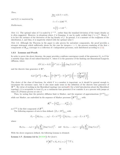
Then,<br />
and h (l) is maximized by<br />
Furthermore,<br />
lim a (d, l) = a (l) ,<br />
d→∞<br />
l = ˆl = 2.38I − 1 2 .<br />
)<br />
h<br />
(ˆl = 1.3I −1 .<br />
Note 1.5. The optimal value of l is s<strong>ca</strong>led by I −1/2 , rather than the standard deviation of the target density as<br />
is often suggested. However, in situations where f is Gaussian, it <strong>ca</strong>n be easily verified that I ≡ σ −2<br />
f<br />
. Hence, I<br />
is in fact the variance of the derivative of the log density of f. In general, I is a measure of the roughness of the<br />
distribution f, and thus, it is negatively related with the optimal value ˆl.<br />
Note 1.6. Although the Theorem in the paper is only proven for univariate components, the proof provides a<br />
stronger statement which sufficiently shows for the <strong>ca</strong>se for integers c > 1, the process consisting of the first c<br />
components of X [dt] converges to a collection of c independent processes, each distributed according to (1.2).<br />
1.3.5 Lemmas and Proofs<br />
In order to prove the above theorem, the paper provides a uniform convergence result of the generator G n to G for<br />
a suitably large class of real valued functions V , where G is the generator of the limiting one-dimensional Langevin<br />
diffusion, where<br />
and the discrete time generator of X n ,<br />
G d V<br />
[ 1<br />
GV (x) = h (l)<br />
2 V ′′ (x) + 1 2<br />
d<br />
dx (log f) (x) V ′ (x)<br />
⎡<br />
(<br />
x (d)) = dE Y (d)<br />
⎣ ( (<br />
V Y (d)) (<br />
⎛ ⎞⎤<br />
− V x (d))) π<br />
⎝1 ∧<br />
π ( x (d)) ⎠⎦ .<br />
]<br />
,<br />
(Y (d))<br />
The choice of the class of functions, for which V is a member is important, as it should be general enough to<br />
encompass the necessary <strong>ca</strong>ses, but it also must make sense in the definition of the discrete time generator of<br />
X (d) . By virtue of working in the Skorokhod topology (see sectionB.2 for a brief introduction about the Skorokhod<br />
topology), it is acceptable to treat G d as a continuous time generator if we consider it as a process with jumps at<br />
times of a Poisson process at rate d.<br />
Then, by noting that the putative diffusion limit is Markov, and the sequence of approximations { U (d)}<br />
{<br />
, d≥1<br />
while not Markov, are embedded in the sequence of Markov processes Z (d)} with<br />
d≥1,<br />
(<br />
)<br />
Z (d)<br />
t = X (d)<br />
[dt],1 , . . . , X(d) [dt] , d ,<br />
so U (d) is the first component of Z (d) .<br />
The following sequence of sets is then defined: { F d ⊂ R d} d>1 with<br />
where<br />
F d =<br />
R d (x 2 , . . . , x d ) = 1<br />
d − 1<br />
{<br />
} {<br />
}<br />
|R d (x 2 , . . . , x d ) − I| < d − 1 8 ∩ |S d (x 2 , . . . , x d ) − I| < d − 1 8 ,<br />
d∑<br />
i=2<br />
[<br />
(log f (xi )) ′] 2<br />
, and Sd (x 2 , . . . , x d ) = − 1<br />
d − 1<br />
With the above sequences defined, the following Lemma is obtained.<br />
Lemma 1.7. (Lemma 2.2 in [RGG97]) For fixed t,<br />
[<br />
P Z s<br />
(d) ∈ F d , 0 ≤ s ≤ t<br />
] d→∞<br />
−→ 1.<br />
d∑ [<br />
(log f (xi )) ′′] .<br />
i=2<br />
10


