final report - probability.ca

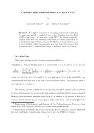
2.5 Optimal Scaling of RWM with Discontinuous Target Densities
2.5.1 Inefficiencies of full-dimensional updates using RWM applied to discontinuous targets
All the results proven thus far have been for continuous target densities. In [NRY05], the authors provide a weak
convergence result for a high-dimensional RWM algorithm applied to a target distribution which has a discontinuous
probability density function. In particular, they show that when the proposal variance is scaled by d −2 , the sequence
of stochastic processes formed by the first component of each Markov chain converges to a Langevin diffusion process
whose speed measure is optimized when the algorithm is tuned to yield an acceptance rate of e −2 ≈ 0.1353. Hence,
the mixing time for the RWM algorithm when applied to discontinuous densities is O ( d 2) . This work serves as a
validation of the result of [NR05], where it was found that lower dimensional updates are more efficient in the RWM
setting due to the lower computational cost. In fact, [NR05] showed that the Metropolis-within-Gibbs algorithms
mix with rate O (d), which compares favorably to the mixing rate of O ( d 2) required in the current context for
RWM algorithms applied to discontinuous target densities.
The target density in consideration is given by
where
( )
π x (d) , d =
d∏
f (x i ) ,
i=1
f (x) ∝ exp (g (x)) ,
with 0 < x < 1, g (·) twice differentiable on [0, 1], and f (x) = 0 otherwise.
2.5.2 Algorithm and Main Results
For d ≥ 1, consider a RWM algorithm on the d-dimensional hypercube with target density π ( x (d) , d ) as given
above. As always, suppose the algorithm starts in stationarity, so X (d)
0 ∼ π (·), and for t ≥ 0 and i ≥ 1, denote by
Z t,i elements of a sequence of i.i.d. uniform random variables with Z ∼ U [−1, 1] , with Z (d)
t = (Z t,1 , Z t,2 , . . . , Z t,d ).
For d ≥ 1, t ≥ 0 and l > 0, consider the proposals given by
Y (d)
t+1 = X(d) t + σ (d) Z (d)
t ,
(Y
(1, π (d)
where σ (d) = l/d. Accept these proposals with probability min
(
π
)
t+1
)
X (d)
t
{
( )
h z (d) 2 −d , z (d) ∈ (−1, 1) d
, d =
0, otherwise.
)
. Thus, for d ≥ 1, let
Given the current state of the process x (d) , denote by J ( x (d) , d ) the probability of accepting a proposal,
J
( ) ˆ
x (d) , d =
(
h z (d) , d) { min
(1, π ( x (d) + σ ( z (d) , d )) )}
π ( x (d)) dz (d) .
It is now necessary to define a pseudo-RWM process, which is identical to the regular RWM process except that it
(d) (d)
moves at every iteration. For d ≥ 1, let ˆX 0 , ˆX 1 , . . . denote the successive states of the pseudo-RWM process,
with
ˆX
(d)
given that
0 ∼ π (·). The pseudo-RWM process is a Markov process, where for t ≥ 0
ˆX
(d)
t
with z (d) ∈ R d .
= x (d) , the pdf of Ẑ(d) t
is given by
(
ζ z (d) |x (d)) ( )
= h z (d) , d min
{1, π ( x (d) + σ (d) z (d))
} /
π ( x (d)) J
ˆX
(d)
t+1 =
( )
x (d) , d ,
ˆX
(d)
t
+ σ (d) Ẑ(d) t , and
26