FIRE DESIGN OF STEEL MEMBERS - Civil and Natural Resources ...
FIRE DESIGN OF STEEL MEMBERS - Civil and Natural Resources ...
FIRE DESIGN OF STEEL MEMBERS - Civil and Natural Resources ...

You also want an ePaper? Increase the reach of your titles
YUMPU automatically turns print PDFs into web optimized ePapers that Google loves.
Fire Design of Steel Members<br />
K R Lewis<br />
Fire Engineering Research Report 2000/07<br />
March 2000<br />
ISSN 1173-5996
<strong>FIRE</strong> <strong>DESIGN</strong> <strong>OF</strong> <strong>STEEL</strong> <strong>MEMBERS</strong><br />
A report submitted in partial fulfilment of the<br />
requirements for the degree of<br />
Master of Fire Engineering<br />
at the<br />
University of Canterbury,<br />
Christchurch, New Zeal<strong>and</strong>.<br />
By Kathryn R. Lewis<br />
Supervised by Assoc. Prof. Andrew H. Buchanan<br />
February 2000
ABSTRACT:<br />
The New Zeal<strong>and</strong> Steel Code consists of few practical design tools other than finding<br />
the time <strong>and</strong> temperature that a simply supported steel member will fail. Many other<br />
design methods that consistently give accurate estimations of the behaviour of steel<br />
members have been published, <strong>and</strong> computer programmes developed to assist in the<br />
prediction of the temperature rise of steel when subjected to elevated temperatures<br />
environments.<br />
This report describes the origins of the fire design methods used in the New Zeal<strong>and</strong><br />
Steel Code, NZS 3404:1997. The New Zeal<strong>and</strong> Steel Code is reviewed <strong>and</strong> the design<br />
features are compared with the equivalent method found in the Eurocode, ENV 1993-<br />
1-2, which is the most advanced international steel fire code.<br />
The methods of evaluating the temperature rise of protected <strong>and</strong> unprotected steel<br />
beams are also investigated. Results from the simple formulas included in the New<br />
Zeal<strong>and</strong> Code, <strong>and</strong> those developed by the European Convention for Constructional<br />
Steelwork, ECCS, are compared with results from the time step ‘spreadsheet’ method<br />
<strong>and</strong> from the finite element computer programme, SAFIR, for the ISO 834 st<strong>and</strong>ard<br />
fire. The comparisons show that the spreadsheet method gives temperatures very close<br />
to the average temperatures calculated by SAFIR for all cross sections <strong>and</strong> protection<br />
layouts. The equations from ECCS <strong>and</strong> NZS 3404 give good results for unprotected<br />
steel, <strong>and</strong> for protected steel the ECCS equations appear to represent the thermal<br />
response of the steel quite accurately while the New Zeal<strong>and</strong> Steel Code has no simple<br />
method of estimating the temperatures for protected steel.<br />
The methods used for comparing the results with the ISO fire are then repeated with<br />
Eurocode Parametric fires, <strong>and</strong> with results from a real fire test.<br />
Suggested improvements are made for the New Zeal<strong>and</strong> Steel Code, to improve the<br />
concepts <strong>and</strong> information available to engineers designing for fire safety.<br />
i
ACKNOWLEDGMENTS:<br />
Throughout my time at university <strong>and</strong> throughout the course of this project I have<br />
received support <strong>and</strong> assistance from many people. I would especially like to thank<br />
the following:<br />
My supervisor, Associate Professor Andy Buchanan, thank you for the weekly<br />
meetings that kept me on track with this report, <strong>and</strong> your much needed input into this<br />
project.<br />
The Fire Service Commission, for the financial assistance you provided this year.<br />
All my friends who have helped me get through the workload of engineering school,<br />
<strong>and</strong> helped me enjoy my time away from this place, especially Alex, Andy, Jane, Julia,<br />
Lisa, <strong>and</strong> Ata for support over the last few weeks.<br />
The other postgrads on the third floor, the MEFE class <strong>and</strong> particularly Danza for<br />
providing me with entertainment throughout the year.<br />
My very supportive big sisters, who keep me well fed <strong>and</strong> well dressed.<br />
And lastly but mostly, my parents, for their never ending encouragement <strong>and</strong> faith that<br />
I would get there in the end, when I have doubted myself over the past five years.<br />
iii
TABLE <strong>OF</strong> CONTENTS:<br />
ABSTRACT:.............................................................................................................................. I<br />
ACKNOWLEDGMENTS: .................................................................................................... III<br />
LIST <strong>OF</strong> FIGURES: ...............................................................................................................IX<br />
1 INTRODUCTION:...........................................................................................................1<br />
1.1 OBJECTIVES:...................................................................................................................1<br />
1.2 PREVIOUS STUDIES:........................................................................................................1<br />
1.3 SCOPE <strong>OF</strong> THIS REPORT: ..................................................................................................6<br />
1.4 NZS 3404:PART 1:1997 SECTION 11:............................................................................7<br />
1.5 OTHER <strong>STEEL</strong> CODES .....................................................................................................8<br />
1.5.1 BS 5950:Part 8:1990.............................................................................................8<br />
1.5.2 AS 4100:1990 ........................................................................................................9<br />
1.5.3 ENV 1993-1-2........................................................................................................9<br />
1.6 BACKGROUND INFORMATION:......................................................................................10<br />
1.6.1 Forms of Heat Transfer:......................................................................................10<br />
1.6.2 Thermal Properties of Steel:................................................................................11<br />
1.6.3 Section Factor, H p /A:...........................................................................................15<br />
1.6.4 Methods of steel protection: ................................................................................17<br />
2 <strong>FIRE</strong>S AND THERMAL ANALYSIS COMPUTER MODELS: ..............................19<br />
2.1 SPREADSHEET METHOD: ..............................................................................................19<br />
2.1.1 Introduction:........................................................................................................19<br />
2.1.2 Unprotected Steel: ...............................................................................................20<br />
2.1.3 Protected steel:....................................................................................................21<br />
2.2 ALTERNATIVE FORMULATIONS <strong>OF</strong> THE SPREADSHEET METHOD: ................................23<br />
2.3 THERMAL ANALYSIS PROGRAMMES:...........................................................................26<br />
2.3.1 SAFIR: .................................................................................................................26<br />
2.3.2 Firecalc: ..............................................................................................................28<br />
2.4 <strong>FIRE</strong> CURVES: ...............................................................................................................30<br />
2.4.1 St<strong>and</strong>ard Fire – ISO 834: ....................................................................................30<br />
2.4.2 Eurocode Parametric fire:...................................................................................31<br />
3 <strong>FIRE</strong> SECTION <strong>OF</strong> THE <strong>STEEL</strong> CODES:................................................................35<br />
3.1 NZS3404/AS4100:.......................................................................................................35<br />
v
3.1.1 Determination of Period of Structural Adequacy (PSA): ....................................35<br />
3.1.2 Variation of Mechanical Properties of Steel with Temperature:.........................36<br />
3.1.3 Determination of Limiting Steel Temperature:....................................................42<br />
3.1.4 Temperature rise of unprotected steel: ................................................................43<br />
3.1.5 Temperature rise of protected steel: ....................................................................44<br />
3.1.6 Determination of PSA from a single test: ............................................................46<br />
3.1.7 Special Considerations:.......................................................................................47<br />
4 CALCULATION <strong>OF</strong> <strong>STEEL</strong> TEMPERATURES FOR UNPROTECTED <strong>STEEL</strong> –<br />
ISO <strong>FIRE</strong>: ................................................................................................................................51<br />
4.1 INTRODUCTION: ............................................................................................................51<br />
4.1.1 Assumptions .........................................................................................................52<br />
4.1.2 Analysis Between Methods of Temperature Evaluation: .....................................53<br />
4.2 RESULTS FOR FOUR SIDED EXPOSURE: ........................................................................54<br />
Results from a simulation with the SAFIR programme: ...................................................54<br />
4.2.2 Unprotected steel beam with four sided exposure:..............................................57<br />
4.2.3 Comparison with NZS 3404 <strong>and</strong> ECCS formulas for four sided exposure:.........59<br />
4.3 RESULTS FOR THREE SIDED EXPOSURE:.......................................................................63<br />
4.3.1 Results from simulations with the SAFIR programme:........................................65<br />
4.3.2 Unprotected steel beam with three sided exposure: ............................................68<br />
4.3.3 Comparison with NZS 3404 <strong>and</strong> ECCS formulas for three sided exposure: .......71<br />
4.4 COMPARISONS WITH OTHER FINITE ELEMENT PROGRAMMES:....................................75<br />
4.4.1 Comparison of <strong>FIRE</strong>S-T2 with SAFIR:................................................................75<br />
4.4.2 Comparison with Firecalc:..................................................................................77<br />
4.5 CONCLUSIONS:..............................................................................................................78<br />
5 CALCULATION <strong>OF</strong> <strong>STEEL</strong> TEMPERATURES FOR PROTECTED <strong>STEEL</strong> –<br />
ISO <strong>FIRE</strong>: ................................................................................................................................81<br />
5.1 INTRODUCTION: ............................................................................................................81<br />
5.1.1 Assumptions:........................................................................................................81<br />
5.2 RESULTS FOR FOUR SIDED EXPOSURE WITH HEAVY PROTECTION:.............................82<br />
5.2.1 Results from a simulation with the SAFIR programme: ......................................83<br />
5.2.2 Heavily Protected Beam with Four Sided Exposure: ..........................................85<br />
5.2.3 Comparison with the ECCS equation:.................................................................88<br />
5.3 RESULTS FOR FOUR SIDED EXPOSURE WITH LIGHT PROTECTION:................................91<br />
5.3.1 Lightly Protected Beams with Four Sided Exposure:..........................................92<br />
5.3.2 Comparison with the ECCS Formula:.................................................................97<br />
vi
5.4 RESULTS FOR FOUR SIDED EXPOSURE WITH BOX PROTECTION:...................................99<br />
5.4.1 Steel Beams with Box Protection:......................................................................100<br />
5.5 RESULTS FOR FOUR SIDED EXPOSURE WITH THICK PROTECTION: ..............................102<br />
5.5.1 Results from a Simulation in the SAFIR programme: .......................................103<br />
5.5.2 Comparison with the ECCS equation:...............................................................104<br />
5.6 RESULTS FOR THREE SIDED EXPOSURE WITH HEAVY PROTECTION:...........................106<br />
5.6.1 Results from a Simulation with the SAFIR Programme: ...................................107<br />
5.6.2 Heavily Protected Beams with Three Sided Exposure: .....................................109<br />
5.6.3 Comparison with the ECCS Formula:...............................................................111<br />
5.7 COMPARISONS WITH <strong>FIRE</strong>CALC:.................................................................................113<br />
5.7.1 Heavily Protected Beam with Three Sided Exposure:.......................................113<br />
5.8 CONCLUSIONS: ...........................................................................................................115<br />
6 COMPARISON <strong>OF</strong> METHODS USING OTHER <strong>FIRE</strong> CURVES: ......................117<br />
6.1 INTRODUCTION:..........................................................................................................117<br />
6.2 EUROCODE PARAMETRIC <strong>FIRE</strong>S: ................................................................................117<br />
6.2.1 Introduction:......................................................................................................117<br />
6.2.2 Assumptions:......................................................................................................118<br />
6.2.3 Results for unprotected steel exposed to the Eurocode Parametric fire: ..........118<br />
6.2.4 Results for protected steel: ................................................................................121<br />
6.3 REAL <strong>FIRE</strong>S:................................................................................................................123<br />
6.3.1 Unprotected Steel: .............................................................................................124<br />
6.3.2 Protected Steel:..................................................................................................126<br />
7 ADDITIONAL MATERIAL IN EUROCODE 3:......................................................129<br />
7.1 INTRODUCTION:..........................................................................................................129<br />
7.2 ANALYSIS <strong>OF</strong> THE EUROCODE:...................................................................................130<br />
7.2.1 Design Methods for Performance Requirements: .............................................130<br />
7.2.2 Structural fire Design:.......................................................................................132<br />
7.2.3 Thermal Analysis of Steel Members: .................................................................136<br />
7.2.4 Mechanical Properties: .....................................................................................137<br />
7.2.5 Thermal Properties: ..........................................................................................138<br />
7.2.6 External Steelwork: ...........................................................................................139<br />
8 CONCLUSIONS AND RECOMMENDATIONS: ....................................................143<br />
8.1 UNPROTECTED <strong>STEEL</strong> <strong>MEMBERS</strong>: ..............................................................................143<br />
8.2 PROTECTED <strong>STEEL</strong> <strong>MEMBERS</strong>: ...................................................................................143<br />
8.3 CHANGES TO NZS 3404: ............................................................................................144<br />
vii
8.4 FURTHER RESEARCH: .................................................................................................144<br />
9 NOMENCLATURE: ....................................................................................................145<br />
10 REFERENCES: ............................................................................................................147<br />
APPENDIX A – SPREADSHEET METHOD:...................................................................153<br />
APPENDIX B – SAFIR:........................................................................................................155<br />
SAFIR INPUT.........................................................................................................................156<br />
DIAMOND OUTPUT...............................................................................................................160<br />
APPENDIX C – <strong>FIRE</strong>CALC................................................................................................161<br />
viii
LIST <strong>OF</strong> FIGURES:<br />
FIGURE 1.1: VARIATION <strong>OF</strong> THE SPECIFIC HEAT <strong>OF</strong> <strong>STEEL</strong> WITH TEMPERATURE. .....................13<br />
FIGURE 1.2:VARIATION <strong>OF</strong> THERMAL CONDUCTIVITY <strong>OF</strong> <strong>STEEL</strong> WITH TEMPERATURE.............14<br />
FIGURE 1.3: VARIATION <strong>OF</strong> THERMAL EXPANSION <strong>OF</strong> <strong>STEEL</strong> WITH TEMPERATURE..................15<br />
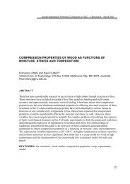
FIGURE 1.4: VARIATIONS <strong>OF</strong> HP/A FOR DIFFERENT METHODS <strong>OF</strong> PROTECTION .......................16<br />
FIGURE 2.1: SPREADSHEET CALCULATION FOR HEAT TRANSFER IN UNPROTECTED <strong>STEEL</strong><br />
<strong>MEMBERS</strong> ..........................................................................................................................20<br />
FIGURE 2.2: COMPARISON BETWEEN THE ECCS FORMULA, EQUATION 2.6, AND THE<br />
SPREADSHEET METHOD FOR HEAVY INSULATION.............................................................24<br />
FIGURE 2.3: COMPARISON BETWEEN THE EC3 FORMULA, EQUATION 2.8, AND THE<br />
SPREADSHEET METHOD.....................................................................................................25<br />
FIGURE 2.4: TIME TEMPERATURE CURVE <strong>OF</strong> THE ISO 834 STANDARD <strong>FIRE</strong> CURVE................30<br />
FIGURE 2.5: EUROCODE <strong>FIRE</strong>S WITH VARYING VENTILATION FACTORS AND FUEL LOADS.......32<br />
FIGURE 3.1: VARIATION <strong>OF</strong> THE MODULUS <strong>OF</strong> ELASTICITY WITH TEMPERATURE ...................37<br />
FIGURE 3.2: VARIATION <strong>OF</strong> THE YIELD STRESS <strong>OF</strong> <strong>STEEL</strong> WITH TEMPERATURE........................38<br />
FIGURE 3.3: VARIATION <strong>OF</strong> YIELD STRESS AND MODULUS <strong>OF</strong> ELASTICITY WITH<br />
TEMPERATURE ..................................................................................................................39<br />
FIGURE 3.4: STRESS STRAIN CURVES WITH VARYING TEMPERATURE.......................................41<br />
FIGURE 3.5: VARIATION <strong>OF</strong> ULTIMATE AND YIELD STRENGTH <strong>OF</strong> HOT ROLLED <strong>STEEL</strong>.............41<br />
FIGURE 4.1: SCHEMATIC GRAPH SHOWING THE COMPARISONS MADE BETWEEN APPROXIMATE<br />
FORMULAS AND TIME TEMPERATURE CURVES .................................................................53<br />
FIGURE 4.2: TIME TEMPERATURE CURVE FROM A SAFIR SIMULATION SHOWING THE<br />
VARIATION <strong>OF</strong> TEMPERATURE FOR FOUR SIDED EXPOSURE..............................................54<br />
FIGURE 4.3: TEMPERATURE CONTOUR LINES SHOWING THE TEMPERATURE PR<strong>OF</strong>ILE OVER THE<br />
CROSS SECTION <strong>OF</strong> THE <strong>STEEL</strong> SECTION............................................................................57<br />
FIGURES 4.4 A-C: COMPARISON BETWEEN THE RESULTS FROM SAFIR AND THE SPREADSHEET<br />
METHOD FOR UNPROTECTED <strong>STEEL</strong> BEAMS WITH FOUR SIDED EXPOSURE ......................58<br />
FIGURE 4.5 A-C: COMPARISON <strong>OF</strong> THE LINEAR EQUATIONS PROVIDED BY NZS 3404 AND ECCS<br />
WITH THE TEMPERATURES OBTAINED FROM THE SPREADSHEET METHOD WITH FOUR<br />
SIDED EXPOSURE TO AN ISO 834 <strong>FIRE</strong>..............................................................................61<br />
FIGURE 4.6: LAYOUT <strong>OF</strong> THREE SIDED EXPOSURE WITH A CONCRETE SLAB.............................64<br />
FIGURE 4.7: MAXIMUM, AVERAGE AND MINIMUM TEMPERATURES FOUND FROM THE SAFIR 1<br />
SIMULATION......................................................................................................................65<br />
FIGURE 4.8: MAXIMUM, AVERAGE AND MINIMUM TEMPERATURES FOUND FROM THE SAFIR 2<br />
SIMULATION......................................................................................................................65<br />
ix
FIGURE 4.9: LOCATION <strong>OF</strong> MAXIMUM AND MINIMUM <strong>STEEL</strong> TEMPERATURES ON THE CROSS<br />
SECTION <strong>OF</strong> A BEAM FOR THREE SIDED EXPOSURE............................................................66<br />
FIGURE 4.10: MAXIMUM TEMPERATURES FROM SIMULATIONS IN SAFIR <strong>OF</strong> FOUR SIDED<br />
EXPOSURE, AND THREE SIDED WITH AND WITHOUT A SLAB. ............................................68<br />
FIGURE 4.11A-C: COMPARISON <strong>OF</strong> RESULTS FROM SAFIR AND THE SPREADSHEET METHOD<br />
FOR AN UNPROTECTED <strong>STEEL</strong> MEMBER SUBJECTED TO THREE SIDED EXPOSURE .............69<br />
FIGURE 4.12 A-C: COMPARISON <strong>OF</strong> THE LINEAR EQUATIONS PROVIDED BY NZS 3404 AND<br />
ECCS WITH SAFIR WITH THREE SIDED EXPOSURE TO AN ISO 834 <strong>FIRE</strong>.........................73<br />
FIGURE 4.14: COMPARISON BETWEEN THE RESULTS FROM THE SAFIR PROGRAMME WITH<br />
TEMPERATURE RESULTS FROM <strong>FIRE</strong>S-T2 ........................................................................75<br />
FIGURE 4.15: COMPARISON BETWEEN THE SPREADSHEET METHOD, SAFIR AND <strong>FIRE</strong>CALC FOR<br />
AN UNPROTECTED BEAM EXPOSED ON THREE SIDES TO ISO 834 <strong>FIRE</strong>..............................77<br />
FIGURE 5.1: TIME TEMPERATURE CURVE FROM A SAFIR SIMULATION FOR FOUR SIDED<br />
EXPOSURE TO AN ISO <strong>FIRE</strong>................................................................................................83<br />
FIGURE 5.2: LOCATION <strong>OF</strong> THE MAXIMUM AND MINIMUM TEMPERATURES ON THE CROSS<br />
SECTION <strong>OF</strong> A <strong>STEEL</strong> BEAM WITH SPRAY ON PROTECTION ................................................84<br />
FIGURE 5.3 A-C: COMPARISON BETWEEN THE RESULTS FROM SAFIR AND THE SPREADSHEET<br />
METHOD FOR FENDOLITE PROTECTED <strong>STEEL</strong> BEAMS WITH FOUR SIDED EXPOSURE TO THE<br />
ISO STANDARD <strong>FIRE</strong>. ........................................................................................................86<br />
FIGURE 5.4 A-C: COMPARISON <strong>OF</strong> THE LINEAR EQUATIONS PROVIDED BY NZS 3404 AND ECCS<br />
WITH THE TEMPERATURES OBTAINED FROM THE SPREADSHEET METHOD WITH FOUR<br />
SIDED EXPOSURE TO AN ISO 834 <strong>FIRE</strong>. .............................................................................90<br />
FIGURE 5.5 A-C: COMPARISON BETWEEN THE RESULTS FROM SAFIR WITH THE SIMPLIFIED<br />
AND FULL SPREADSHEET METHODS FOR A BEAM WITH LIGHT INSULATE PROTECTION. ...94<br />
FIGURE 5.6: COMPARISON BETWEEN SAFIR AND THE SPREADSHEET METHOD WITH VARYING<br />
THERMAL PROPERTIES.......................................................................................................96<br />
FIGURE 5.7 A-C: COMPARISON BETWEEN THE RESULTS FROM THE TWO SPREADSHEET<br />
METHODS, SAFIR AND THE ECCS RECOMMENDED FORMULA FOR <strong>STEEL</strong> WITH LIGHT<br />
INSULATION PROTECTION..................................................................................................98<br />
FIGURE 5.8 A-C: COMPARISON BETWEEN THE RESULTS FROM THE SPREADSHEET METHOD AND<br />
SAFIR FOR PROTECTED <strong>STEEL</strong> BEAMS WITH 20 MM BOARD PROTECTION .....................101<br />
FIGURE 5.9: MAXIMUM, AVERAGE AND MINIMUM TEMPERATURES FOUND FROM A SAFIR<br />
SIMULATION WITH 40 MM HEAVY PROTECTION..............................................................103<br />
FIGURE 5.10 A-C: COMPARISON BETWEEN RESULTS FROM THE SPREADSHEET METHOD WITH<br />
THE RESULTS FROM SAFIR AND WITH THE ECCS EQUATIONS FOR PROTECTED <strong>STEEL</strong><br />
<strong>MEMBERS</strong> WITH HEAVY THICK PROTECTION. ..................................................................105<br />
x
FIGURE 5.11: TEMPERATURE CONTOUR LINES FOR A BEAM PROTECTED WITH FENDOLITE AND<br />
WITH A 20 MM CONCRETE SLAB, EXPOSED TO THE ISO 834 <strong>FIRE</strong> ..................................108<br />
FIGURE 5.12: VARIATION <strong>OF</strong> MAXIMUM AND MINIMUM TEMPERATURES FROM A SIMULATION<br />
IN SAFIR FOR A BEAM WITH HEAVY PROTECTION AND CONCRETE SLAB. .....................109<br />
FIGURE 5.13: COMPARISON BETWEEN TEMPERATURES FROM SAFIR WITH THE SPREADSHEET<br />
CALCULATIONS FOR A BEAM EXPOSED TO AN ISO <strong>FIRE</strong> ON THREE SIDES. .....................110<br />
FIGURE 5.14: COMPARISON BETWEEN THE RESULTS FROM SAFIR AND THE SPREADSHEET<br />
METHOD WITH THE ECCS EQUATION FOR PROTECTED <strong>STEEL</strong> <strong>MEMBERS</strong> WITH THREE<br />
SIDED EXPOSURE TO THE ISO 834 <strong>FIRE</strong>. .........................................................................112<br />
FIGURE 5.15: COMPARISON BETWEEN RESULTS FROM <strong>FIRE</strong>CALC, SAFIR AND THE<br />
SPREADSHEET METHOD FOR A BEAM WITH 20 MM HEAVY PROTECTION........................114<br />
FIGURE 6.1 A-C: COMPARISON BETWEEN SAFIR AND SPREADSHEET RESULTS FOR AN<br />
UNPROTECTED <strong>STEEL</strong> BEAM WITH FOUR SIDED EXPOSURE TO A PARAMETRIC <strong>FIRE</strong>.......119<br />
FIGURES 6.2 A-B: COMPARISON BETWEEN THE RESULTS FROM SAFIR AND THE SPREADSHEET<br />
METHOD FOR PROTECTED <strong>STEEL</strong> EXPOSED TO A EUROCODE PARAMETRIC <strong>FIRE</strong> ............121<br />
FIGURE 6.3: COMPARISON BETWEEN TEMPERATURE FROM EXPERIMENTAL DATA FOR THREE<br />
SIDED UNPROTECTED <strong>STEEL</strong> WITH THE SPREADSHEET METHOD AND SAFIR.................124<br />
FIGURE 6.4: COMPARISON BETWEEN RESULTS FROM AN EXPERIMENTAL <strong>FIRE</strong> TEST WITH THE<br />
TEMPERATURES FROM SAFIR, AND FROM THE SPREADSHEET METHOD........................125<br />
FIGURE 6.5: COMPARISON BETWEEN RESULTS FROM AN EXPERIMENTAL <strong>FIRE</strong> TEST WITH THE<br />
TEMPERATURES FROM SAFIR, AND FROM THE SPREADSHEET METHOD FOR PROTECTED<br />
<strong>STEEL</strong>. .............................................................................................................................127<br />
FIGURE A.1: EXAMPLE <strong>OF</strong> THE SPREADSHEET METHOD FOR AN UNPROTECTED BEAM. .........153<br />
FIGURE A.2: EXAMPLE <strong>OF</strong> THE SPREADSHEET METHOD FOR A PROTECTED BEAM. ...............154<br />
FIGURE B.1: WINDOW DEVELOPED BY JOHN MASON AS A PREPROCESSOR FOR THE SAFIR<br />
PROGRAMME. ..................................................................................................................155<br />
FIGURE B.2: OUTPUT WINDOW <strong>OF</strong> THE DIAMOND PROGRAMME.............................................160<br />
FIGURE C.1: WINDOW FORMAT FOR <strong>FIRE</strong>CALC.......................................................................161<br />
xi
1 INTRODUCTION:<br />
1.1 OBJECTIVES:<br />
The objectives of this study are:<br />
1. To outline the design methods for fire engineering that are included in the fire<br />
section of the New Zeal<strong>and</strong> Steel Code, NZS 3404:1997, determine their origin,<br />
<strong>and</strong> make comparisons of these with other equivalent codes from around the world.<br />
2. To examine the validity <strong>and</strong> assumptions of the formulas given in the New Zeal<strong>and</strong><br />
Steel Code, <strong>and</strong> other international Steel Codes by comparing the formulas with<br />
simulations from computer programmes. The results from these methods will then<br />
be compared with results from tests completed on steel members where appropriate<br />
<strong>and</strong> available.<br />
3. To make recommendations based on the results of this project, for changes to the<br />
New Zeal<strong>and</strong> Steel Code, or alternatively to confirm the existing methods where<br />
appropriate.<br />
1.2 PREVIOUS STUDIES:<br />
Many other studies have been performed comparing the results from different methods<br />
of evaluating the temperature of steel members in elevated temperature environments.<br />
The purpose of these studies has varied from whether to establish a clear comparison<br />
of time equivalence methods; to comparing the different methods for cost saving<br />
reasons; or to further increase the confidence that designers have in the tools that are<br />
available to them.<br />
Performance based design uses fire engineering principles to estimate <strong>and</strong> evaluate a<br />
structure’s behaviour in a realistic design fire. The design is replacing prescriptive<br />
code in which the design of members is based on the results of tests that may not<br />
necessarily be relevant or appropriate to use for the structure being considered.<br />
With the increase in performance based design being utilised around the world, there is<br />
a requirement for accurate estimations of member behaviour in fire so designs can be<br />
1
designed with confidence. Full scale tests are expensive, time consuming <strong>and</strong> can only<br />
be performed on a limited number of structural elements. Computer programmes <strong>and</strong><br />
simple formulas, however, can be easily modified by changing a value applicable to<br />
the case, <strong>and</strong> once complicated methods are established, they can be reused by entering<br />
the appropriate information for the case.<br />
Feeney, (1998), examined the design of a multistorey steel framed building without<br />
applying protective coatings, using performance based design. This report gives a<br />
background on the loadings for a building from a structural perspective <strong>and</strong> treats the<br />
fire loading in a similar way. The structure needs to be able to support a dead <strong>and</strong> live<br />
load under normal conditions <strong>and</strong> although the strength of the element decreases with<br />
increased temperature, so does the loading enforced on the element.<br />
A detailed description is given to determine the maximum steel temperatures reached<br />
during a fire based on the ISO fire <strong>and</strong> a ‘real’ fire as determined from the Annex to<br />
Eurocode 1. An evaluation of structural performance is made based on the effects of<br />
increased temperature on the steel strength, load sharing between members of the<br />
structure <strong>and</strong> the design load likely to be present during a fire. A case study design of<br />
an apartment building in Auckl<strong>and</strong> is worked through with the loads <strong>and</strong> temperatures<br />
estimated during a fire <strong>and</strong> the expected resulting strength calculated. A hotel building<br />
in Auckl<strong>and</strong> is also similarly examined. This article shows that performance based<br />
design can eliminate the requirements of passive protection, reducing the cost of the<br />
building.<br />
The suggestion in his report is to design for fire conditions so that protection is not<br />
required because the fire resistance of the unprotected steel member is sufficient in a<br />
fire. The conclusions however find the maximum likely temperature of the steel to be<br />
within 2 °C of the limiting temperature which is not very supportive evidence given<br />
the assumptions made <strong>and</strong> variability of steel beam sizes <strong>and</strong> properties when in place.<br />
Spearpoint, (1998), compared the results from a finite element computer programme,<br />
THELMA, with results from a full size fire test at the test facility at Cardington, UK.<br />
The results showed THELMA gave reasonable predictions of the temperature profiles<br />
for unprotected steel members, but for protected steel the predictions did not compare<br />
2
as well with the experimental data. Results were compared for beams <strong>and</strong> columns<br />
between the results found from THELMA <strong>and</strong> the experimental data.<br />
Bennetts, Proe <strong>and</strong> Thomas wrote a series of articles in 1986 on the calculation of the<br />
response of structural elements, on the thermal response, mechanical response <strong>and</strong><br />
overall behaviour. The report (Bennett et al, 1986) on the thermal response includes<br />
an introduction giving background to the regulations of the existing codes at the time<br />
of when written. It also has a procedure for calculating the overall behaviour of a<br />
structural element in a fire based on thermal response of the element <strong>and</strong> strength of<br />
the element as a function of temperature. Methods for calculating the thermal response<br />
for protected <strong>and</strong> unprotected steel members are given. Various methods for<br />
calculating behaviour of protected members are given including methods with or<br />
without moisture <strong>and</strong> the CTICM method. These methods use simplified heat flow<br />
theory to predict the behaviour of steel members Regression analyses were also<br />
performed in the report to provide estimates <strong>and</strong> confidence limits of the temperature<br />
of the steel member. An application of the test results is included also, which<br />
compares theoretical calculations with experimental results.<br />
Proe et al 1 , (1986) is the second article of the series <strong>and</strong> outlines the mechanical<br />
response of steel including a brief overview of the purpose of the fire test – for<br />
calculating the thermal response of an element under fire loading <strong>and</strong> the strength of<br />
the element as a function of temperature of the element. The relationship between the<br />
tests to ECCS recommendations is commented on. A review of plastic analysis<br />
behaviour of steel members is included <strong>and</strong> methods to apply the basic principles to<br />
simply supported beams, built in beams, multi-span beams <strong>and</strong> struts. Plastic analysis<br />
under fire conditions is looked at with an outline of the behaviour of steel under<br />
elevated temperatures. Variation of steel strength with temperature is covered, when<br />
the member is treated as an isothermal member, <strong>and</strong> when variation within a member<br />
either along the member or within the depth of the member is considered. Mechanical<br />
properties of steel in a member such as expansion, modulus of elasticity <strong>and</strong> strength<br />
of struts is looked at. An analysis of the fire test behaviour includes correlations<br />
between the theoretical calculations <strong>and</strong> experimental data for beams with uniform<br />
temperature distribution, beams with a concrete slab <strong>and</strong> struts at uniform<br />
temperature.This paper uses methods to determine the load capacities of isolated<br />
3
eams <strong>and</strong> struts when subjected to a fire test. The plastic analysis method presented<br />
here assesses the member capacity under normal conditions <strong>and</strong> this analysis is<br />
extended.<br />
Proe et al 2 (1986) is the third report which includes a summary of the thermal <strong>and</strong><br />
mechanical response reports in this series. It also has methods to calculate overall<br />
response of the member, for beams <strong>and</strong> columns at uniform temperature <strong>and</strong> with<br />
temperature gradients within the depth of the member or along the member. The test<br />
data is correlated to the calculated results for results that both thermal <strong>and</strong> mechanical<br />
response can be calculated for. This includes beams with uniform temperatures <strong>and</strong><br />
with temperature gradients <strong>and</strong> for columns with uniform temperature.<br />
Although these articles are now dated <strong>and</strong> a lot of the results found have been further<br />
researched <strong>and</strong> different results found, this series was used extensively in the writing<br />
of the present New Zeal<strong>and</strong> Steel Code.<br />
In Kodur et al, (1999), there is a brief background to the design of steel structures <strong>and</strong><br />
difference in performance based on analysing a single member compared with a<br />
complete structure. Background information about SAFIR is given <strong>and</strong> about the<br />
finite element method of analysis. The assumptions made when determining the<br />
element properties <strong>and</strong> magnitudes of displacements <strong>and</strong> rotation are included as is the<br />
procedure for analysis of the behaviour of a structure. A case study analysis of three<br />
members is worked through withfourdifferent fire protection options on the elements.<br />
An ISO 834 fire curve is used to model the fire <strong>and</strong> output was set to come out at 2<br />
minute increments, with the analysis continuing until failure occurs in one of the<br />
members. The results of the four tests are given with comparisons between them. The<br />
paper concludes that SAFIR can be used to perform thermal <strong>and</strong> structural analysis,<br />
<strong>and</strong> that SAFIR can be used to study the overall behaviour of structures under fire<br />
conditions because it is of finite element formulation.<br />
It also concludes that there is an improvement in the fire resistance performance of a<br />
beam when acting as a part of a structure than when acting alone as a single member,<br />
4
<strong>and</strong> that the effect of slab-beam interaction has to be accounted for in the analysis to<br />
assess the realistic fire resistance of a steel frame.<br />
Milke, (1999) describes the work that is being done by a joint ASCE <strong>and</strong> SFPE<br />
committee working towards a st<strong>and</strong>ard for performance based fire resistance analyses.<br />
This st<strong>and</strong>ard will include: descriptions of characteristics of exposure from a design<br />
fire; material properties at elevated temperatures <strong>and</strong> heat transfer <strong>and</strong> structural<br />
analysis methods. This paper therefore includes a background of the requirements that<br />
structural members must uphold during a fire. The fire exposure to the member needs<br />
to be characterised <strong>and</strong> the heat transfer coefficients <strong>and</strong> temperature needs to be<br />
specified for different scenarios. The properties of steel at elevated temperatures<br />
change from that of ambient conditions <strong>and</strong> this affects the thermal response, <strong>and</strong><br />
structural analysis. Included in this paper is an overview of the heat transfer <strong>and</strong><br />
structural analysis methods including moment analyses for beams <strong>and</strong> slabs <strong>and</strong><br />
stability analyses for columns <strong>and</strong> walls.<br />
Gamble, (1989) wrote an early paper giving the background <strong>and</strong> theory to the<br />
spreadsheet method of predicting the temperature of protected steel beams. The paper<br />
includes three worked examples with different types of protection <strong>and</strong> the response<br />
that the steel member should have, with all working to make a clear guide. The theory<br />
to the formation of the equations used is provided, as are explanations with examples.<br />
Franssen et al, (1994), wrote a report comparing 5 different computer programmes,<br />
analysing three structures under different temperature profiles, with 8 comparisons<br />
being made in total. The computer programmes examined are CEFICOSS, DIANA,<br />
LENAS, SAFIR <strong>and</strong> SISMEF. The horizontal displacement is given graphically for<br />
each test, <strong>and</strong> maximum values summarised in a table. The maximum difference in<br />
ultimate values between any two programmes was found to be 6%, although DIANA<br />
had a substantial deviation from the others for heating with an axially loaded column.<br />
Some explanations are offered for the difference between DIANA <strong>and</strong> the other<br />
programmes, but no firm conclusion as to the reason is given. The programmes are<br />
concluded to be very similar for bending members, <strong>and</strong> for members with axial loads,<br />
the ultimate loads can be found with some confidence, however the history of the<br />
member can not be accurately given.<br />
5
Gilvery <strong>and</strong> Dexter, (1997), prepared a report for <strong>and</strong> funded by NIST to determine the<br />
possibility of using a computer programme to estimate or evaluate fire resistance times<br />
<strong>and</strong> load capacity of structures subjective to fire, instead of conducting full scale<br />
furnace tests. The purpose behind the project was to establish if a computer could<br />
accurately model the behaviour of a member in a fire, <strong>and</strong> therefore save a lot of<br />
money. A range of possible approaches were evaluated from simple calculations to<br />
sophisticated numerical simulations. Simple calculations were found to be good for<br />
members with a uniform temperature distribution, but for members with non uniform<br />
temperature distributions, computer programmes were better. The paper reports that<br />
one of the best computer programmes is SAFIR in terms of its ‘user friendliness’ <strong>and</strong><br />
accuracy. The use of SAFIR is shown by modelling complex structural elements, <strong>and</strong><br />
evaluating special situations such as partial fire exposure <strong>and</strong> exposure of a continuous<br />
frame to fire in one bay. It is concluded that SAFIR is a very useful tool that could be<br />
used as an alternative to furnace testing.<br />
A University of Canterbury research report by Wong, (1999), on the reliability of<br />
Structural Fire Design used the computer package @RISK to calculate the probability<br />
of failure of structural steel elements designed for fire conditions. The @RISK<br />
programme uses the st<strong>and</strong>ard deviation of the factors involved in the design of a steel<br />
member <strong>and</strong> runs simulations to find the probability of failure of the member with all<br />
factors considered. The results show the shortcomings in design <strong>and</strong> an option to<br />
enhance the performance based design of structures.<br />
1.3 SCOPE <strong>OF</strong> THIS REPORT:<br />
This report is concerned with the design of single simply supported beams <strong>and</strong><br />
columns that will fail when the load capacity is reached <strong>and</strong> exceeded at one critical<br />
point of the span, when a plastic hinge will develop <strong>and</strong> cause failure of the steel<br />
member. The results found in this report do not apply to complex structural<br />
arrangements such as frames <strong>and</strong> built in members as the effects from moment<br />
distribution between individual members means that multiple plastic hinges must form<br />
before failure occurs.<br />
6
Results from experimental tests show that more complex structural arrangements often<br />
have more fire resistance than single members. Results from series of tests from<br />
Cardington <strong>and</strong> articles such as O’Connor <strong>and</strong> Martin, (1998) who reported the results<br />
of tests studied by British Steel indicate that unprotected steel frames behave<br />
significantly better than indicated in single member tests.<br />
1.4 NZS 3404:PART 1:1997 SECTION 11:<br />
The New Zeal<strong>and</strong> Steel code, (SNZ, 1997) includes a section devoted to the fire safety<br />
of essential steel elements of a structure. The section includes formulas to estimate the<br />
maximum temperature that an element can reach before it will no longer be able to<br />
carry the design fire load <strong>and</strong> therefore fail, <strong>and</strong> the time until this temperature is<br />
reached. These formulas are based on the member ends being simply supported, so no<br />
redistribution of loads is allowed for. This gives a conservative design of elements as<br />
a lower temperature of the element will result in failure than if the element was ‘built<br />
in’ to a frame with axial restraint <strong>and</strong> moment redistribution possible.<br />
Other design tools for fire included in the section are formulas that estimate the<br />
variation in mechanical properties of steel with temperature. These are the Yield<br />
Stress <strong>and</strong> Modulus of Elasticity of steel, whose variation with temperature dictates the<br />
strength of the steel at a particular temperature<br />
The time until the limiting temperature is reached, the variation of temperature across<br />
the cross section <strong>and</strong> the rate at which the temperature increases, depends on the<br />
element cross section, the perimeter exposed to the fire <strong>and</strong> the protection applied to<br />
the member. This is accounted for in the code equations by a ratio of the heated<br />
perimeter of the member to the cross sectional area of the steel member, known as the<br />
section factor, or H p /A (m -1 ). This value is the inverse of the average thickness of the<br />
steel member so gives an indication to the rate of temperature rise.<br />
In NZS 3404:1997, there are formulas provided for three <strong>and</strong> four sided exposure to<br />
the fire for unprotected members. For protected members the temperature of the<br />
element with time is based on a single experimental test exposed to a st<strong>and</strong>ard fire,<br />
7
with conditions specified to ensure that the results of the test will be equal or more<br />
conservative than what will occur in the element being examined.<br />
If results of a series of tests are available, a regression analysis method is also included<br />
to allow an accurate estimate of the temperature of the element from these tests. The<br />
limitations are specified in this section <strong>and</strong> a window of results is also present which<br />
all interpolations from the regression analysis must fit into.<br />
Determination of the period of structural adequacy is also based on a single test,<br />
provided the conditions the test was performed under are similar to that of the element<br />
being considered. For three-sided fire exposure there are limitations on the density of<br />
the concrete <strong>and</strong> the effective thickness of the slab.<br />
Special considerations for sections of members such as connections with protected <strong>and</strong><br />
unprotected members, <strong>and</strong> three-sided exposure with penetrations into concrete are<br />
outlined in this section of the New Zeal<strong>and</strong> Steel code also.<br />
1.5 OTHER <strong>STEEL</strong> CODES<br />
1.5.1 BS 5950:Part 8:1990<br />
The British Steel Code, (BSI, 1990) contains methods similar to those stated for NZS<br />
3404 above.<br />
It outlines the behaviour of steel in fire giving constant values for the thermal <strong>and</strong><br />
mechanical properties of steel, <strong>and</strong> lists the reduction of strength in a table with<br />
different values for different levels of strain. The fire limit states are then presented<br />
which includes the safety factors used in design of steel members at elevated<br />
temperatures.<br />
The methods for evaluating the fire resistance of unprotected <strong>and</strong> protected steel<br />
members are outlined, including using results from experimental tests. The calculation<br />
methods are limited to using reduction factors in general design equations, or finding<br />
limiting temperatures from tables.<br />
8
1.5.2 AS 4100:1990<br />
The Australian Steel Code is exactly the same as the New Zeal<strong>and</strong> Steel Code except<br />
for a few minor alterations. These differences are in the upper temperature limitation<br />
for the time at which the limiting temperature is reached for unprotected steel, <strong>and</strong> the<br />
use of the exposed surface area to mass ratio (k sm ) instead of the section factor as used<br />
in NZS 3404.<br />
1.5.3 ENV 1993-1-2<br />
Eurocode 3 is a large document containing much information concerning the fire<br />
design of steel structures <strong>and</strong> is covered in more depth in Sections 3 <strong>and</strong> 7. It contains<br />
three main methods of evaluating the design resistance of a steel structure or member.<br />
These are the global structural analysis, which is the analysis of the whole structure;<br />
analysis of portions of the structure, which is the analysis of a section of the structure;<br />
or member analysis, which is the response of a single member to the elevated<br />
temperatures.<br />
The thermal <strong>and</strong> of steel are given in a detailed equation form, or a suggested constant<br />
value. The mechanical properties of steel are given in tabular form.<br />
Design of members is given in detail, but is the same as cold design but with reduction<br />
factors accounting for the strength loss at elevated temperatures. The temperature of<br />
unprotected <strong>and</strong> protected steel is given in a lumped mass time step form, with the<br />
increase in temperature being based on the energy transferred to the member during a<br />
short time period.<br />
There is a provision allowing for the use of advanced calculation methods such as<br />
finite computer programmes to estimate the behaviour of a steel structure in a fire.<br />
9
1.6 BACKGROUND INFORMATION:<br />
1.6.1 Forms of Heat Transfer:<br />
Finite Element computer software, such as SAFIR use three forms of heat transfer to<br />
evaluate the temperature of the steel member. These heat transfer forms are also<br />
accounted for by the equations used by the spreadsheet method.<br />
Radiation:<br />
Radiation is the strongest form of heat transfer as the energy transferred between two<br />
bodies is related to the fourth power of the temperature. Radiation transfers energy via<br />
electromagnetic waves <strong>and</strong> these will be intercepted by any object which can ‘see’ the<br />
emitter. Unlike convection <strong>and</strong> conduction, heat can travel by radiation through a<br />
vacuum (a space with no particles), although on earth there is always a medium, air,<br />
which radiation must travel through (Tucker, 1999).<br />
The general formula for radiation between an emitting surface <strong>and</strong> a receiving surface<br />
is:<br />
4 4<br />
q = ϕεσ ( T e<br />
− T r<br />
)<br />
1.1<br />
Where T e is the temperature of the emitting surface (fire temperature), <strong>and</strong> T r is the<br />
temperature of the receiving surface (steel element temperature).<br />
When using this formula in the spreadsheet analysis, the emissivity, ε, is assumed to be<br />
0.5, which is the default setting in the SAFIR programme. The temperatures are<br />
expressed from the absolute temperature scale (Kelvin), <strong>and</strong> the Stefan-Boltzmann<br />
constant, σ, has a value of 5.67 x 10 -8 kW/m 2 K 4 .<br />
The configuration factor, ϕ, is an estimate of the fraction of the area that the emitter<br />
occupies of all that the receiver can ‘see’. This has been assumed to have a value of<br />
unity during this project.<br />
Convection:<br />
Convection arises from the mixture of fluids, either liquid or gaseous that are at<br />
significantly different temperatures to result in different densities. Heat transfer takes<br />
10
place when higher temperature ‘pockets’ of fluid give up energy to lower temperature<br />
pockets with which they make contact as such motion occurs (Tucker, 1999). Usually<br />
in fire situations, convective heat transfer involves hot gases from a fire moving past a<br />
solid object that is initially cool, <strong>and</strong> transferring heat or energy to it. The heating rate<br />
depends on the velocity of the fluid at the surface of the solid, thermal properties of the<br />
fluid <strong>and</strong> solid <strong>and</strong> the temperature of the solid.<br />
The general formula for heat transfer by convection is given by:<br />
q = hc∆T<br />
1.2<br />
h c can be calculated using heat transfer principles, using the properties of the fluid, <strong>and</strong><br />
geometry of the solid. A typical value for h c is st<strong>and</strong>ard fires is 25 W/m 2 K, which is<br />
the value used in the SAFIR simulations <strong>and</strong> the spreadsheet calculations. If a<br />
hydrocarbon fire was being simulated, a h c value of 50 W/m 2 K is the recommended<br />
value in the Eurocode (Buchanan 1999).<br />
Conduction:<br />
The conduction form of heat transfer involves interactions between free electrons in a<br />
solid material, or between multiple materials. It involves a direct physical contact of<br />
the surfaces, <strong>and</strong> occurs without any appreciable displacement of the matter, excluding<br />
displacement due to thermal expansion (Tucker 1999).<br />
Unless analysing the temperature profile across a beam at an instant of time,<br />
conduction is not as important in heat transfer calculations from fire to unprotected<br />
steel as the other modes of heat transfer. For most protected steel beams, however, the<br />
predominant mode of heat transfer to <strong>and</strong> from the steel is through conduction, as the<br />
steel is not exposed to radiation from the fire, or the hot gases generated by the fire.<br />
Steel beams with box protection do experience radiation <strong>and</strong> convection, not from the<br />
fire, but from the hot inner surface of the insulation board as well as conduction from<br />
the edges of the steel in contact with the insulation board.<br />
1.6.2 Thermal Properties of Steel:<br />
Various literature searches show that all agree that the thermal <strong>and</strong> mechanical<br />
properties of steel change with varying temperature. The strength of steel, or the load<br />
bearing capacity of steel decreases dramatically with an increase in temperature<br />
11
experienced in fire situations, but generally the thermal properties of the steel are<br />
assumed to stay constant for simplicity in calculations. The specific heat, density <strong>and</strong><br />
thermal conductivity do however vary with temperature, <strong>and</strong> although the difference<br />
does not usually effect the temperature of the steel found from analyses significantly,<br />
the differences should still be noted.<br />
Specific Heat:<br />
Of the thermal properties of steel, the specific heat has the largest deviation from a<br />
constant value. Stirl<strong>and</strong> (Purkiss, 1996) suggested that the specific heat of steel, c s , be<br />
taken as:<br />
c<br />
s<br />
2<br />
s<br />
−4<br />
−2<br />
= 475 + 6.010x10<br />
T + 9.46x10<br />
T<br />
1.3<br />
s<br />
This equation is valid for temperatures of the steel, T s, , up to around 750 °C when the<br />
specific heat of steel reaches a discontinuity which occurs due to a phase change at the<br />
molecular level of steel at this temperature.<br />
For the analyses performed here, <strong>and</strong> in most fire situations, this temperature is too low<br />
as the upper limit, so the equations used in this report are found in ENV 1993-1-2, as<br />
follows:<br />
c<br />
s<br />
−3<br />
2<br />
−6<br />
3<br />
425 + 0.773T<br />
s<br />
+ 1.69x10<br />
Ts<br />
+ 2.22x10<br />
Ts<br />
= 20 < T s < 600 °C 1.4a<br />
c 13002<br />
s<br />
= 666 −<br />
600 < T<br />
( T − 739)<br />
s < 735 °C 1.4b<br />
s<br />
c 17820<br />
s<br />
= 545 +<br />
735 < T<br />
( T − 731)<br />
s < 900 °C 1.4c<br />
s<br />
c = 650<br />
900 < T s < 1200 °C 1.4d<br />
s<br />
There are other formulas that are valid up to the discontinuity at around 750 °C, <strong>and</strong><br />
these are listed in various publications. V<strong>and</strong>amme <strong>and</strong> Janss derived the following<br />
relationship (Proe et al 1986):<br />
2<br />
s<br />
−4<br />
c = 3.8x10<br />
T + 0.2T<br />
+ 472<br />
1.5<br />
s<br />
s<br />
A graph of the specific heat using these equations is shown below in Figure 1.1:<br />
12
Sp. Heat (J/kg K)<br />
2000<br />
1600<br />
1200<br />
800<br />
400<br />
To 5000<br />
0<br />
0 200 400 600 800 1000 1200<br />
Temperature ( o C)<br />
Equation 1.4 Equation 1.3 Equation 1.5<br />
Figure 1.1: Variation of the specific heat of steel with temperature.<br />
This discontinuity at around 750 °C corresponds to a phase change of steel when the<br />
steel changes from ferrite to austenite. The increase in specific heat reflects the latent<br />
heat of transformation (Gilvery <strong>and</strong> Dexter, 1997).<br />
Purkiss, (1996) also states that a constant value of 600 J/kg K can be used for the<br />
specific heat of steel, which is commonly used in spreadsheet analyses <strong>and</strong> simple<br />
h<strong>and</strong> calculations. The British Steel Code recommends a constant value of 520 J/kg K.<br />
Harmathy, (1996), suggests using known formulas for the specific heat of steel of the<br />
different components of steel, such as Ferrite, Austenite <strong>and</strong> Cementite. This is more<br />
complicated, however if the exact mixture of the steel is not known which is likely to<br />
be the case for designers.<br />
Thermal Conductivity:<br />
The thermal conductivity of steel varies slightly between different grades of steel, <strong>and</strong><br />
with changes in the temperature of the steel. The difference between the grades of<br />
steel is not very significant, <strong>and</strong> ENV 1993-1-2 gives the following equation for the<br />
thermal conductivity of steel, k s , where T s is the temperature of the steel (°C).<br />
k = 54 − 0. 0333<br />
for T s < 800°C 1.6a<br />
s<br />
T s<br />
k = 27.3<br />
for T s > 800°C 1.6b<br />
s<br />
13
The thermal conductivity is not important in this report as we are concerned with the<br />
average <strong>and</strong> maximum temperatures found in the steel beams, which will relate to the<br />
strength of the beam. In the SAFIR programme the thermal conductivity of the steel is<br />
present because conduction takes place between the elements of the cross section,<br />
however the average temperature is not influenced by the thermal conductivity <strong>and</strong> it is<br />
not present in any equations used in this report. The thermal conductivity of the<br />
insulation when applied is important as this gives information on the transfer of heat to<br />
the steel beam.<br />
60<br />
50<br />
40<br />
30<br />
20<br />
10<br />
0<br />
0 200 400 600 800 1000 1200<br />
Temperature (C)<br />
Equation 1.6<br />
Constant Value<br />
Figure 1.2:Variation of thermal conductivity of steel with temperature<br />
For approximate calculations, the thermal conductivity of steel may be taken to be k s =<br />
45 W/mK, (Purkiss 1996), which is also recommended in Eurocode 3 <strong>and</strong> BS<br />
5950:Part 8.<br />
Density:<br />
The density of steel is recommended by Purkiss, (1996) to remain at a value of 7850<br />
kg/m 3 for all temperatures normally experienced during a fire, so this value has been<br />
used throughout this report.<br />
Thermal Expansion:<br />
When heated, steel exp<strong>and</strong>s linearly at a rate of:<br />
∆<br />
l<br />
l −<br />
= 1.4x10<br />
5 T s<br />
1.7<br />
14
where the temperature of the steel, T s is in °C, (Purkiss, 1996, BSI, 1990, EC3 1995).<br />
This value can vary as Harmathy, (1993), uses a value of 1.14 rather than 1.4. ENV<br />
1993-1-2 also adopts a more variable approach to the thermal elongation of steel, with<br />
the following relationship between thermal elongation <strong>and</strong> temperature:<br />
∆l<br />
l<br />
∆l<br />
l<br />
∆l<br />
l<br />
= 1.2x10<br />
= 1.1x10<br />
= 2x10<br />
−5<br />
−5<br />
−2<br />
T<br />
T<br />
−8<br />
2<br />
−4<br />
s<br />
+ 0.4x10<br />
Ts<br />
− 2.416x10<br />
20 < T s < 750 ° 1.8a<br />
750 < T s < 860 °C 1.8b<br />
−3<br />
s<br />
− 6.2x10<br />
860 < T s < 1200 °C 1.8c<br />
The variation of these formulas with temperature are shown in Figure 1.3.<br />
0.02<br />
Thermal expansion of steel<br />
0.016<br />
0.012<br />
0.008<br />
0.004<br />
0<br />
0 200 400 600 800 1000 1200 1400<br />
Temperature ( o C)<br />
Equation 1.8 Equation 1.7<br />
Figure 1.3: Variation of thermal expansion of steel with temperature<br />
1.6.3 Section Factor, H p /A:<br />
The ratio of the heated perimeter to the cross sectional area gives the inverse of the<br />
effective width of the steel member. This term is called the Section Factor (SNZ,<br />
1991). Throughout this report the notation used is H p for the heated perimeter <strong>and</strong> A<br />
for the cross sectional area. Other notations include F for the heated perimeter, or the<br />
same ratio can be achieved in a three dimensional sense with the heated area per unit<br />
length to the volume per unit length used instead, A/V. Here A for heated surface area<br />
should not be confused with A of cross sectional area used in this report.<br />
15
[<br />
The heated perimeter of the steel member varies depending on the protection applied<br />
to the member, ie sprayed protection which has the section profile or board protection<br />
which boxes the section. When the member is exposed to the fire on less than four<br />
sides the ration can be calculated according to the table below. The cross sectional<br />
area is always the area of the steel section. The UK <strong>and</strong> international practice is also to<br />
use these values.<br />
An alternative method of giving the general size of the beam with a single value is the<br />
Australian method of the ratio if exposed surface area to mass per unit length. This<br />
value gives the same information as the H p /A value, with a constant factor of 7.85,<br />
which is the density of steel in tonnes/kg 3 .<br />
Figure 1.4: Variations of Hp/A for different methods of protection, (EC3 1995).<br />
Many publications give the H p /A value for a range of beam sizes, but the calculation is<br />
not difficult using the width <strong>and</strong> depth of the beam, if the radii <strong>and</strong> fillets of the section<br />
are ignored.<br />
16
1.6.4 Methods of steel protection:<br />
There are many passive fire protection means available to reduce the temperature rise<br />
of steel members when exposed to elevated temperatures. The fire resistance of these<br />
are often calculated using heat transfer principles <strong>and</strong> properties of the protection but<br />
these should be backed up with test results to determine the actual behaviour of the<br />
product in place<br />
Some common forms of protection for steel, <strong>and</strong> methods to increase the fire resistance<br />
of steel members are listed below. The methods used in this report are the spray on<br />
<strong>and</strong> board protection.<br />
Spray-on Insulative Protection:<br />
This method of protecting steel is usually the cheapest form of passive fire protection<br />
for steel members. These materials are usually cement based with some form of glass<br />
or cellulosic fibrous reinforcing to hold the material together, (Buchanan, 1999). The<br />
disadvantages of spray on materials are that the application is wet <strong>and</strong> messy <strong>and</strong> the<br />
finish is not architecturally attractive. However this is not usually a problem for<br />
structural members that are hidden with suspended ceilings <strong>and</strong> partitions. The other<br />
important aspect of this insulation is the ‘stickability’ of the material, or how well the<br />
material stays in contact with the steel member at normal <strong>and</strong> elevated temperatures.<br />
If the insulation falls off the steel it obviously no longer is protecting the steel so the<br />
cohesion <strong>and</strong> adhesion of spray on protection must be thoroughly tested.<br />
Board Systems:<br />
Most board systems that are used to increase the fire resistance of steel members are<br />
made out of calcium silicate or gypsum plaster. Calcium silicate boards are made of<br />
an inert material <strong>and</strong> the board can remain in place for the duration of the fire.<br />
Gypsum plaster board has good insulating properties, <strong>and</strong> its resistance to elevated<br />
temperatures is improved with the high moisture content present in the board, which<br />
must be evaporated at 100 °C before the board further increases in temperature. This<br />
gives a time delay when the board reaches 100 °C, but reduces the available strength in<br />
the board after the water has evaporated.<br />
17
The advantages of board systems are that they are easy to install <strong>and</strong> can be<br />
attractively finished. The boards can be fixed hard against the steel member or with a<br />
void between the inner face of the board <strong>and</strong> the steel section, See Figure 1.4.<br />
Other Protection Methods:<br />
Other protection systems that are often used in construction to increase the fire<br />
resistance rating of steel members include concrete encasement, intumescent paint,<br />
concrete filling, water filling <strong>and</strong> flame shields for external steelwork. Concrete<br />
encasement, concrete filling <strong>and</strong> water filling protection systems are based on the same<br />
protection principles. They decrease the rate of the temperature rise of steel by<br />
absorbing heat energy from the steel. Concrete <strong>and</strong> water filling are used for hollow<br />
steel sections, while concrete encasement has an I-beam surrounded by concrete.<br />
Intumescent paint is a special paint that swells into a thick char when it is exposed to<br />
higher temperature, providing protection to the steel beneath. This allows the<br />
structural members to be attractively exposed but is more expensive than other<br />
systems.<br />
18
2 <strong>FIRE</strong>S AND THERMAL ANALYSIS COMPUTER<br />
MODELS:<br />
2.1 SPREADSHEET METHOD:<br />
2.1.1 Introduction:<br />
The spreadsheet method of predicting the temperature of a steel beam uses principles<br />
from heat transfer theory to estimate the energy being transferred to the steel beam,<br />
<strong>and</strong> therefore the rate of temperature rise. The methods for protected <strong>and</strong> unprotected<br />
steel members are basically the same, with different formulas used to allow for the<br />
effect the protection has on the rate of heating of the steel. The method is<br />
recommended by the European Convention for Constructional Steelwork (ECCS,<br />
1993), to establish a procedure of calculating the fire resistance of elements exposed to<br />
the st<strong>and</strong>ard fire, while a lot of the research <strong>and</strong> calibration with test data was done in<br />
Sweden, (Gamble, 1989).<br />
The method is a one-dimensional heat flow analysis that accounts for the properties of<br />
the insulation as well as the area to perimeter ratio of the section, (Gamble, 1989). The<br />
temperature of the beam can be calculated at each time step, by considering the energy<br />
that the beam is subjected to during the previous time interval. The duration of the<br />
time step does not significantly effect the calculated temperatures. Petterson et al,<br />
(1976), suggest a time step so that there are 10 to 20 time steps until the limiting<br />
temperature of the steel is reached, <strong>and</strong> Gamble (1989), uses a time step of 10 minutes.<br />
For the analyses in this report, a time step of 1 minute is used for the majority of the<br />
calculations as the speed <strong>and</strong> capabilities of modern computers requires very little<br />
more effort to decrease the time step period to this.<br />
The spreadsheet method assumes the steel member is of constant thickness governed<br />
by the H p /A value. This is called a lumped mass approach as no regard is given for the<br />
actual geometry of the cross section. Constant values for the thermal properties of the<br />
steel such as the specific heat <strong>and</strong> density, are generally used to simplify the method<br />
<strong>and</strong> number of variables in the spreadsheet.<br />
19
The values for the thermal properties of the steel <strong>and</strong> geometry of the shape are<br />
averaged values <strong>and</strong> not necessarily exactly what the member will be when constructed<br />
in place. This means that high accuracy is unnecessary <strong>and</strong> often inappropriate when<br />
many other factors, such as the temperature of the fire are also estimated.<br />
The advantages of the spreadsheet programme are that the computer software that is<br />
required for it is a spreadsheet programme such as Microsoft Excel, which is installed<br />
in most office computers. For computer programmes such as SAFIR, files such as<br />
beam sizes, are required as well as the three units of the programme. With the<br />
estimations <strong>and</strong> assumptions made in fire design <strong>and</strong> analysis ,the 5 % difference<br />
found between the two methods can not show that one is more accurate than the other.<br />
Since the spreadsheet method usually gives higher temperatures than the SAFIR <strong>and</strong><br />
other finite element programmes, the results are acceptable to use in design with four<br />
sided exposure <strong>and</strong> when analysing the temperature elevation of simply supported<br />
members.<br />
2.1.2 Unprotected Steel:<br />
The temperature of unprotected steel is found from the following method, (Buchanan,<br />
1999):<br />
Time Steel Temp Fire Temp T f – T s h t ∆T s<br />
T s<br />
T f<br />
t 1 = ∆t Initial steel Fire Temp at T f - T so Eqn 2.2 with Eqn 2.1<br />
temp, T so ∆t/2<br />
T s <strong>and</strong> T f<br />
from this row<br />
t 2 = t 1 +∆t T s +∆T s from Fire Temp at T f - T s Eqn 2.2 with Eqn 2.1<br />
previous row t 1 +∆t/2<br />
T s <strong>and</strong> T f<br />
from this row<br />
etc etc etc etc etc etc<br />
Figure 2.1: Spreadsheet calculation for heat transfer in unprotected steel members, (Buchanan, 1999)<br />
The difference in temperature of the steel over the time period is calculated from:<br />
∆T<br />
s<br />
H<br />
p <br />
ht<br />
<br />
=<br />
<br />
A<br />
<br />
<br />
sc<br />
<br />
<br />
ρ<br />
s <br />
( T − T ) ∆t<br />
where H p /A is the section factor of the beam (m -1 )<br />
20<br />
f<br />
s<br />
2.1
ρ s is the density of steel (kg/m 3 )<br />
c s is the specific heat of steel (J/kg K)<br />
∆t is the time step (min)<br />
Using an initial time step of 1 minute gives a temperature of the steel of 20°C for 2<br />
minutes before the curve starts to rise, which makes comparisons at the start of the test<br />
difficult. The time steps can be made smaller to allow slightly greater accuracy <strong>and</strong> a<br />
quicker reaction to the rise in atmospheric temperatures. In this report the time step is<br />
reduced to 0.2 minutes, (12 secs) for the first 2 minutes, then increased to 0.5 minutes,<br />
(30 seconds) for a further 4 minutes, <strong>and</strong> then increased to a final time step of 1<br />
minute. This makes a significant difference to the temperature rise at the start of the<br />
ISO 834 fire curve as the fire increases in temperature dramatically during the early<br />
stages of the fire. Changing the time step in the early stages of the fire does not affect<br />
the fire or steel beam temperatures during the latter stages of the fire.<br />
The total heat transfer coefficient, h t , is the sum of the radiative <strong>and</strong> convective heat<br />
transfer coefficients, h r <strong>and</strong> h c . The value of the convective heat transfer coefficient,<br />
h c , used in this report is 25 W/m 2 K as recommended by the Eurocode for st<strong>and</strong>ard<br />
fires, (Buchanan 1999). Since the radiative heat transfer depends on the temperatures<br />
of the steel element <strong>and</strong> its surroundings, this component of the total heat transfer<br />
coefficient must be calculated at each time step, using the following formula:<br />
h<br />
t<br />
4 4<br />
( T − T )<br />
f<br />
( T − T )<br />
f<br />
s<br />
= 25 + σε 2.2<br />
s<br />
where σ is the Stefan-Boltzman constant (5.67 x 10 -8 kW/m 2 K 4 )<br />
ε is the emissivity for the fire<br />
The Eurocode recommends using a value of 0.56 for the emissivity, but for this project<br />
a value of 0.5 has been used as this is the default setting in the SAFIR programme, <strong>and</strong><br />
is recommended by other authors (Martin <strong>and</strong> Purkiss, 1992)<br />
2.1.3 Protected steel:<br />
The method for determining the temperatures of the steel in beams that have fire<br />
protection applied to them is very similar to that outlined in Section 2.1.2 for<br />
unprotected beams, but with different formulas to account for the effect that the<br />
21
insulation has on the rise of the steel temperature. By assuming that the exterior<br />
surface of the insulation is the same temperature as the surroundings, ie. the same<br />
temperature as the fire, a heat transfer coefficient is not required. This method also<br />
assumes that the steel is at the same temperature as the internal surface of the<br />
insulation.<br />
The change in temperature of protected steel over a time period is given by:<br />
H<br />
<br />
A <br />
( k d ρ c )<br />
p<br />
∆ Ts<br />
= i i s s<br />
2.3<br />
<br />
<br />
ρ<br />
sc<br />
<br />
s<br />
ρ c<br />
( T − T ) ∆t<br />
f<br />
s<br />
s<br />
1 H<br />
2<br />
<br />
<br />
<br />
d<br />
A <br />
<br />
ρic<br />
<br />
<br />
p<br />
s<br />
+<br />
i i<br />
where d i is the thickness of the insulation (m)<br />
ρ i is the density of the insulation<br />
c i is the specific heat of the insulation<br />
To perform the spreadsheet analysis, a table is set up similar to Figure 2.1, without<br />
requiring the column for the heat transfer coefficient, <strong>and</strong> replacing equation 2.1 with<br />
equation 2.3.<br />
EC3 (1995), recommends a slightly different formula for equation 2.3, where a 3 is<br />
used instead of the 2 in the brackets {}, <strong>and</strong> also includes an extra term to account for<br />
the increase in fire temperature over the time step ∆t, (Buchanan, 1999). See Section<br />
5.7 for more detail on alternative methods of estimating the temperatures of protected<br />
steel by a time step method.<br />
The middle term in brackets, {}, accounts for the heat or energy absorbed by the<br />
insulation <strong>and</strong> is valid more for ‘heavy insulation’. To determine whether the<br />
protection will absorb much heat as to significantly affect the temperature of the steel,<br />
ECCS, (1985), suggests calculating whether the heat capacity of the insulation is more<br />
than half the heat capacity of the steel, using the following formula:<br />
ρ c A > 2ρ<br />
c A<br />
2.4<br />
s<br />
s<br />
s<br />
i<br />
i<br />
i<br />
22
If the above equation is true then the insulation can be considered ‘light’ <strong>and</strong> the heavy<br />
insulation term in brackets, {}, can be omitted to simplify the equation. To see the<br />
effect of this omission, refer to Section 5.3.1.<br />
2.2 ALTERNATIVE FORMULATIONS <strong>OF</strong> THE SPREADSHEET<br />
METHOD:<br />
There are alternatives to the spreadsheet method as primarily used in this report. The<br />
method used in this report <strong>and</strong> described in Section 2.1, based on the principles of heat<br />
transfer, was developed by the European Convention for Constructional Steelwork<br />
(ECCS, 1983). The formula for protected steel, with heavy insulation is as below:<br />
∆ T<br />
s<br />
H<br />
= <br />
<br />
p<br />
<br />
A<br />
<br />
<br />
( k d ρ c )<br />
i<br />
i<br />
s<br />
s<br />
<br />
ρ<br />
sc<br />
<br />
s<br />
ρ c<br />
( T − T ) ∆t<br />
f<br />
s<br />
s<br />
s<br />
1 H<br />
2<br />
<br />
<br />
<br />
d<br />
A <br />
<br />
ρic<br />
<br />
<br />
p<br />
+<br />
i i<br />
For light, dry, or relatively thin insulation, the middle term in {} brackets can be<br />
negligible <strong>and</strong> therefore ignored.<br />
Another method as recommended by ECCS in earlier work gave the following two<br />
formulas for light <strong>and</strong> heavy insulation. The heat flow to insulated steelwork was<br />
divided into these classes because the formulas used for heavy insulation gave unstable<br />
results when the insulation was termed ‘light’ from equation 2.4. The method for<br />
heavy insulation can not be justified on theoretical grounds, but the formulas have<br />
been included here for completeness, (Purkiss, 1996). The light insulation equation is<br />
the same as stated above with the heat capacity term neglected.<br />
Light insulation:<br />
∆T<br />
s<br />
k H<br />
i<br />
<br />
p <br />
=<br />
<br />
dic<br />
<br />
<br />
s s<br />
A<br />
<br />
ρ <br />
<br />
( T − T ) ∆t<br />
f<br />
s<br />
2.5<br />
<strong>and</strong> for heavy insulation:<br />
23
( T − T )<br />
k <br />
H<br />
p f s<br />
∆t<br />
∆T<br />
i<br />
f<br />
∆T <br />
<br />
<br />
<br />
s<br />
=<br />
−<br />
2.6<br />
dics<br />
ρ<br />
s <br />
A <br />
<br />
1 +<br />
φ<br />
<br />
<br />
<br />
<br />
1 + 2 <br />
<br />
2 φ <br />
c H <br />
i<br />
ρi<br />
p<br />
where φ =<br />
<br />
d<br />
<br />
<br />
i<br />
2.7<br />
cs<br />
ρ<br />
s A <br />
The formula for heavy protection is the same as the spreadsheet used in this report,<br />
expect for the final term accounting for the change in temperature of the fire over the<br />
time period.<br />
The time step<br />
∆t<br />
can be defined as:<br />
25000<br />
∆t<br />
≤<br />
H<br />
p <br />
<br />
<br />
A <br />
By rearranging this equation, H p /A must be greater than 416 m -1 with a time step of 60<br />
seconds, which covers most beam sizes.<br />
1200<br />
Temperature ( o C)<br />
1000<br />
800<br />
600<br />
400<br />
200<br />
0<br />
-200<br />
ECCS<br />
Spreadsheet<br />
0 20 40 60 80 100 120 140<br />
Time (min)<br />
ECCS<br />
spreadsheet<br />
Figure 2.2: Comparison between the ECCS formula, equation 2.6, <strong>and</strong> the spreadsheet method for heavy<br />
insulation<br />
Figure 2.2 above shows that there is quite a substantial difference in the estimated steel<br />
temperature from the ECCS <strong>and</strong> spreadsheet methods. The ECCS formula shows<br />
unstable behaviour at the start of the test, <strong>and</strong> the results are significantly higher than<br />
the results found from the spreadsheet method used throughout this report. The<br />
equation for light insulation with this method is the same as that given by the<br />
spreadsheet method with the heat capacity of the steel neglected.<br />
Eurocode 3, ENV 1993-1-2 gives the following method, which was derived by<br />
Wickstrom:<br />
24
∆T<br />
s<br />
ki<br />
=<br />
<br />
dics<br />
p<br />
s<br />
<br />
H<br />
p <br />
<br />
<br />
A<br />
<br />
<br />
<br />
where φ is as defined above, <strong>and</strong><br />
step.<br />
( T − T )<br />
f s<br />
∆t<br />
<br />
− e<br />
<br />
1+<br />
φ<br />
3 <br />
φ <br />
<br />
10 <br />
<br />
−1∆T<br />
<br />
<br />
f<br />
2.8<br />
∆ T<br />
f<br />
is the change in fire temperature over the time<br />
The time step limit in seconds for this case can be defined as follows:<br />
c <br />
<br />
∆ =<br />
s s<br />
<br />
A<br />
t<br />
ρ 1 φ + < 60 2.9<br />
k <br />
i<br />
3 H<br />
p <br />
A time shift is often used to account for the delay time provided by the presence of the<br />
insulation which would allow for the heat capacity of the insulation, as in the time that<br />
it takes the insulation to heat up. This time shift can be described by either of the<br />
methods shown below:<br />
or<br />
φ <br />
<br />
<br />
A<br />
<br />
cs<br />
ρ<br />
sdi<br />
φ <br />
t =<br />
<br />
1<br />
+<br />
from Wickstrom 2.10a<br />
8 H<br />
p <br />
ki<br />
<br />
3 <br />
φ <br />
<br />
<br />
<br />
A<br />
<br />
cs<br />
ρ<br />
sdi<br />
φ <br />
t = <br />
<br />
1<br />
+<br />
from Melinek <strong>and</strong> Thomas 2.10b<br />
6 + 2φ<br />
<br />
H<br />
p <br />
ki<br />
<br />
3 <br />
The differences between these two equations can be seen in Figure 2.3 below:<br />
1000<br />
800<br />
600<br />
400<br />
Spreadsheet<br />
200<br />
ENV 1993-1-2<br />
0<br />
0 20 40 60 80 100 120 140<br />
-200<br />
Time (min)<br />
ENV 1993-1-2 spreadsheet<br />
Figure 2.3: Comparison between the EC3 formula, equation 2.8, <strong>and</strong> the spreadsheet method<br />
This method give results that are very close to those found from the spreadsheet<br />
method. The ENV formula gives a slight dip at the start of the test similar to the curve<br />
from the ECCS equation, but of much smaller magnitude. The curve then follows the<br />
25
spreadsheet method very closely, with the maximum difference between the<br />
temperature being less than 15 °C, <strong>and</strong> less than 2 % difference.<br />
The time shift equations have not been accounted for in Figure 2.3 from either of the<br />
equations provided here, <strong>and</strong> the time step used is 60 seconds as this is the time step<br />
generally used throughout this report. The formulas differ by a term which accounts<br />
for the increase in fire temperature over the time step of the spreadsheet,<br />
∆ Ts<br />
, <strong>and</strong> a<br />
factor of one third in the insulative heat capacity term rather than one half as used in<br />
the spreadsheet equation.<br />
The beam size used for these comparisons is the BHP-180 UB 16.1 with Fendolite<br />
spray on protection. The properties of this protection can be found in Section 5.2.<br />
Both of the alternative solutions in this section have an unstable beginning to the<br />
simulation as seen in Figure 2.2 <strong>and</strong> Figure 2.3, with negative temperature values of<br />
the steel being found. The temperatures from both methods stabilise however <strong>and</strong><br />
increase in a similar fashion to the spreadsheet method.<br />
2.3 THERMAL ANALYSIS PROGRAMMES:<br />
There have been many computer packages designed to estimate the temperature of<br />
steel members when exposed to elevated temperatures. Some of these programmes<br />
have been specifically produced for fire analyses while others are structural<br />
programmes with temperature functions or options included into it. In this report the<br />
computer programme ‘SAFIR’ has been used extensively to compare the temperatures<br />
against the spreadsheet method, <strong>and</strong> to compare results found from ‘real’ experimental<br />
fire results.<br />
2.3.1 SAFIR:<br />
SAFIR is a finite element computer programme developed by Jean-Marc Franssen at<br />
the University of Liege, Belgium, (Gilvery & Dexter, 1997). It analyses structures<br />
under ambient <strong>and</strong> elevated temperature environments, <strong>and</strong> can study one, two or<br />
three-dimensional structures. SAFIR can perform structural or torsional analyses of<br />
complex framed buildings, or heat transfer analyses of cross sections of steel beams<br />
with or without insulate protection, (Nwosu, et al, 1999). In this project the SAFIR<br />
26
capabilities has been limited to the thermal analyses of steel beam cross sections. The<br />
thermal properties change with temperature as programmed into the computer<br />
package, <strong>and</strong> these vary as recommended by EC3. Refer to Section 1.6.2 for these<br />
equations.<br />
The analysing process of a cross section of a steel beam, through SAFIR is as follows:<br />
Wizard/Pre-processor<br />
In this computer package the details of the cross-section of the beam are entered in a<br />
graphic layout, <strong>and</strong> the properties of the insulation, if appropriate, are added. The<br />
required time step, <strong>and</strong> the type of output is requested. Other options to add or edit at<br />
this stage are the initial temperature; integration <strong>and</strong> calculation parameters <strong>and</strong><br />
accuracy <strong>and</strong> re-numbering of equations time discretisation. Output can be either in<br />
the form of temperatures of the nodes, or the average temperature of the elements at<br />
each time step.<br />
The pre-processor therefore, creates *.str <strong>and</strong> *.dat files which the SAFIR programme<br />
requires for an analysis of a cross section of an element. The *.str files contains<br />
information regarding the geometry of the cross section, the placement of the nodes<br />
<strong>and</strong> elements <strong>and</strong> the exposed edges to the fire. The *.dat files contain the calculation<br />
information such as the integration accuracy <strong>and</strong> length of the time step.<br />
Types of cross sections that can be analysed include unprotected members; protected<br />
members with up to three types of insulation, <strong>and</strong> whether the beam supports a<br />
concrete slab. Changes to the number of elements being analysed can be made to<br />
increase or decrease the accuracy. The user also defines the type of fire that the<br />
element is subjected to <strong>and</strong> which faces of the element are exposed to the fire.<br />
The wizard programme was developed by G. Ionica <strong>and</strong> Y. V<strong>and</strong>erseipen in 1998,<br />
under the supervision of Dr J-M. Franssen at the University of Liege. The Preprocessor<br />
developed by John Mason has more functions including options for box<br />
27
protection, <strong>and</strong> for user defined fires. The alternative pre-processor by Mason (2000)<br />
has been the primary tool in setting up files for SAFIR to analyse in this project.<br />
SAFIR<br />
The SAFIR programme can calculate a thermal analysis of a cross section, which is<br />
what it has been required to do in this project. If a more complex structure, rather than<br />
just a cross section had been analysed, then SAFIR would break the structure into<br />
smaller sub-structures <strong>and</strong> perform temperature calculations for each sub-structure,<br />
performing first a 2-D SOLID element analysis <strong>and</strong> using this information to give a 3-<br />
D result. Therefore with a two dimensional model, all that is required by SAFIR is to<br />
perform heat flow calculations around the element cross section.<br />
The SAFIR programme creates *.out, *.log <strong>and</strong> either *.tem or *.tnd output files.<br />
*.out files contain all information regarding the structure, including what is found in<br />
the *.str <strong>and</strong> *.dat files, together with the temperatures of the nodes at each time step<br />
<strong>and</strong> the energy received by the cross section element. *.tem <strong>and</strong> *.tnd files are files<br />
with the temperatures of the elements or nodes recorded at each time step respectively.<br />
Diamond<br />
The Diamond programme is a post processor of SAFIR, that reads the output files,<br />
*.out, generated by SAFIR <strong>and</strong> displays the results of the analysis in a graphical <strong>and</strong><br />
pictorial form. Diamond can generate a time temperature curve for each node because<br />
the temperature of each node is evaluated at each time step <strong>and</strong> included in the *.out<br />
files. This means that the temperature rise of different nodes across the cross-section<br />
can be observed with time.<br />
At each time step calculated by SAFIR, the temperature over the cross section of the<br />
element can be shown either by block colours or with contour lines <strong>and</strong> the user can<br />
choose the range of temperature values.<br />
2.3.2 Firecalc:<br />
Firecalc is a software package that incorporates 24 different fire analysis tools to<br />
determine the behaviour of fires <strong>and</strong> fire systems. Some of the functions include the<br />
28
esponse times of sprinklers or smoke detectors, plume filling rates <strong>and</strong> egress times<br />
from rooms, (CSIRO, 1993).<br />
The function applicable to this report is ‘Steel Beam Load Bearing Capacity’ which<br />
has output providing the temperature of the st<strong>and</strong>ard fire, the temperature of a chosen<br />
steel beam <strong>and</strong> the proportion of original or ambient strength the steel beam still has<br />
after 18 minute time intervals. The programme has the capacity to simulate<br />
unprotected steel beams with box or spray on protection. The user can also choose<br />
whether a ceiling slab is present. The inputs required are the weight per unit length<br />
<strong>and</strong> perimeter of the beam <strong>and</strong> the thermal properties of the insulation. This<br />
programme is designed specifically for three sided exposure to fire with a concrete<br />
slab <strong>and</strong> using the programme for other beam configurations is not recommended.<br />
An input option is included to specify the moisture content of the insulation, which<br />
provides a delay time at around 100 °C when the water is evaporated, as the insulation<br />
is able to absorb latent heat energy without increasing in temperature. Moisture also<br />
affects the flow of heat to the beam through the insulation, which is allowed for in this<br />
model.<br />
The background for calculations made in this programme comes from heat transfer<br />
theory, from an emitter to a receiver. Radiation <strong>and</strong> convection are both considered<br />
when calculating the energy transmitted to the insulation using fundamental heat<br />
transfer equations. The coefficient for convective heat transfer is 83.6 kJ/m 2 hr K,<br />
which is equivalent to 23.2 W/m K. Information not specified in the user manual is the<br />
emissivity constant for radiation; the equation to evaluate the delay due to the moisture<br />
content, properties of steel <strong>and</strong> whether these vary with temperature.<br />
The load bearing capacity of the steel beam is also calculated, which is given in a ratio<br />
form of a proportion of the initial load on the beam. The equation used to estimate the<br />
load bearing capacity of the beam at elevated temperatures is:<br />
L = 905 − T<br />
T<br />
690<br />
s > 215 °C 2.11a<br />
<strong>and</strong> L = 1. 0<br />
T s < 215 °C 2.11b<br />
29
This equation originates from the yield stress proportion formula, which can be found<br />
in NZS 3404. The programme therefore assumes that the load bearing capacity of a<br />
member is directly proportional to the ratio of yield stresses at elevated temperatures to<br />
normal temperatures as is used in NZS 3404. Using this method eliminates the need to<br />
consider the safety factors <strong>and</strong> different loadings that the beam may have been<br />
designed for, <strong>and</strong> considers only the variation of the yield stress with temperature.<br />
The moisture concept is not included in the SAFIR programme so for comparisons<br />
with the SAFIR results, this has been assumed to be zero for consistency, when using<br />
Firecalc.<br />
2.4 <strong>FIRE</strong> CURVES:<br />
2.4.1 St<strong>and</strong>ard Fire – ISO 834:<br />
The st<strong>and</strong>ard fire is a fire that is used to perform tests on building materials <strong>and</strong><br />
structural elements. The ISO 834 fire is the st<strong>and</strong>ard fire most commonly used in New<br />
Zeal<strong>and</strong>. The formula for this fire is:<br />
T = 345log10 (8t<br />
+ 1) + T<br />
2.12<br />
0<br />
The time-temperature curve of the ISO 834 fire is shown below:<br />
1000<br />
Temperature ( o C)<br />
800<br />
600<br />
400<br />
200<br />
0<br />
0 10 20 30 40 50 60 70<br />
Time (min)<br />
Figure 2.4: Time temperature curve of the ISO 834 St<strong>and</strong>ard Fire Curve<br />
The st<strong>and</strong>ard fire is primarily used in experimental fire tests, as although it does not<br />
resemble a ‘real’ fire, it can be replicated in a controlled environment. By using a<br />
st<strong>and</strong>ard fire, manufacturers can test their product <strong>and</strong> find a fire resistance time that<br />
30
can be compared to other building products. Since all products are tested <strong>and</strong> exposed<br />
to the same fire they can be compared due to the consistency in the tests.<br />
The temperature of the st<strong>and</strong>ard fire continues to increase with time, which is<br />
unrealistic. The temperature increases at a rapid rate at the beginning of the fire <strong>and</strong><br />
then the increase in temperature slows down to reach a near constant temperature rise.<br />
There are a number of procedures practiced that use the results from fire tests with a<br />
st<strong>and</strong>ard fire to estimate the behaviour of a member in a ‘real’ or likely fire. These<br />
include the Time Equivalent methods where the member can be considered to have<br />
undergone failure when either the temperature, the area under the time-temperature<br />
curve or the strength of the member is the same as that when the member was<br />
subjected to the ISO 834 fire.<br />
The St<strong>and</strong>ard ISO 834 fire is similar in temperature to the American st<strong>and</strong>ard fire,<br />
ASTM E119. The fires can be considered to give around the same thermal exposure<br />
but there are some significant differences in the regulations of performing the tests.<br />
The New Zeal<strong>and</strong>, Australian <strong>and</strong> British fire codes use the ISO 834 fire as their<br />
st<strong>and</strong>ard fire so this has also been used in this report.<br />
2.4.2 Eurocode Parametric fire:<br />
The temperature of a typical room fire is a function of the ventilation available in the<br />
room, the fuel load in the room <strong>and</strong> properties of the wall linings of the compartment.<br />
The Eurocode Parametric fire has these factors <strong>and</strong> changing the parameters adjusts the<br />
slope of the curve, the maximum temperatures that are reached <strong>and</strong> at what time, <strong>and</strong><br />
the duration of the heating phase. The Eurocode Parametric fires are more realistic<br />
than the ISO 834 fire because the fire does not continue increasing in temperature<br />
indefinitely, <strong>and</strong> the geometry <strong>and</strong> properties of the compartment the fire is in is taken<br />
into account.<br />
The decay phase is more representative of a real fire because the fuel load in a<br />
compartment is always going to reduce during a fire, <strong>and</strong> therefore decrease the<br />
burning rate.<br />
31
1400<br />
1200<br />
1000<br />
800<br />
600<br />
400<br />
200<br />
0<br />
0.12-800<br />
0.08-400<br />
0.08-800<br />
0.04-800<br />
0.08-1200<br />
0 50 100 150 200 250 300<br />
Time<br />
.08-400 .08-1200 .08-800 .04-800 .12-800<br />
Figure 2.5: Eurocode fires with varying ventilation factors <strong>and</strong> fuel loads<br />
Figure 2.5 shows the five Eurocode fires used in this report. The decimal value in the<br />
legend represents the ventilation factor <strong>and</strong> the second value represents the fuel load in<br />
MJ/m 2 in the compartment.<br />
The Eurocode fire is formulated in two parts, namely the heating phase <strong>and</strong> decay or<br />
cooling phase.<br />
The heating phase is governed by the following formula:<br />
−0.2t*<br />
−1.7t*<br />
−19t*<br />
T = 1325(1 − 0.324e<br />
− 0.204e<br />
− 0.472e<br />
)<br />
2.13a<br />
where t* is a fictitious time in hours given by:<br />
2<br />
F <br />
v <br />
t*<br />
= t ′′ <br />
<br />
0.04 <br />
<br />
1160<br />
kρc<br />
where t’’ is the time in hours<br />
p<br />
<br />
<br />
<br />
<br />
2<br />
2.13b<br />
F v is the opening factor given by:<br />
A<br />
F =<br />
A v is the area of the ventilation openings (m 2 )<br />
H v is the height of the opening (m)<br />
A t is the total internal surface area of the room (m 2 )<br />
v<br />
kρ c p<br />
are the thermal properties of the wall lining materials (J/m 2 K s 1/2 )<br />
v<br />
H<br />
v<br />
A<br />
t<br />
The fire curve follows this formula for a time governed by the following formula:<br />
32
t<br />
d<br />
0.00013et<br />
=<br />
A <br />
<br />
v<br />
H<br />
v<br />
<br />
A<br />
t<br />
<br />
where e t is the fuel load in the compartment (MJ/m 2 total surface area)<br />
2.14<br />
After the period of heating, t d , has been completed the fire cools down linearly.<br />
Buchanan (1999), modified the original Eurocode method of decay because there<br />
appeared to be confusion between fictitious time <strong>and</strong> real time, <strong>and</strong> the Eurocode<br />
method gave excessive cooling rates with larger openings. Wickstrom suggested that<br />
the decay rates apply to real time, with cooling magnitudes of 625 °C for fires of<br />
duration of less than half an hour, decreasing to 250 °C for fires of greater than two<br />
hours duration, (Buchanan 1999)<br />
For the purpose of this project the decay rate used will be as suggested by Buchanan:<br />
dT F <br />
kρc<br />
v<br />
= 625<br />
<br />
<br />
p<br />
dt 0.04 <br />
1160<br />
<br />
<br />
<br />
<br />
<br />
This is also the form of the decay rate equation that is used in the pre-processor<br />
developed by John Mason used in later sections of this report.<br />
2.15<br />
As seen in equations 2.7 a-b, the growth rate of the Eurocode parametric fire is<br />
independent of the fuel load in the compartment, which intuitively appears incorrect<br />
that the fuel load does not affect the temperature of the fire. Since the Eurocode<br />
Parametric fires are ventilation controlled, however, the fuel load does not affect the<br />
temperature rise, as the temperature is more dependent on the ventilation available to<br />
the fire. In the early stages of the fire, however, when the fire is more likely to be fuel<br />
controlled, the amount of fuel would affect the fire temperatures. Since for<br />
establishing the fire resistance of structural members the fire has a significant duration,<br />
this assumption of ventilation controlled fires is not inappropriate.<br />
Since the Eurocode fire is a function of three variables, namely ventilation factor, fuel<br />
load <strong>and</strong> wall lining properties, there are a large number of possible fires to be formed<br />
when different values are used for each variable. To reduce the number of fires<br />
studied here, a st<strong>and</strong>ard case has been chosen, from which one variable is changed at a<br />
33
time. The value of the wall lining properties factor √(kρc p ) is kept at a constant value<br />
of 1160 during all tests.<br />
For the st<strong>and</strong>ard case, the ventilation factor is 0.08 <strong>and</strong> the fuel load is 800 MJ/m 2 of<br />
total surface area. The ventilation factor then varies to 0.04 <strong>and</strong> 0.12 <strong>and</strong> the fuel load<br />
varies to 400 <strong>and</strong> 1200 MJ/m 2 of total surface area.<br />
Varying these dependants singly results in 5 different fire curves as shown in Figure<br />
2.5.<br />
34
3 <strong>FIRE</strong> SECTION <strong>OF</strong> THE <strong>STEEL</strong> CODES:<br />
3.1 NZS3404/AS4100:<br />
The New Zeal<strong>and</strong> <strong>and</strong> Australian steel codes, (SNZ, 1997 <strong>and</strong> SAA 1990) are very<br />
similar in all sections of the codes, <strong>and</strong> this applies also to the fire design chapter.<br />
The layout <strong>and</strong> all formulas are alike so the two codes have been grouped together<br />
to reduce the repetitiveness of this report. This section is based on the New<br />
Zeal<strong>and</strong> Steel Code <strong>and</strong> then compared with the equivalent method recommended<br />
by Eurocode 3.<br />
3.1.1 Determination of Period of Structural Adequacy (PSA):<br />
The PSA of a member is the time in minutes for a member to reach the limit state<br />
of structural adequacy when exposed to the st<strong>and</strong>ard fire test, <strong>and</strong> therefore is the<br />
time for which the structural member will support the applied loads when<br />
subjected to a st<strong>and</strong>ard fire test. PSA of a member is the time when subjected to<br />
the st<strong>and</strong>ard fire until failure.<br />
From NZS 3404:1997:<br />
The Period of Structural Adequacy (PSA) shall be determined using one of<br />
the following methods:<br />
a) By calculation:<br />
i) By determining the limiting temperature of the steel (T l ) in<br />
accordance with 3.1.3; <strong>and</strong> then<br />
ii) By determining the PSA as the time from the start of the test (t) to<br />
the time at which the limiting temperature is attained in accordance<br />
with 3.1.4 for unprotected members <strong>and</strong> in 3.1.5 for protected<br />
members; or<br />
b) By direct application of a single test in accordance with 3.1.6; or<br />
c) By structural analysis in accordance with Section 4, using mechanical<br />
properties, which vary with temperature in accordance with 3.1.2.<br />
Calculation of the temperature of the steel shall be by using a rational<br />
method of analysis, which has been confirmed by test data.<br />
These rules are based on the element being strong enough to support its load if the<br />
temperature of the steel does not exceed a limiting temperature. This is a<br />
comparison in the time domain, where the element is considered to be structurally<br />
sound until a time when calculations estimate the member will fail.<br />
35
The Eurocode does not define a method to calculate a time for structural adequacy<br />
of an element. It is instead based on the structural performance of a steel member<br />
at time t, which is an analysis in the strength domain. The corresponding design<br />
resistance at this time must be greater than the design action imposed on the<br />
element during the fire, i.e. U<br />
*<br />
f<br />
≤ R<br />
f<br />
Where<br />
*<br />
U<br />
f<br />
is the design force applied on the structure during a fire at a given<br />
temperature <strong>and</strong><br />
R<br />
f<br />
is the load bearing capacity at that temperature.<br />
Slightly different methods are given for tension <strong>and</strong> compression members, for<br />
bending <strong>and</strong> shear, <strong>and</strong> for different end conditions.<br />
3.1.2 Variation of Mechanical Properties of Steel with Temperature:<br />
Variation of Modulus of Elasticity with Temperature:<br />
The mechanical properties of steel vary with temperature, generally decreasing as<br />
the temperature of the steel increases. Steel has a limited strength, meaning that at<br />
a certain temperature the strength of the member will decrease to virtually zero.<br />
The equations for the variation of the modulus of elasticity adopted in the New<br />
Zeal<strong>and</strong> <strong>and</strong> Australian codes are those recommended by the French Technical<br />
Centre for steel construction, CTICM, (Wong <strong>and</strong> Petterson, 1996). The<br />
advantage of using these equations is that they cover a large range of temperatures<br />
from 0 °C to 1000 °C.<br />
The variation of the modulus of elasticity with temperature is given by:<br />
E(<br />
T )<br />
T<br />
= 1.0 +<br />
0 < T < 600 °C 3.1a<br />
E(20)<br />
T <br />
2000ln<br />
<br />
1100<br />
T <br />
6901<br />
− <br />
1100<br />
=<br />
<br />
T − 53.5<br />
600 < T < 1000 °C 3.1b<br />
Eurocode 3 gives values for the proportion of Modulus of Elasticity in a table with<br />
varying temperature. Figure 3.1 below shows the variation of the modulus of<br />
36
elasticity with temperatures as given by NZS 3404, Eurocode 3, <strong>and</strong> from ECCS,<br />
(Bennetts et al 1986).<br />
1.2<br />
Modulus of Elasticity ratio<br />
1<br />
0.8<br />
0.6<br />
0.4<br />
0.2<br />
0<br />
ECCS<br />
Eurocode 3<br />
NZS 3404<br />
0 200 400 600 800 1000 1200 1400<br />
Temperature ( o C)<br />
NZS 3404 Eurocode 3 ECCS<br />
Figure 3.1: Variation of the Modulus of Elasticity with temperature as given by various sources.<br />
The formula published by ECCS is given below in equation 3.2 but has been<br />
replaced by the data points recommended by the Eurocode, EC3.<br />
E( T )<br />
−12<br />
4<br />
−9<br />
3<br />
−7<br />
2<br />
−5<br />
= 1−17.2x10<br />
T + 11.8x10<br />
T − 34.5x10<br />
T + 15.9x10<br />
T 3.2<br />
E(20)<br />
The temperature for which the modulus of elasticity reduces to zero is at a very<br />
low temperature of 625 °C for this ECCS equation, which is much lower than the<br />
zero strength. Comparing this limiting temperature with that of more recent<br />
studies suggests that this correlation is outdated. Recent studies such as that by<br />
Poh (1996), show that steel retains proportions of strength for temperatures up to<br />
1000 °C.<br />
Variation of Yield Stress with Temperature:<br />
The following formula, equation 3.2 a-b, is given in the New Zeal<strong>and</strong> <strong>and</strong><br />
Australian codes for the variation of yield stress with temperature. These<br />
relationships are based on a regression analysis of data found from elevated<br />
temperature tensile tests performed in Australia <strong>and</strong> Great Britain, Proe et al,<br />
(1986). The variation of yield stress with temperature is generally considered<br />
independent of the steel grade, so one formula is valid for all grades of steel<br />
(Purkiss, 1996)<br />
37
f<br />
f<br />
y<br />
y<br />
( T )<br />
(20)<br />
= 1.0<br />
0 < T < 215 °C 3.3a<br />
905 − T<br />
= 215 < T < 905 °C 3.3b<br />
690<br />
The ECCS recommended variation of yield stress with temperature follows the<br />
formulas given below in equation 3.4 a-b:<br />
f<br />
f<br />
y<br />
f<br />
f<br />
y<br />
( T)<br />
T<br />
= 1.0 +<br />
0 < T < 600 °C 3.4a<br />
(20)<br />
y<br />
( T )<br />
= 108<br />
(20)<br />
y<br />
767 ln( T )<br />
1750<br />
( 1−<br />
T )<br />
1000<br />
T − 440<br />
600 < T < 1000 °C 3.4b<br />
The Eurocode again uses values in a table to show the variation of the yield stress<br />
with temperature. The difference between that given by NZS 3404 <strong>and</strong> the<br />
Eurocode are small <strong>and</strong> beyond the scope of this project to determine which, if<br />
either, is most accurate. Figure 3.2 shows the variation of the proportion of yield<br />
stress with temperature.<br />
1.2<br />
Yield Stress ratio<br />
1<br />
0.8<br />
0.6<br />
0.4<br />
0.2<br />
ECCS<br />
Eurocode 3<br />
NZS 3404<br />
0<br />
0 200 400 600 800 1000 1200<br />
Temperature ( o C)<br />
NZS 3404 Eurocode ECCS<br />
Figure 3.2: Variation of the yield stress of steel with temperature as given by various sources<br />
The New Zeal<strong>and</strong> Steel Code equations tend towards zero at a lower temperature<br />
than the other equations in Figure 3.2, for the proportion of strength remaining in<br />
steel at elevated temperatures. The ECCS equations propose a more severe loss of<br />
strength of steel than those recommended by CTICM, but also introduce a factor to<br />
38
adjust for this underestimate of strength, (Proe et al, 1986). This factor has not<br />
been considered in this report.<br />
The temperature at which the proportion of the yield stress at elevated temperature<br />
is considered to have dropped to zero differs from that of the modulus of elasticity.<br />
Inwood, (1999), found this discrepancy in the New Zeal<strong>and</strong> Concrete St<strong>and</strong>ard,<br />
<strong>and</strong> suggested an adjustment to the curves so they tend to zero at the same<br />
temperature. This gives more reasonable results, as a zero yield stress can not<br />
occur when the modulus of elasticity has a value. The Eurocode 3 formulae,<br />
which give the variation of mechanical properties with temperature, tend towards<br />
zero at the same temperature of 1200 °C.<br />
Comparing the Eurocode curves for the mechanical properties of steel with those<br />
obtained from the New Zeal<strong>and</strong> Steel Code show that for the yield stress, the<br />
Eurocode gives generally less conservative or higher values, while for the modulus<br />
of elasticity the Eurocode 3 curves are more conservative <strong>and</strong> lower than those<br />
from NZS 3404.<br />
1.2<br />
Yield Stress or Modulus of<br />
Elasticity Ratio<br />
1<br />
0.8<br />
0.6<br />
0.4<br />
0.2<br />
0<br />
NZS Yield<br />
NZS MOE<br />
Eurocode<br />
Modification<br />
to Yield in<br />
NZS 3404<br />
0 200 400 600 800 1000 1200 1400<br />
Temperature ( o C)<br />
NZS Yield NZS MOE Eurocode Yield Mod Yield<br />
Figure 3.3: Variation of Yield Stress <strong>and</strong> Modulus of Elasticity with temperature<br />
Figure 3.3 above shows the variation with temperature of the yield stress of steel as<br />
given by the New Zeal<strong>and</strong> Steel Code <strong>and</strong> the Eurocode, <strong>and</strong> an adjusted line of<br />
yield stress from NZS 3404 so that the limiting temperature is 1000 °C. This<br />
39
temperature is chosen because it is the limiting temperature of the modulus of<br />
elasticity in the New Zeal<strong>and</strong> Code. The original formula for yield stress is based<br />
on a regression analysis, Proe et al 1 , (1986), of data at rather low temperatures, i.e.<br />
below 600 °C. Adjusting the slope therefore to have two linear lines work better,<br />
as this allows the formulae to give accurate estimates in the temperature range<br />
where the equation was formulated from, <strong>and</strong> by varying the higher temperature<br />
section of the relationship, allows the yield stress to drop to zero at the same<br />
temperature as the modulus of elasticity.<br />
The Eurocode relationship between yield stress <strong>and</strong> temperature is much more<br />
varied than the linear relationship presently in the New Zeal<strong>and</strong> Code, so an<br />
‘elbow’ in the line of yield stress would not be an inaccurate concept.<br />
The chosen deviation from the present equation in NZS 3404 starts when the<br />
temperature is 850 °C <strong>and</strong> the yield stress ratio is 0.08. This point is chosen as this<br />
is where the curve from the Eurocode intersects the NZS 3404 line, subsequently<br />
making the NZS 3404 line comparatively non conservative at temperatures greater<br />
than 850 °C. A straight line equation has then been formulated so that the yield<br />
strength drops to a value of zero at a temperature of 1000 °C. No experimental or<br />
other data, apart from the correlation with the Eurocode curve has been used to<br />
validate this approach.<br />
The relationship between yield strength <strong>and</strong> temperature then becomes:<br />
f<br />
f<br />
y<br />
y<br />
( T )<br />
(20)<br />
= 1.0<br />
0 < T < 215 °C 3.5a<br />
905 − T<br />
= 215 < T < 850 °C 3.5b<br />
690<br />
1000<br />
− T<br />
= 0.08<br />
150<br />
<br />
<br />
<br />
850 < T < 1000 °C 3.5c<br />
40
Figure 3.4: Stress strain curves with varying temperature. Curve 1.24 °C, 2. 99 °C, 3. 204 °C, 4.<br />
316 °C, 5. 427 °C, 6. 482 °C, 7. 535 °C, 8. 593 °C, 9. 649 °C (Harmathy, 1993)<br />
Figure 3.4 shows the variance in the stress-strain strain curve with temperature.<br />
Eurocode 3 has many curves on separate graphs showing this change in the stress<br />
strain relationship. The graph clearly shows the decrease in ultimate <strong>and</strong> yield<br />
stress of steel with temperature.<br />
For yield strength<br />
(Brokenbrough-<br />
Johnson)<br />
For yield <strong>and</strong><br />
ultimate strength<br />
(Inst. of Str Eng)<br />
Figure 3.5: Variation of ultimate <strong>and</strong> yield strength of hot rolled steel, (Harmathy, 1993)<br />
41
The variation of yield stress data is shown in Figure 3.5. This graph plots the<br />
variation in ultimate <strong>and</strong> yield strength of steel as taken from experimental data.<br />
The spread of data results as seen in this graph explains how difficult it is to<br />
compare the equations recommended by different parties, <strong>and</strong> choose one as being<br />
‘better’ than another. Most data is found for temperatures below 600 °C, which is<br />
probably why there is greater spread in this region of the graph.<br />
3.1.3 Determination of Limiting Steel Temperature:<br />
The formula to determine the temperature at which the member being analysed<br />
will fail is a direct rearrangement of the formula for the variation of the yield stress<br />
of steel for temperatures over 215 °C. This implies that the only factor affecting<br />
the steel strength is the yield stress with temperature.<br />
T = 905 − 690<br />
3.6<br />
l<br />
r f<br />
where rf<br />
is the ratio of the design action on the member under the design load for<br />
fire specified in NZS 4203, to the design capacity of the member at room<br />
temperature, ie R f /φR u . This formula can be used for three or four-sided exposure<br />
to fire, <strong>and</strong> for steel beams <strong>and</strong> columns.<br />
The design capacity of the steel section is based on the yield stress <strong>and</strong> the cross<br />
sectional area of the beam, so assuming the cross section of the beam remains<br />
constant <strong>and</strong> a uniform temperature is maintained throughout the steel, then this<br />
formula is valid. This only occurs with four-sided exposure, as with three-sided<br />
exposure to a fire, there will be significant temperature differences across the cross<br />
section of the steel. When attempting to use this formula for three-sided exposure<br />
a finite element approach is used to obtain a limiting temperature that accounts for<br />
the temperature gradient in the steel.<br />
Eurocode 3 has a different formula to calculate the limiting or critical temperature<br />
of a steel member. This method can be used as an alternative to the strength<br />
criteria that must be met as stated in 3.1.1. The critical temperature is based on the<br />
degree of utilisation of the element <strong>and</strong> is given by the following equation:<br />
42
1 <br />
T<br />
s, cr<br />
= 39.19ln<br />
−1<br />
+ 482<br />
3. 833 <br />
3.7a<br />
<br />
0.9674µ<br />
0 <br />
or, for values of µ 0<br />
from 0.22 to 0.80, the limiting temperature has been<br />
calculated <strong>and</strong> entered in a table. The degree of utilisation is a factor giving the<br />
ratio of design load to load bearing capacity of the member at elevated<br />
temperatures, <strong>and</strong> the same effecitve factor as r f in NZS 3404.<br />
When this equation is rearranged to produce a formula in terms of µ 0<br />
, this<br />
becomes:<br />
− 1<br />
3.833<br />
T − 482 <br />
µ<br />
0<br />
= 0.96741<br />
+ exp<br />
<br />
3.7b<br />
39.19 <br />
Fitting the results from this equation against those in Figure 3.2 gives a curve that<br />
fits the data points included in the table in EC3. This is expected, as the<br />
calculation of the limiting temperature in NZS 3404 is a direct rearrangement of<br />
the yield stress formulas also.<br />
3.1.4 Temperature rise of unprotected steel:<br />
According to NZS 3404:1997<br />
The time (t)at which the limiting temperature is attained shall be calculated<br />
for:<br />
a. Three sided exposure as follows:<br />
0.433T<br />
l <br />
t = −5 .2 + 0.0221T<br />
l<br />
+ <br />
3.8<br />
SF <br />
b. Four sided exposure as follows:<br />
0.203T<br />
l <br />
t = −4 .7 + 0.0263T<br />
l<br />
+ <br />
3.9<br />
SF <br />
H <br />
where: SF is the section factor of the steel member p<br />
, m<br />
A<br />
-1 .<br />
<br />
These formulas have limitations for the steel temperature <strong>and</strong> the section factor of<br />
the beam. These are:<br />
500 < T l < 850 °C in NZS 3404, <strong>and</strong> 500 < T l < 750 °C in AS 4100<br />
43
15 m -1 < H p /A < 275 m -1 in NZS 3404 <strong>and</strong> AS 4100<br />
To obtain times for temperatures below 500 °C, linear interpolation can be used<br />
with starting temperature of 20 °C.<br />
These formulas were obtained from regression analyses of British temperature data<br />
for unprotected steel. Design temperatures for different fire resistance times for<br />
beams <strong>and</strong> columns are found in the British Steel Code, BS 5950: Part 8: 1990,<br />
which were used as the basis of the regression analysis. The upper temperature<br />
limit has been increased from its original value due to research performed in recent<br />
years, such as by Clifton <strong>and</strong> Forrest, (1996). The Australian code has not revised<br />
the upper temperature limit <strong>and</strong> this remains at 750 °C.<br />
Eurocode 3 does not contain simple empirical formulas such as these, but rather<br />
gives a heat transfer formula to calculate the temperatures in a spreadsheet form.<br />
The formula is in a slightly different form than that stated in Section 2.1.2, but the<br />
same heat transfer principles are applied:<br />
where<br />
H<br />
p<br />
∆ T<br />
A<br />
s t<br />
= h<br />
,<br />
net,<br />
c ρ<br />
h<br />
net , d<br />
s<br />
s<br />
d<br />
∆t<br />
3.10<br />
is the design value of the net heat flux per unit area (W/m 2 ). h <br />
net , d<br />
replaces the variables in the spreadsheet formula <strong>and</strong> can be calculated by<br />
net,<br />
d<br />
t<br />
( T − T )<br />
h = h to give an equation of equivalent to the spreadsheet formula<br />
given in Section 2.1.2.<br />
f<br />
s<br />
This method of estimating temperatures of unprotected steel gives the designer<br />
more freedom to evaluate the temperature time curve throughout the full ISO 834<br />
fire exposure without any limitations to consider. The evaluation method is not<br />
difficult <strong>and</strong> once set up in a spreadsheet form, the results can be found very easily.<br />
3.1.5 Temperature rise of protected steel:<br />
The temperature rise of protected steel as specified in the New Zeal<strong>and</strong> <strong>and</strong><br />
Australian codes is to be based on results of tests on members with the appropriate<br />
protection. To evaluate the performance of a protected member, temperature data<br />
44
can be obtained from either a single experimental test or from regression data from<br />
a series of tests.<br />
For all members with four sided exposure conditions, the limiting temperature is<br />
recommended by NZS 3404 to be taken as the average temperature of all results<br />
taken by thermocouples taken during the test. For columns with three sided<br />
exposure conditions, the limiting temperature is taken as the average temperature<br />
of the thermocouples located on the face furthest from the wall, or alternatively the<br />
temperatures from members with four sided exposure can be used for more<br />
conservative results.<br />
NZS 3404:1997 states:<br />
The variation of steel temperature with the time measured in a st<strong>and</strong>ard fire<br />
test may be used without modification provided:<br />
a) The fire protection system is the same as the prototype;<br />
b) The fire exposure condition is the same as the prototype;<br />
c) The fire protection material thickness is equal to or greater than that of<br />
the prototype;<br />
d) The section factor is equal to or less than that of the prototype; <strong>and</strong><br />
e) Where the prototype has been submitted to a st<strong>and</strong>ard fire test in an<br />
unloaded condition, stickability has been separately demonstrated.<br />
When the results of a series of tests are to be used, the variation of temperature<br />
with time can be interpolated provided the tests meet the limitations provided in a)<br />
– e) above.<br />
NZS 3404 also has an option to use a regression analysis to form a relationship<br />
between temperature <strong>and</strong> time by using the following formula:<br />
t = k<br />
di<br />
<br />
di<br />
T <br />
+ k1 hi<br />
+ k<br />
2<br />
+ k3T<br />
+ k4hiT<br />
+ k5<br />
+ k 3.11<br />
SF <br />
SF<br />
SF <br />
o 6<br />
where:<br />
t = time from start of the test (min)<br />
k o – k 6 = regression coefficients<br />
d i = thickness of fire protection material (mm)<br />
T = steel temperature (°C), T>250 °C<br />
SF =section factor of steel member, exposed surface area to mass ratio (m 2 /t)<br />
45
=<br />
H <br />
<br />
p<br />
A<br />
(m -1 )<br />
7.85 <br />
The constants k 0 to k 6 are determined from tests to fit the data. For a particular<br />
insulation, the constants are determined by iterations to fit the available data, <strong>and</strong><br />
then interpolation between the results can be made using the formula above with<br />
the constants substituted in. The regression analysis method can be used to<br />
interpolate between theoretical data points with information found from computer<br />
simulations, or from results from st<strong>and</strong>ard fire tests. Bennetts et al (1986) give<br />
further information <strong>and</strong> examples. The fit of the regression lines to experimental<br />
results do not fit with as little error as theoretical results due to the approximate<br />
nature of the theory of the regression analysis <strong>and</strong> the variability of the material<br />
over the cross section <strong>and</strong> between tests.<br />
Limitations <strong>and</strong> conditions on the use of the regression analysis are also covered in<br />
NZS 3404, detailing the tests applicable to use, <strong>and</strong> the limitations of the results.<br />
Eurocode 3 uses a spreadsheet time step formula for predicting the temperature of<br />
the protected steel. This equation is similar to the protected steel equation used in<br />
this report <strong>and</strong> stated in Section 2.1.3, except that it includes a term to account for<br />
the increase in fire temperature during the time step <strong>and</strong> adds one third of the heat<br />
capacity of the insulation to the steel, rather than one half as is in equation 2.3.<br />
The formula is as follows:<br />
∆T<br />
s<br />
ki<br />
=<br />
<br />
dics<br />
p<br />
s<br />
<br />
H<br />
p <br />
<br />
<br />
A<br />
<br />
<br />
<br />
( T − T )<br />
f s<br />
∆t<br />
<br />
− e<br />
<br />
1+<br />
φ<br />
3 <br />
φ <br />
<br />
10 <br />
<br />
−1∆T<br />
<br />
<br />
f<br />
3.12a<br />
c H <br />
i<br />
ρi<br />
p<br />
where φ =<br />
<br />
d<br />
<br />
<br />
i<br />
3.12b<br />
cs<br />
ρ<br />
s A <br />
3.1.6 Determination of PSA from a single test:<br />
PSA is the period of structural adequacy of an element. This can be determined<br />
from the results of a single st<strong>and</strong>ard fire test provided that conditions a) – d) in<br />
Section 3.1.5 are met as well as:<br />
46
e) The conditions of support are the same as the prototype <strong>and</strong> the<br />
restraints are not less favourable than those of the prototype; <strong>and</strong><br />
f) The ratio of the design load for fire to the design capacity of the<br />
member is less than or equal to that of the prototype.<br />
These conditions mean that the results from the tests can only be used when the<br />
prototype gives equal to or more severe results than those of the member being<br />
analysed, particularly in relation to the span of the beam; the load restraints; the<br />
support conditions; the section factor <strong>and</strong> the thickness of the insulation. To obtain<br />
results from experimental tests, the member is usually shorter than that of the<br />
member in service. This complies with e) above.<br />
No alteration to the results obtained from experimental tests may be made,<br />
however, to account for different insulation thickness or steel section factor.<br />
The Eurocode states only once in the document that experimental data may be used<br />
to confirm the fire resistance rating of a member. The British St<strong>and</strong>ard, BS<br />
5950:Part 8 gives options to use fire resistance test data to confirm the fire<br />
resistance applied to the steel members, giving limitations concerning the<br />
applicability of the tests similar to those stated above as listed in NZS 3404.<br />
NZS 3404 also has a clause to cater for circumstances where there is three sided<br />
exposure with concrete densities which differ by more than 25 %, or for slabs with<br />
a thickness that varies by more than 25 %. This clause makes an allowance for the<br />
resulting effect on the steel temperature that these variations make. The effect of<br />
different concrete densities <strong>and</strong> thicknesses are small so a considerably large<br />
difference must be present in the construction before the members must be treated<br />
as separate cases.<br />
3.1.7 Special Considerations:<br />
A conservative approach is given for designing the fire resistance of connections<br />
<strong>and</strong> web penetrations.<br />
47
Connections:<br />
NZS 3404 requires that the connections to protected members shall have protection<br />
applied with the same thickness as the maximum thickness of the members<br />
framing into the connection. This thickness should be maintained over the entire<br />
section of the connection including bolt heads, welds <strong>and</strong> splice plates. This is a<br />
conservative approach to the connection.<br />
Connections that transfer design actions from a member requiring a fire resistance<br />
rating, <strong>and</strong> achieve this by satisfying the equations in Section 3.1.4, must satisfy<br />
the following conditions:<br />
a) Connection components shall comply with ‘3.1.4’, using the limiting<br />
temperature calculated from ‘3.1.3’ <strong>and</strong> the Section Factor for the<br />
exposed cross section of the connection component<br />
b) Connectors shall achieve the same or lower value of (r f ) for the<br />
connectors as that for the member being supported, where r f is defined<br />
in ‘3.1.3’<br />
This is to ensure that the connection meets the fire resistance requirements of the<br />
member that it is attached to, ensuring failure of the connection does not occur.<br />
The Eurocode does not give guidelines for the fire resistance rating of connections,<br />
but since it gives details on the design of the members, this theory can be<br />
transferred to the design of connections.<br />
Beam Web Penetrations<br />
NZS 3404 states<br />
Unless determined in accordance with a rational fire engineering design,<br />
the thickness of fire protection material at <strong>and</strong> adjacent to web penetrations<br />
shall be the greatest of:<br />
a) That required for the area of beam above the penetration considered as<br />
a three sided fire exposure condition;<br />
b) That required for the area of beam below the penetration considered as<br />
a four sided fire exposure condition;<br />
c) That required for the section as a whole considered as a three sided fire<br />
exposure condition<br />
The thickness shall be applied over the full beam depth <strong>and</strong> shall extend each side<br />
of the penetration for a distance at least equal to the beam depth, <strong>and</strong> not less than<br />
300 mm.<br />
48
The Eurocode 3 Document <strong>and</strong> the British Steel code do not have<br />
recommendations on the fire resistance of beam web penetrations.<br />
49
4 CALCULATION <strong>OF</strong> <strong>STEEL</strong> TEMPERATURES FOR<br />
UNPROTECTED <strong>STEEL</strong> – ISO <strong>FIRE</strong>:<br />
4.1 INTRODUCTION:<br />
The temperature rise of unprotected steel can be modelled using a variety of<br />
computer programmes <strong>and</strong> calculation methods. In the New Zeal<strong>and</strong> code,<br />
formulas provide an estimate of the time until a limiting temperature is reached,<br />
which is sufficient for situations where a designer is confirming the structural<br />
stability of a steel member. These formulas however are valid for a limited time<br />
period, temperature range <strong>and</strong> for a limited range of steel member sizes. They also<br />
only provide an estimate of the time at which a member will reach a particular<br />
temperature, based on test results from experiments performed with unprotected<br />
beams exposed to the st<strong>and</strong>ard fire.<br />
The spreadsheet method is a simple calculation method which estimates the<br />
temperature in a one dimensional heat flow or ‘lumped mass’ approach. It was<br />
developed using basic heat transfer principles <strong>and</strong> the amount of temperature rise<br />
of the steel is based on the energy being transmitted to the member. The major<br />
variable to influence the rate of temperature rise of unprotected steel beams when<br />
using the spreadsheet method is the H p /A value, which is a ratio of exposed<br />
perimeter to cross sectional area, <strong>and</strong> the inverse of the average or effective<br />
thickness. This is discussed further in Section 1.6.3.<br />
In this section, the computer programmes SAFIR, Firecalc, <strong>and</strong> <strong>FIRE</strong>S-T2 are<br />
compared, to examine the repetitivity of these finite element software programmes,<br />
<strong>and</strong> to determine whether the most user friendly, SAFIR, could be used in place of<br />
the others with the same accuracy of results. The results from SAFIR are also<br />
compared with the results from the spreadsheet method to examine the accuracy of<br />
the spreadsheet method. It is also investigated whether the spreadsheet method can<br />
be used with the same confidence as with the finite element computer programmes<br />
for simple fire related steel member problems such as the average temperature of<br />
the steel after a given time.<br />
51
Three beam sizes have been considered here to determine if the methods discussed<br />
are applicable for a range of sizes. The geometry of these beams are sized<br />
according to Australian universal beams from BHP Steel, (1998). Unprotected<br />
beams subjected to four sided exposure have been examined, followed by three<br />
sided exposure with <strong>and</strong> without a concrete slab on top of the beam.<br />
4.1.1 Assumptions<br />
The assumptions made when estimating the temperature of the steel beams<br />
exposed to fire by the spreadsheet method are that the steel has a uniform<br />
temperature distribution across its cross section <strong>and</strong> that the cross section is<br />
uniform along the length of the beam. The beam is exposed to a st<strong>and</strong>ard fire <strong>and</strong><br />
the temperature of the air immediately adjacent to the beam is assumed to be that<br />
of the st<strong>and</strong>ard fire at the particular time. The spreadsheet method assumes a<br />
constant thickness of the steel, which is based on the H p /A value.<br />
The emissivity of the flame has been taken as 0.50 as suggested by Purkiss,<br />
Drysdale, <strong>and</strong> the convective heat transfer co-efficient is 25 W/mK in the<br />
spreadsheet analysis as well as the in the SAFIR simulations. For the comparison<br />
with the <strong>FIRE</strong>-T2 computer programme the heat transfer coefficient constants are<br />
not known.<br />
For the purposes of this report the properties of the steel are generally assumed to<br />
remain constant with temperature which is slightly inaccurate. Purkiss, (1996)<br />
recommends no variation of steel density with temperature <strong>and</strong> that this value<br />
remain at a constant value of 7850 kg/m 3 . Ting, (1999) looked at the discrepancies<br />
that arise by assuming constant values for specific heat of steel, <strong>and</strong> found that for<br />
time equivalence results, the variation is less than 10%. A comparison of the<br />
results found from SAFIR, with results from the spreadsheet method with varying<br />
specific heat has been made to confirm the influence of the variation of the<br />
properties of steel. See Section 1.6.2 for details of the variation of steel properties<br />
with temperature.<br />
52
4.1.2 Analysis Between Methods of Temperature Evaluation:<br />
When looking at the comparisons between different methods of analysing<br />
temperatures of the steel, it must be established what is conservative <strong>and</strong> what is<br />
non conservative.<br />
1200<br />
Predicted<br />
temperatures<br />
1000<br />
Temperature ( o C)<br />
800<br />
600<br />
T crit<br />
400<br />
200<br />
C<br />
SAFE<br />
B<br />
A<br />
D<br />
UNSAFE<br />
Actual<br />
temperature<br />
0<br />
0 10 20 30 40 50 60 70<br />
Time (min)<br />
Figure 4.1: Schematic graph showing the comparisons made between approximate formulas <strong>and</strong><br />
time temperature curves<br />
If the formula is used to calculate the temperature, at a certain time, the formula<br />
predicts a temperature that is too low, ie. from Figure 4.1, the formula will predict<br />
a temperature at the point A, whereas the actual time temperature curve gives a<br />
higher temperature relative to point B. This is unsafe because a member which can<br />
carry a certain load at temperature A could fail at temperature B.<br />
If the formula is used to calculate the time that a limiting temperature is reached,<br />
the formula is again unsafe. The actual fire curve gives a time as seen in Figure<br />
Figure 4.1 at C, while the formula gives a time located at point A. Since point C<br />
occurs at a earlier time than point A, the formula gives a fire resistance rating time<br />
for the element which is longer than it actually is safe for.<br />
Graphically, if the line is below the curve, as from the origin to point D, then the<br />
formula is giving unsafe or non conservative results. If the line is above the graph<br />
as from point D to the end of the line, the formula is giving conservative <strong>and</strong> safe<br />
results.<br />
53
4.2 RESULTS FOR FOUR SIDED EXPOSURE:<br />
A comparison of three methods of thermal analysis of unprotected steel beams is<br />
made in this section. The results from SAFIR are deemed to be the most accurate<br />
method of analysis due to studies with experimental data showing good correlation<br />
with the results from SAFIR (Gilvery <strong>and</strong> Dexter, 1997). The results from the<br />
spreadsheet programme have been calculated with a 60 second time step, <strong>and</strong> the<br />
method <strong>and</strong> equations used for the estimation of the temperatures are found in<br />
Section 2.1.2. The linear equations found in the New Zeal<strong>and</strong> <strong>and</strong> Australian<br />
codes <strong>and</strong> ECCS recommendations are outlined in Section 0 <strong>and</strong> have been used<br />
with the appropriate H p /A value for four sided exposure.<br />
With four sided exposure to the ISO fire, the steel member generally has a close to<br />
constant temperature over the cross section of the beam. There are only small<br />
temperature variations over the cross section due to the steel geometry <strong>and</strong> the<br />
temperature profile is symmetrical.<br />
4.2.1 Results from a simulation with the SAFIR programme:<br />
1000<br />
800<br />
Fire<br />
600<br />
Steel temperatures<br />
400<br />
200<br />
0<br />
0 20 40 60 80<br />
time (min)<br />
max temp ave temp min temp fire temp<br />
Figure 4.2: Time temperature curve from a SAFIR simulation showing the variation of temperature<br />
of different elements in the beam for four sided exposure to an ISO fire for the 530UB82.0 beam<br />
54
Figure 4.2 shows the variation of temperature between the different points on the<br />
cross section of the beam. The maximum <strong>and</strong> minimum temperatures shown in the<br />
graph are the maximum <strong>and</strong> minimum temperatures of an element at each time<br />
step over the time period examined here. The element in which the maximum or<br />
minimum temperature is found is not necessarily the same throughout the entire<br />
time period of the graph. During the later stages of the simulation, however, the<br />
same element in the cross section has the maximum <strong>and</strong> minimum temperatures.<br />
The average temperature on the curve is simply an average of all elements at each<br />
time step. No consideration due to the size or position of the element on the cross<br />
section has be made. In the later stages of the test this is especially acceptable<br />
because these temperatures of all the elements merge to within a small temperature<br />
range, <strong>and</strong> the later temperatures are more vital when considering the structural<br />
behaviour of the beam.<br />
In each of the SAFIR curves there is a small plateau region in the temperature of<br />
the steel, when the beam has been subjected to the fire for around 20 minutes.<br />
This reduction in the rate of temperature rise is due to the increase in specific heat<br />
of steel, which occurs when the temperature of steel is between 650 °C <strong>and</strong> 800<br />
°C. The same behaviour <strong>and</strong> similarities are present in all three sizes of beams<br />
tested.<br />
The specific heat changing has an impact on the rate of temperature increase<br />
because it governs the amount of energy that is required to be absorbed by the steel<br />
for its temperature to be raised. The value of the specific heat of steel changes<br />
from being between 600 – 800 J/kg K at temperatures below 650 °C, to a<br />
maximum of 5000 J/kg K when the steel reaches a temperature of 735 °C as shown<br />
in Figure 1.1. This variation in magnitude of about 8 causes the significant<br />
flattening of the curves.<br />
The maximum, minimum <strong>and</strong> average temperatures of elements in the SAFIR tests<br />
are shown in Figure 4.2. The maximum difference between the maximum <strong>and</strong><br />
minimum temperatures is 49 °C, which occurs 5 minutes after the start of the<br />
simulation when the temperature range is 353 to 402 °C, <strong>and</strong> the average<br />
55
temperature is 360 °C. This results in the maximum temperature being 14 %<br />
higher than the minimum temperature <strong>and</strong> 12 % higher than the average.<br />
The maximum temperature at this time is located at the element in the middle of<br />
the length of the web <strong>and</strong> the minimum temperatures at this stage are located<br />
midway along overhang of the flange from the web-flange intersection as shown in<br />
Figure 4.3:<br />
The central element of the web is the hottest region due to the width of the web<br />
being only 4.5 mm compared with the width of the flange being 7.0 mm. Since the<br />
web is relatively long in comparison with the length of half the flange width, the<br />
neighbouring elements of the web are also hotter <strong>and</strong> heat is conducted through to<br />
the central element of the web from both sides giving it the highest temperature.<br />
The mid section of the flange is the coolest area by the same theory. It has a<br />
thicker width, <strong>and</strong> very little heat is conducted into the element because the whole<br />
of the flange is of similar temperature. The middle section is the coolest because<br />
the ends are subjected to fire on three sides <strong>and</strong> are therefore at a cooler<br />
temperature, <strong>and</strong> where the web meets the flange there is conduction from the<br />
hotter web sections increasing the temperature. The elements of the flange <strong>and</strong><br />
web vary only slightly in temperature but the difference between the flange <strong>and</strong> the<br />
web can be quite significant during some stages of the fire test.<br />
56
Minimum<br />
temperatures<br />
Maximum<br />
temperatures<br />
Figure 4.3: Temperature contour lines showing the temperature profile <strong>and</strong> where the maximum<br />
<strong>and</strong> minimum temperatures are located over the cross section of the steel section<br />
4.2.2 Unprotected steel beam with four sided exposure:<br />
Unprotected steel beams exposed to fire on four sides have been simulated in<br />
SAFIR <strong>and</strong> the temperatures calculated with the spreadsheet method. Figures 4.4<br />
a-c show the thermal response of unprotected steel beams exposed to the st<strong>and</strong>ard<br />
ISO 834 fire on all four sides. The temperature of the steel increases as the<br />
temperature of the fire increases, until the steel temperature is practically the same<br />
as that of the fire. The graphs show the time-temperature profile of three different<br />
sized beams, from calculations with the spreadsheet method, see Section 2.1.2, <strong>and</strong><br />
from simulations performed in SAFIR, see Section 2.3.1.<br />
57
1000<br />
Temperature ( o C)<br />
800<br />
600<br />
400<br />
200<br />
0<br />
0 10 20 30 40 50 60 70<br />
Time (min)<br />
SAFIR Fire Temp Spreadsheet<br />
1000<br />
Temperature ( o C)<br />
800<br />
600<br />
400<br />
200<br />
0<br />
0 10 20 30 40 50 60 70<br />
Time (min)<br />
SAFIR Fire Temp Spreadsheet<br />
1000<br />
Temperature ( o C)<br />
800<br />
600<br />
400<br />
200<br />
0<br />
0 10 20 30 40 50 60 70<br />
Time (min)<br />
SAFIR Fire Temp Spreadsheet<br />
Figures 4.4 a-c: Comparison between the results from SAFIR <strong>and</strong> the spreadsheet method for<br />
unprotected steel beams with four sided exposure to the ISO st<strong>and</strong>ard fire. From top to bottom<br />
beam sizes a. 180 UB 16.1, b. 310 UB 40.4 <strong>and</strong> c. 530 UB 82.0<br />
58
For all three sizes of beam, the spreadsheet method of calculating the temperature<br />
of an unprotected beam over time correlates well to the results given from the<br />
SAFIR programme. The temperatures from the spreadsheet method are lower than<br />
the average temperatures over the beam as exported from the SAFIR programme<br />
for approximately the first 10 minutes. After this time the spreadsheet results are<br />
slightly higher than the SAFIR results until they merge to be within 2 °C of each<br />
other. At temperatures of over 800 °C, this is an error of within 0.25 %.<br />
Differences between the spreadsheet <strong>and</strong> SAFIR programme can be accounted for<br />
by considering the different methods of evaluation of temperature. The<br />
spreadsheet uses constant values for thermal conductivity, density <strong>and</strong> specific heat<br />
for steel <strong>and</strong> protection when used. The SAFIR programme uses more accurate<br />
graphs of these properties varying with temperature. The spreadsheet method does<br />
not consider variances in temperature over the cross section but assumes a constant<br />
temperature instead.<br />
4.2.3 Comparison with NZS 3404 <strong>and</strong> ECCS formulas for four sided<br />
exposure:<br />
The New Zeal<strong>and</strong> <strong>and</strong> Australian codes contain formulas to give an estimate of the<br />
temperature of four <strong>and</strong> three sided fire exposed steel beams. These formulas are<br />
based on results from experimental st<strong>and</strong>ard fire tests performed by the British<br />
Steel Institute. The ECCS recommendations are also formulated empirically <strong>and</strong><br />
have been compared with experimental data in ECCS, (1985).<br />
The formulas existing in the codes are:<br />
t = −4 .7 + 0.0263T<br />
A<br />
l<br />
+ 1. 67Tl<br />
4.1<br />
H<br />
from NZS 3404 <strong>and</strong> AS 4100<br />
p<br />
This formula is valid in the temperature range of 500 °C to 850 °C by the New<br />
Zeal<strong>and</strong> code, but the Australian code has an upper temperature limit of the steel as<br />
750 °C. Below 500 °C, both codes allow linear interpolation between the time<br />
that the steel becomes 500 °C <strong>and</strong> a temperature of the steel of 20 °C at the start of<br />
59
the test. This formula has a limit for the size of the steel beams, based on its<br />
Section Factor, with the H p /A value between 15 <strong>and</strong> 275 m -1 .<br />
ECCS, (1985) recommend using:<br />
0.6<br />
<br />
t = 0.54( T − 50)<br />
A<br />
l<br />
4.2<br />
H<br />
p <br />
ECCS limits this formula to the steel temperature range of 400 °C <strong>and</strong> 600 °C.<br />
The time when these temperatures may occur are limited by the time period of<br />
between 10 <strong>and</strong> 80 minutes, <strong>and</strong> the formula is valid for members with a section<br />
factor, H p /A, value of between 10 <strong>and</strong> 300 m -1 .The lightest beam used in this<br />
report, 180 UB 16.1 has a section factor, which is out of the recommended size<br />
range for these equations.<br />
Figure 4.5 a-c show the accuracy of the formulas provided in NZS 3404 <strong>and</strong> AS<br />
4100; <strong>and</strong> recommended by the ECCS for four sided exposure to unprotected steel<br />
beams. The range for both has been extended beyond that which is recommended<br />
by the committees formulating the formulas, but as can be seen the lines generally<br />
fit within the same accuracy of the recommended range for a much larger<br />
temperature spread <strong>and</strong> longer time period than those suggested. The time<br />
temperature curve to which these equations are being compared to is calculated<br />
using the spreadsheet method, which is considered to be an accurate account of the<br />
true behaviour of a steel member in a st<strong>and</strong>ard ISO 834 fire test.<br />
From Figure 4.5 a-c, the formula range for the ECCS formula, Equation 4.2, can be<br />
extended to at least 700 °C as an upper limit. This could even be extended to 800<br />
°C as this temperature is within the same accuracy from the spreadsheet curve as<br />
temperatures that are in the recommended range. Below 400 °C, linear<br />
interpolation method could be recommended as this will gives conservative or<br />
shorter values for the times that a temperature is reached. The temperature range<br />
suggested by for the New Zeal<strong>and</strong> code equations appears valid, with an upper<br />
temperature limit of 850 °C, <strong>and</strong> linear interpolation for temperatures below 500<br />
°C.<br />
60
Temperature ( o C)<br />
1200<br />
1000<br />
800<br />
600<br />
400<br />
200<br />
NZS 3404<br />
ECCS<br />
0<br />
0 10 20 30 40 50 60 70<br />
Time (min)<br />
NZS 3404 ECCS Spreadsheet<br />
Temperature ( o C)<br />
1200<br />
1000<br />
800<br />
600<br />
400<br />
200<br />
ECCS<br />
NZS 3404<br />
0<br />
0 10 20 30 40 50 60 70<br />
Time (min)<br />
NZS 3404 ECCS Spreadsheet<br />
Temperature ( o C)<br />
1200<br />
1000<br />
800<br />
600<br />
400<br />
200<br />
ECCS<br />
NZS 3404<br />
0<br />
0 10 20 30 40 50 60 70<br />
Time (min)<br />
NZS 3404 ECCS Spreadsheet<br />
Figure 4.5 a-c: Comparison of the linear equations provided by NZS 3404 <strong>and</strong> ECCS with the<br />
temperatures obtained from the spreadsheet method with four sided exposure to an ISO 834 fire for<br />
(a). 180 UB 16, (b). 310 UB 40.4 <strong>and</strong> (c).530 UB 82.0<br />
61
Equation 4.1 from NZS 3404 is much less conservative as it gives temperatures<br />
that are lower than Equation 4.2 from ECCS, <strong>and</strong> deviates from the spreadsheet<br />
curve more throughout the temperature range than the ECCS formula does. The<br />
accuracy of the spreadsheet, therefore, is important to show the accuracy of the<br />
equations. From Section 4.2.2, the spreadsheet gives very close results to those<br />
found from the SAFIR programme, which itself has been proven to model the<br />
thermal response of a steel section from comparison with experimental data,<br />
(Gilvery <strong>and</strong> Dexter 1996).<br />
The largest deviation from the spreadsheet curve occurs when the steel is reaching<br />
the limiting temperature range of between 550 – 800 °C. The equations generally<br />
overestimate the times it takes for these temperatures to be reached which is<br />
unsafe, see Section 4.1.2.<br />
For example, if an unprotected 310 UB 40.4 beam was being considered for the<br />
rate of temperature increase, equation 4.1 from NZS 3404, gives a time of nearly<br />
16 minutes until a temperature of 600 °C is reached, <strong>and</strong> equation 4.2 from ECCS,<br />
suggests a time of just over 13 minutes. According to the spreadsheet calculations,<br />
however, the temperature will reach 600 °C in around 11.5 minutes. Although<br />
these times are not substantially different, they are non-conservative compared<br />
with the spreadsheet temperature curve. The ECCS formula generally gives times<br />
that are closer to the spreadsheet curve than the New Zeal<strong>and</strong> Code equations are.<br />
The differences between the spreadsheet results <strong>and</strong> the formulae are relatively<br />
constant for the different sizes of the beams, when the beam sizes are within the<br />
recommended range for the formula. From Figure 4.5 a however, the formulas are<br />
significantly further from the spreadsheet temperature curve than as seen in Figure<br />
4.5 b <strong>and</strong> c. The section factor for the 180 UB 16.1 beam for four sided exposure<br />
is 334 m -1 which is outside of the section factor range recommended by both<br />
ECCS <strong>and</strong> the NZS 3404/AS 4100 st<strong>and</strong>ards. Both lines from the formulas are a<br />
significant way from the spreadsheet curve in this case, so it appears that the steel<br />
section size limitations of the formulas are valid.<br />
62
The ECCS equation has a time period limitation during which the equation is<br />
valid. This does not appear to be necessary as the lines resulting from this formula<br />
fit to the spreadsheet curve for a longer time period than that suggested.<br />
For the NZS 3404 equations, the limitations imposed on the equations currently are<br />
logical <strong>and</strong> fit well with the data. The ECCS equations give limitations that are too<br />
conservative <strong>and</strong> can be extended. The upper temperature limit should be<br />
extended to 750 °C instead of 600 °C <strong>and</strong> linear interpolation should be<br />
recommended for temperatures below 400 °C. The limitations on the section<br />
factor appear necessary as Figure 4.5 a shows, but the time limitations do not seem<br />
necessary at all.<br />
4.3 RESULTS FOR THREE SIDED EXPOSURE:<br />
Three sided exposure usually occurs for unprotected steel beams when the beam is<br />
supporting a concrete floor slab on its top flange. It can also occur if there is<br />
another material protecting the top flange such as insulation between supported<br />
purlins, so two cases are considered in this chapter. SAFIR 1 results are results<br />
found from simulations in SAFIR without a concrete slab on the top flange, but<br />
with no fire exposure on the top face of the top flange, modelling an insulation<br />
effect. SAFIR 2 has a concrete slab resting on the top flange, providing the beam<br />
with protection against the fire <strong>and</strong> thus making three sided exposure.<br />
The concrete slab used in these simulations is a 150 mm thick slab of calcareous<br />
based concrete with properties from Eurocode 2, with aggregate material primarily<br />
of limestone. The thickened lines around the beam in Figure 4.6 indicate the<br />
contour that is exposed to the ISO 834 fire in the simulations.<br />
The layout for the SAFIR 2 simulation is shown in Figure 4.6:<br />
63
Concrete slab<br />
Steel UB beam<br />
Figure 4.6: Layout of three sided exposure with a concrete slab<br />
The results for three sided exposure to an ISO 834 fire differ from those of four<br />
sided exposure. The SAFIR results have a greater temperature spread between the<br />
maximum <strong>and</strong> minimum values for different elements due to cooler steel<br />
temperatures at the unexposed face. The option of simulating three sided exposure<br />
with or without a slab present gives more variation to the results found.<br />
With three sided exposure to the fire, the steel section has a temperature gradient<br />
across the cross section. With a concrete slab in place, the variation is greater<br />
across the section during to the cooling effects of the slab. The average<br />
temperature is assumed to be the average of all elements from the SAFIR<br />
simulation, which is acceptable for a thermal analysis, <strong>and</strong> best for a comparison<br />
with the spreadsheet method. However, if a structural review of the member was<br />
being made, the temperatures at vital points of the section such as the temperature<br />
of the lower flange should be considered.<br />
64
4.3.1 Results from simulations with the SAFIR programme:<br />
1000<br />
Temperature ( o C)<br />
800<br />
600<br />
400<br />
200<br />
0<br />
0 10 20 30 40 50 60 70<br />
Time (min)<br />
ave max min<br />
Figure 4.7: Maximum, average <strong>and</strong> minimum temperatures found from the SAFIR 1 results of a<br />
simulation of a 530 UB 82.0 beam exposed to the ISO 834 fire on 3 sides, (no slab).<br />
1000<br />
Temperature ( o C)<br />
800<br />
600<br />
400<br />
200<br />
0<br />
0 10 20 30 40 50 60 70<br />
Time (min)<br />
max min ave<br />
Figure 4.8: Maximum, average <strong>and</strong> minimum temperatures found from the SAFIR 2 results of a<br />
simulation of a 530 UB 82.0 beam exposed to the ISO 834 fire on 3 sides with a 150 mm slab on<br />
the top flange.<br />
Figure 4.8 shows a much larger spread in maximum <strong>and</strong> minimum temperatures<br />
for three sided exposure with a concrete slab in place than Figure 4.7 which does<br />
not have a slab. The temperatures in Figure 4.7 merge to within 10 °C at the end<br />
of the simulation, which is around a 1 % difference in results when the<br />
temperatures are over 900 °C. The maximum difference in the results from Figure<br />
4.7 is 179 °C, which occurs after 10 minutes. At this time the temperature range is<br />
from 353 to 532 °C<br />
65
The results found from the SAFIR simulation with the slab continually has a large<br />
deviation between the maximum <strong>and</strong> minimum temperatures <strong>and</strong> although this<br />
reduces towards the end of the test, the difference is still 124 °C after 60 minutes.<br />
The maximum difference in temperature of the elements is 326 °C, which occurs<br />
after 15 minutes <strong>and</strong> when the temperature range is 329 to 655 °C. Although the<br />
curves in Figure 4.8 appear likely to get close to converge, from the limited time<br />
scale used in these simulations there is no clear defined temperature that the<br />
member is heading towards.<br />
As expected the maximum <strong>and</strong> minimum temperatures are located as shown below<br />
in Figure 4.9:<br />
Minimum<br />
Temperatures<br />
Maximum<br />
Temperatures<br />
Figure 4.9: Location of maximum <strong>and</strong> minimum steel temperatures on the cross section of a beam<br />
for three sided exposure as found from simulations with <strong>and</strong> with a slab on top of the beam.<br />
66
From Figure 4.5 a-c, the formula range for the ECCS formula, Equation 4.2, can be<br />
extended to at least 700 °C as an upper limit. This could even be extended to 800<br />
°C as this temperature is within the same accuracy as in the recommended range.<br />
Below 400 °C, a linear interpolation method could be recommended as this will<br />
give temperatures close to the spreadsheet curve. The temperature range suggested<br />
by for the New Zeal<strong>and</strong> code equations appears valid, with an upper temperature<br />
limit of 850 °C, <strong>and</strong> linear interpolation for temperatures below 500 °C.<br />
Although the temperature gradients differ markedly between the two simulation<br />
types, this only occurs due to the minimum temperature being much lower in the<br />
SAFIR 2 simulations from the effects of the concrete slab. The maximum timetemperature<br />
curves in both simulations are the same, meaning that the maximum<br />
temperatures are not affected by the presence of a concrete slab on the top flange.<br />
This is intuitively correct, because the maximum temperatures in the SAFIR 2<br />
simulations are found in the bottom flange <strong>and</strong> web which are exposed to the fire<br />
<strong>and</strong> not in contact with the slab.<br />
Although the cooling effects do cool the top flange <strong>and</strong> the top of the web, the<br />
temperature is quite constant throughout the rest of the cross section giving the<br />
same maximum temperatures in SAFIR 1 <strong>and</strong> SAFIR 2. The effects of conduction<br />
do not change the temperature across the section below the top of the web.<br />
These maximum temperatures are also the same as the maximum temperatures<br />
found in the four sided ISO 834 fire exposure to unprotected steel, as seen in<br />
Section 4.2.1. When the curves are plotted on the same graph, the curves are<br />
exactly the same as seen in Figure 4.mm below. Although it is hard to distinguish,<br />
there are three curves plotted in Figure 4.10, showing the maximum temperatures<br />
found in four sided exposure, three sided without a slab (SAFIR 1) <strong>and</strong> three sided<br />
with a slab (SAFIR 2). The maximum temperatures found in the bottom flange<br />
<strong>and</strong> web of the beam is therefore independent of the presence of a slab, <strong>and</strong> if the<br />
maximum temperature over the cross section is required to be found, then from<br />
Sections 4.2.1 <strong>and</strong> 0, the spreadsheet method gives an accurate answer with the<br />
least difficulty.<br />
67
1000<br />
800<br />
Temperature ( o C)<br />
600<br />
400<br />
200<br />
0<br />
0 10 20 30 40 50 60 70<br />
Time (min)<br />
4 sided SAFIR 1 SAFIR 2<br />
Figure 4.10: Maximum temperatures from simulations in SAFIR of four sided exposure, <strong>and</strong> three<br />
sided with <strong>and</strong> without a slab.<br />
4.3.2 Unprotected steel beam with three sided exposure:<br />
The spreadsheet method for three sided exposure is the same as with the four sided<br />
exposure with a modified H p /A value due to a smaller perimeter of the beam<br />
exposed to the fire, but with the same cross sectional area of the steel section.<br />
The SAFIR programme was also used with the same procedure as with four sided<br />
exposure with two variations. For the comparison of three sided exposure of<br />
unprotected steel, a simulation has been performed in SAFIR with the beam being<br />
exposed on three sides to the ISO fire, with the fourth, top flange kept unexposed.<br />
Usually when a beam is exposed on three sides however, a concrete slab is present,<br />
protecting the beam on the fourth side, so simulations in SAFIR have been made<br />
with this construction. For simplicity in discussing the two different SAFIR<br />
simulations, <strong>and</strong> as in Section 4.3.1, the following notation has been adopted:<br />
SAFIR 1 – three sided exposure without concrete slab<br />
SAFIR 2 – three sided exposure with a 150 mm concrete slab.<br />
The temperatures here are again the simple average of all elements in the beam<br />
cross section, for simplicity for comparisons with the spreadsheet method.<br />
68
Temperature ( o C)<br />
1000<br />
800<br />
600<br />
400<br />
200<br />
0<br />
Spreadsheet<br />
SAFIR 1<br />
SAFIR 2<br />
0 10 20 30 40 50 60 70<br />
time (min)<br />
SAFIR 1 SAFIR 2 Spreadsheet<br />
1000<br />
Temperature ( o C)<br />
800<br />
600<br />
400<br />
200<br />
0<br />
0 10 20 30 40 50 60 70<br />
time (min)<br />
SAFIR 1 SAFIR 2 Spreadsheet<br />
Temperature ( o C)<br />
1000<br />
800<br />
600<br />
400<br />
200<br />
0<br />
0 10 20 30 40 50 60 70<br />
time (min)<br />
SAFIR 1 SAFIR 2 spreadsheet<br />
Figure 4.11a-c: Comparison of results from SAFIR <strong>and</strong> the spreadsheet method for an unprotected<br />
steel member subjected to three sided exposure of the ISO 834 fire from top to bottom a. 180 UB<br />
16.1, b. 310 UB 40.4, c. 530 UB 82.0<br />
69
From Figure 4.11 a-c, the spreadsheet curve is close to the SAFIR 1 curve without<br />
a concrete slab protecting <strong>and</strong> cooling the top flange of the steel beam. This is<br />
because the spreadsheet method as used in this report makes no allowance for the<br />
effect of a concrete slab absorbing heat. The spreadsheet assumes that all heat<br />
transferred to the steel section is absorbed by the section <strong>and</strong> all energy absorbed<br />
in turn contributes to the temperature rise of the member.<br />
Differences between the spreadsheet method <strong>and</strong> SAFIR 1 result from the<br />
spreadsheet assuming a constant thickness over the cross section of the beam,<br />
while SAFIR accounts for the true thickness <strong>and</strong> allows conduction across the<br />
beam. The effective thickness of the section as used in the spreadsheet method is<br />
increased with three sided exposure due to a decreased section factor as the heated<br />
perimeter decreases, see Section 1.6.3. The conduction feature in SAFIR means<br />
that although the beam is not heated on the top face of the top flange in the SAFIR<br />
1 simulation, there are no outside influences to stop it rising in temperature. The<br />
SAFIR 2 simulation has concrete protection on the top flange so that although it<br />
does heat up, a significant amount of the energy transferred to the top flange is<br />
then conducted to the concrete slab.<br />
Using the spreadsheet results is a conservative method of predicting the<br />
temperature of three sided fire exposure, since the temperatures that this method<br />
predicts are higher than other methods. Since in most ‘real’ cases of three sided<br />
exposure to fire, a slab would be present, the spreadsheet method is possibly too<br />
conservative for the average temperature. A reduction in the formula of the heat<br />
transferred to the beam could be an alternative method of estimating the likely<br />
temperatures that would be reached in a fire. By considering the average<br />
temperature in the slab at each time step, an energy balance could be found to<br />
account for the heat <strong>and</strong> energy loss to the slab, resulting in a more accurate<br />
estimation of the likely temperatures reached in the steel section.<br />
The SAFIR 2 simulation with the concrete slab resting on the top flange is at a<br />
significantly lower temperature throughout the test run. The difference in<br />
temperature between the two SAFIR results is the effect of the addition of a<br />
concrete slab, which lowers the temperature of the top flange <strong>and</strong> therefore the<br />
70
average temperature of the beam, because heat is conducted from the beam <strong>and</strong><br />
absorbed by the concrete. This causes a large variation between the maximum <strong>and</strong><br />
minimum temperatures of the beam as can be seen in Section 4.3.1 <strong>and</strong> in Figure<br />
4.7 <strong>and</strong> Figure 4.8.<br />
4.3.3 Comparison with NZS 3404 <strong>and</strong> ECCS formulas for three sided<br />
exposure:<br />
The New Zeal<strong>and</strong> Steel Code has a different equation for three sided exposure,<br />
from that for four sided exposure as stated in Section 4.2.3. This is in the form<br />
below:<br />
A<br />
t = −5 .2 + 0.0221T<br />
l<br />
+ 3. 40Tl<br />
4.3<br />
H<br />
p<br />
The temperature range <strong>and</strong> limitations on the cross section of the member are the<br />
same as described in Section 4.2.3 for equation 4.1, as stated below:<br />
Equation 4.3 is valid in the temperature range of 500 °C to 850 °C by the New<br />
Zeal<strong>and</strong> code, <strong>and</strong> up to 750 °C for the Australian code. Below 500 °C, linear<br />
interpolation is used between the time that the steel becomes 500 °C <strong>and</strong> a<br />
temperature of the steel of 20 °C at the start of the test. The beams size limitations<br />
are based on its Section Factor, with the H p /A value between 15 <strong>and</strong> 275 m -1 .<br />
The ECCS recommendations use the same formula as with four sided exposure,<br />
equation 4.2, but with an altered H p /A value to allow for three sided exposure to<br />
the fire. This formula is:<br />
<br />
t = 0.54( T − 50)<br />
A<br />
l<br />
<br />
H<br />
p <br />
0.6<br />
with temperature limitations of 400 °C to 600 °C, time of between 10 <strong>and</strong> 80<br />
minutes, <strong>and</strong> is valid for beam sizes with a section factor, H p /A, value of between<br />
10 <strong>and</strong> 300 m -1 .<br />
In Figure 4.12 a-c the curves that the two straight-line equations are compared with<br />
are both from SAFIR, namely SAFIR 1 <strong>and</strong> SAFIR 2 as used earlier in Section 4.3.<br />
71
The SAFIR curves are the result of simulations with ISO 834 fire exposure to three<br />
sides of the cross section, with <strong>and</strong> without a 150 mm concrete slab resting on top.<br />
The addition of the slab lowers the of steel temperatures estimation because not<br />
only does it protect the top face of the beam from fire, but it also absorbs heat with<br />
its high thermal mass <strong>and</strong> subsequently cools the steel beam.<br />
The equations show consistency with the two curves in Figure 4.12 a-c. Equation<br />
4.3, provided in NZS 3404 <strong>and</strong> AS 4100, fits closely to the SAFIR 2 timetemperature<br />
curve with the concrete slab. Comparing the line given by equation<br />
4.3 with the curve from the SAFIR 1 simulation, however, gives predictions that<br />
are too low <strong>and</strong> unsafe, see Section 4.1.2. Since most three sided situations would<br />
occur with a slab present, using equation 4.3 to predict the average steel<br />
temperatures for three sided exposure appears to be more realistic. This formula is<br />
based on regression analyses based on British temperature data <strong>and</strong> a more<br />
substantial modification is made from the four sided exposure formulas than those<br />
that is recommended from ECCS (1985) committee.<br />
The ECCS line, which results from equation 4.2 with a lowered H p /A value, agrees<br />
well with the results from the SAFIR 2 simulation in the temperature range<br />
recommended. When using equation 4.2 to calculate the temperature of the beam<br />
at elevated temperatures for three sided exposure to fire the only change made to<br />
the calculation is the section factor, or effective width. As can be seen in Figures<br />
4.4 <strong>and</strong> Figure 4.11, the SAFIR results are close to that calculated from the<br />
spreadsheet method, in which the variation between four <strong>and</strong> three sided exposure<br />
is also only a change in section factor. This all means that the ECCS equation fits<br />
best with the SAFIR 1 curve because it fits well with the SAFIR curve for four<br />
sided exposure <strong>and</strong> the same principles <strong>and</strong> assumptions are used with the SAFIR<br />
1 curve but not the SAFIR 2 curve due to the concrete slab in the latter simulation.<br />
72
Temperature ( o C)<br />
1400<br />
1200<br />
1000<br />
800<br />
600<br />
400<br />
200<br />
0<br />
ECCS<br />
SAFIR 1<br />
NZS 3404<br />
SAFIR 2<br />
0 10 20 30 40 50 60 70<br />
time (min)<br />
SAFIR 1 SAFIR 2 NZS 3404 ECCS<br />
Temperature ( o C)<br />
1400<br />
1200<br />
1000<br />
800<br />
600<br />
400<br />
200<br />
0<br />
0 10 20 30 40 50 60 70<br />
time (min)<br />
SAFIR 1 SAFIR 2 NZS 3404 ECCS<br />
Temperature ( o C)<br />
1400<br />
1200<br />
1000<br />
800<br />
600<br />
400<br />
200<br />
0<br />
0 10 20 30 40 50 60 70<br />
time (min)<br />
SAFIR 1 SAFIR 2 NZS 3404 ECCS<br />
Figure 4.12 a-c: Comparison of the linear equations provided by NZS 3404 <strong>and</strong> ECCS with the<br />
temperatures obtained from SAFIR with three sided exposure to an ISO 834 fire for a. 180 UB 16,<br />
b. 310 UB 40.4 <strong>and</strong> c.530 UB 82.0<br />
73
The temperature range that equation 4.3 is valid for is non conservative, when<br />
comparing the line with the time temperature curve from SAFIR 1. Neglecting the<br />
results from Figure 4.12 a, due to the section factor for this beam size being out of<br />
range, the upper limit for the temperature based on the results of Figure 4.12 b <strong>and</strong><br />
c, should be closer to 750 °C than the present 850 °C in the New Zeal<strong>and</strong> Steel<br />
Code. This is the upper temperature limit in the Australian Code. The ECCS<br />
equation temperature limitations could be modified, by increasing the upper limit,<br />
but by a lesser amount than suggested for four sided exposure in Section 0. The<br />
temperature range for equation 4.2 could be raised to at least 700 °C for three sided<br />
exposure, with a linear interpolation region added to the method here for<br />
temperatures below 400 °C.<br />
Since the formula for equation 4.3 is modified for three sided exposure from<br />
equation 4.1, the line from equation 4.3 fits better with the SAFIR 2 curve with a<br />
slab. This is because the data that the line is formulated to fit to is from results of<br />
three sided exposure with a slab present, from British Steel Institute tests, SNZ,<br />
(1997).<br />
Equation 4.3, therefore, appears to give a more realistic prediction of the average<br />
temperature of steel beams with three sided exposure, but again equation 4.2 is<br />
more conservative, by giving higher temperatures. The designer may wish to<br />
choose a more economical design by using the estimations of the NZS formulas,<br />
but the factor of safety in design is less than when using alternative methods of<br />
temperature estimation.<br />
Although the average temperature of steel beams is best predicted by equation 4.3,<br />
the ECCS formula, equation 4.2, gives a temperature estimation closer to the<br />
maximum likely temperature that will be reached in the steel, which is unaffected<br />
by fire exposure conditions, see Section Figure 4.10. Using the maximum<br />
temperature instead of the average temperature for three sided exposure is more<br />
conservative, as it gives higher temperatures <strong>and</strong> will give a more likely failure<br />
time for simply supported members. The temperature of the steel section is<br />
74
significantly decreased from a cooler top flange, while the maximum temperatures<br />
found in the lower flange <strong>and</strong> web are not affected by the presence of a concrete<br />
slab. This means that the presence of the concrete slab will not change the failure<br />
temperature of the lower flange <strong>and</strong> therefore not change the failure temperature of<br />
the member.<br />
It is therefore recommended that one equation is used to estimate the limiting<br />
temperature of a steel member <strong>and</strong> that the four sided section factor is used in the<br />
equation. The ECCS formula, equation 4.2, gives the best correlation to the<br />
maximum temperature in the member from the results seen in Section 0.<br />
4.4 COMPARISONS WITH OTHER FINITE ELEMENT<br />
PROGRAMMES:<br />
4.4.1 Comparison of <strong>FIRE</strong>S-T2 with SAFIR:<br />
<strong>FIRE</strong>S-T2 is a computer programme that evaluates the temperature history of two<br />
dimensional structures in fire environments. The solutions are found through finite<br />
element modelling coupled with time step integration. The same heat transfer<br />
principles are applied to the formulations made in <strong>FIRE</strong>S-T2 as in SAFIR so the<br />
results should be similar.<br />
1000<br />
Temperature ( o C)<br />
800<br />
600<br />
400<br />
200<br />
0<br />
0 10 20 30 40 50 60 70<br />
Time (min)<br />
<strong>FIRE</strong>S-T2<br />
SAFIR<br />
Figure 4.13: Comparison between the results from the SAFIR programme with temperature results<br />
from <strong>FIRE</strong>S-T2 for the unprotected 530 UB 82.0 beam with three sided exposure <strong>and</strong> a concrete<br />
slab on the top flange<br />
75
Figure 4.13 shows that using the same heat transfer techniques in a computer<br />
model gives very similar results. The beam that the simulation of <strong>FIRE</strong>S-T2 was<br />
performed on was a section from the British Steel Sections Product Brochure, <strong>and</strong><br />
is close to the size of the BHP 530 UB 82.0 used throughout this report. The two<br />
beams have close to exactly the same dimensions of each other with rounding, <strong>and</strong><br />
the largest difference in dimension is the root radius. Both beams have been<br />
subjected to the ISO 834 fire with three sided exposure.<br />
Differences in these two curves could be the result of different sized elements in<br />
the finite element modelling system <strong>and</strong> nodal points could be located at different<br />
places around the beam cross section. The two curves show the average<br />
temperature of the provided locations of the beam. The averaging system in place<br />
here has been a simple mean of all temperatures at each time step, but a weighted<br />
mean with regards to the area of the beam cross section at that temperature may<br />
provide slightly more accurate or consistent results between the two programmes.<br />
The mechanical properties of steel, concrete <strong>and</strong> insulation, namely density,<br />
specific heat <strong>and</strong> thermal conductivity vary with time in both computer<br />
programmes. There are slight differences between the programmes, as to the exact<br />
values of these properties <strong>and</strong> when the fluctuations occur. These variations can<br />
account for the small deviation between the two curves above. The values of the<br />
emissivity for the radiation component of heat transfer, or the convective heat<br />
transfer co-efficient used in the <strong>FIRE</strong>S-T2 are not known, but it is assumed that<br />
they would not vary too much from the accepted values discussed in Section 2.1.<br />
<strong>FIRE</strong>S-T2 uses a 130 mm slab <strong>and</strong> this simulation performed in SAFIR also has a<br />
130 mm slab resting on the top flange of the steel section. The concrete is<br />
calcareous concrete with properties as stated in EC2 as simulated in SAFIR. The<br />
properties of the concrete in the <strong>FIRE</strong>S-T2 programme are not known, but it is<br />
assumed the thermal differences between types of concrete would not affect the<br />
average temperature too significantly.<br />
76
Since both programmes use the same principles of heat transfer to analyse a cross<br />
section of a steel beam, these results are as expected.<br />
4.4.2 Comparison with Firecalc:<br />
This programme is a simple heat transfer package with capabilities to analyse<br />
protected <strong>and</strong> unprotected steel. The background information on the Firecalc<br />
programme is given in Section 2.3.2.<br />
When plotting the st<strong>and</strong>ard fire as already in the Firecalc package against the ISO<br />
834 fire used in this report, it was found that the fire time-temperature curve was<br />
not the same. On examining the raw data that is input into the Firecalc<br />
programme, it was found that the temperatures were that of the increase above<br />
ambient temperature with time as for the ISO 834 fire, but that the ambient<br />
temperature had not been added on to this increase as the formula requires. This<br />
means that the st<strong>and</strong>ard fire in Firecalc is always 20 °C lower than the<br />
temperatures calculated in the spreadsheet method. This data can be updated <strong>and</strong><br />
this was done to be able to more accurately compare the data output.<br />
The results of a comparison with the spreadsheet method, SAFIR <strong>and</strong> Firecalc for<br />
an unprotected beam of size 530UB82.0 are shown in Figure 4.14.<br />
1200<br />
1000<br />
Spreadsheet<br />
Temperature ( o C)<br />
800<br />
600<br />
400<br />
200<br />
SAFIR<br />
Firecalc<br />
0<br />
0 50 100 150 200<br />
Time (min)<br />
Spreadsheet Firecalc SAFIR with slab<br />
Figure 4.14: Comparison between the results from the spreadsheet method, SAFIR <strong>and</strong> Firecalc for<br />
an unprotected 180UB16.1 beam exposed on three sides to ISO 834 fire.<br />
77
When comparing Firecalc <strong>and</strong> the Spreadsheet results, it appears that the Firecalc<br />
programme gives temperatures that are a lot lower which means these are rather<br />
non conservative results. When these results are compared with SAFIR, however,<br />
the time-temperature curves are very close. The Firecalc manual instructs that the<br />
programme is designed for three sided exposure, although when using the<br />
programme this information is not provided. The SAFIR simulation is one with<br />
three sided exposure with a concrete slab modelled on top of the beam as in<br />
Section 4.3.1.<br />
The SAFIR results are much closer to the Firecalc results than the Spreadsheet<br />
results are because the Firecalc programme models a concrete slab on top of the<br />
beam as does SAFIR. The properties of the concrete are listed in the Firecalc<br />
programme with density = 2400 kg/m 3 , thermal conductivity = 1.83 W/mK, <strong>and</strong><br />
specific heat = 960 J/kgK. The thickness or width of the concrete slab are not<br />
provided in the instruction manual or the computer ‘help’ file. This package has<br />
many uncertainties, <strong>and</strong> assumptions have to be made concerning the affect of the<br />
slab to use the information found from the analysis.<br />
This application has been removed from the updated version of the Firecalc menu,<br />
Firewind, so it assumed that the programming assumptions <strong>and</strong> methods have been<br />
deemed inaccurate <strong>and</strong> will therefore seldom be in use in the future. This<br />
comparison has been included in this report for completeness.<br />
4.5 CONCLUSIONS:<br />
The results in this section show that the empirical equations from the ECCS<br />
recommendations give better results than those equations presently found in NZS<br />
3404, when comparisons are made with the temperatures curves from the<br />
spreadsheet method <strong>and</strong> SAFIR. This is definitely the case for four sided exposure<br />
of unprotected steel members. For three sided exposure, even though the NZS<br />
3404 equations give a time temperature relationship that is closer to the average<br />
temperature with a concrete slab, the ECCS equations give results closer to the<br />
maximum temperature over the cross section, which is more likely to cause failure.<br />
78
Therefore, the ECCS equations provide a better indication of the time <strong>and</strong><br />
temperature that failure will occur.<br />
The ECCS formula should have an extended temperature range to up to around<br />
750 °C; with linear interpolation for temperatures less than 400 °C. The<br />
temperature limitations of the ECCS equations should be examined closer <strong>and</strong><br />
adjusted so the equations can be put more to use than the limiting temperature<br />
range that is presently imposed on them. The suggestion of a maximum<br />
temperature at least 750 °C rather than the present value of 600 °C is based on the<br />
results of the comparisons made in this report only. The ECCS equations would<br />
give better <strong>and</strong> more useable results than the present formula in NZS 3404 for four<br />
sided exposure with an extended temperature range.<br />
A concrete slab is present for most three sided cases, so the NZS formula gives a<br />
more accurate estimation of the average temperature of the steel beam for these<br />
cases but not the maximum temperature. If the ECCS equation was adopted for<br />
four sided exposure based on the evidence seen here, however, it would simplify<br />
the code to use the ECCS equation for three sided exposure also as the difference<br />
in temperature is only small, <strong>and</strong> differs conservatively from the present equations.<br />
The spreadsheet method gives an accurate indication of the thermal response of<br />
steel members when subjected to the ISO 834 fire when compared to the steel<br />
temperatures assumed by the SAFIR programme. If the average temperature of<br />
unprotected steel is required for a calculation in a temperature or time range where<br />
the formulas are not valid, the spreadsheet method is the simplest method to use.<br />
The time step method gives accurate results, especially for four sided exposure<br />
where there is less variation across the cross section of the member. For three<br />
sided exposure, the time step spreadsheet method gives conservative results if the<br />
beam has a slab protecting the top flange, <strong>and</strong> only the average temperature of the<br />
steel can be calculated. To analyse the maximum temperatures likely to be<br />
reached in the section a finite element programme such as SAFIR needs to be used.<br />
Although the spreadsheet offers only the average temperature of the steel, with<br />
79
three sided exposure with a slab present the spreadsheet gives higher temperatures<br />
which are close to the maximum because the concrete thermal affects are not<br />
accounted for.<br />
80
5 CALCULATION <strong>OF</strong> <strong>STEEL</strong> TEMPERATURES FOR<br />
PROTECTED <strong>STEEL</strong> – ISO <strong>FIRE</strong>:<br />
5.1 INTRODUCTION:<br />
Although steel is non-combustible, it is still affected by fires because its strength<br />
becomes severely impaired by the increase in temperature. At elevated<br />
temperatures steel loses a significant amount of strength, so precautions are often<br />
required to prevent the steel from heating up too much. The methods prescribed in<br />
the New Zeal<strong>and</strong> code require that results from st<strong>and</strong>ard fire tests be used, ie. data<br />
showing how the member will behave when subjected to elevated temperatures<br />
with the protection in place. The tests are required to give an equal or worse result<br />
than the members being designed, which means that the geometry of the beam,<br />
thickness of the protection or loading patterns must be worse or equal to the beam<br />
being considered.<br />
The most common methods of protection include spray-on vermiculite or perlite<br />
plaster, sprayed mineral fibre or gypsum plasterboard. Varying the thickness of<br />
the insulation changes the protection offered to the steel beam, <strong>and</strong> as in Section 4,<br />
the H p /A value of the steel member has a major influence of the energy transfer to<br />
<strong>and</strong> temperature rise in the steel. The properties of the protection also have a large<br />
impact on the results found from simulations. Slightly different methods are<br />
recommended for heavy <strong>and</strong> light protection, which is also discussed in Section<br />
2.1.3.<br />
The simplified method for light protection, which neglects the heat capacity of the<br />
insulation, is compared with retaining the heat capacity term in the formula.<br />
Comparisons are also made here between the spreadsheet method, SAFIR <strong>and</strong> the<br />
equations recommended by ECCS for protected members.<br />
5.1.1 Assumptions:<br />
The properties of steel used in the spreadsheet method are kept constant, namely<br />
the density, ρ = 7850 kg/m 3 <strong>and</strong> specific heat, c s = 600. SAFIR uses varying<br />
values according to information stored in the programme from EC3, as with<br />
81
unprotected steel. The thermal properties of the insulation is also assumed to<br />
remain constant for the spreadsheet method, while again SAFIR has variations for<br />
these properties with temperature.<br />
The beam is assumed to have an even coverage of the spray on protection applied<br />
over the cross section, <strong>and</strong> the thermal properties of the insulation is assumed to be<br />
uniform. The ability of the protection to remain on the steel member is termed the<br />
‘stickability’. It is assumed here that this is adequate <strong>and</strong> that the protection<br />
remains on the member throughout the test. Where the protection is in board form,<br />
the board is assumed to have uniform properties, to be of constant thickness <strong>and</strong><br />
adequately attached to the steel member.<br />
The average temperature of the SAFIR results has been compared with the<br />
spreadsheet method results. For the purposes of this report, the average is assumed<br />
to be the average temperature of all the elements in the cross section of the beam.<br />
No consideration has been made to the size of the particular element or the<br />
location on the cross section. For comparisons with the spreadsheet method this is<br />
acceptable, since the spreadsheet calculates the average steel temperature. For<br />
strength analyses however, the maximum temperature is important for the failure<br />
or limiting temperature of the steel section.<br />
The other assumptions as made in Section 4.1.1 regarding the temperature of the<br />
air around the beam <strong>and</strong> the temperature distribution throughout the beam are valid<br />
here. The temperature distribution across the cross section of the beam is not<br />
assumed to be constant for the situations where a concrete slab has been added to<br />
the beam as this addition to the profile lowers the temperature on the top flange<br />
significantly.<br />
5.2 RESULTS FOR FOUR SIDED EXPOSURE WITH HEAVY<br />
PROTECTION:<br />
In this section comparisons between the average temperature of protected steel<br />
exposed to the ISO fire on four sides is made. The results of SAFIR <strong>and</strong><br />
82
calculations made by the spreadsheet method give time temperature curves, which<br />
are compared with the ECCS approximate formulas. There are no simple formulas<br />
in the New Zeal<strong>and</strong> Steel Code for protected members, as test data is relied on to<br />
provide an estimation of the behaviour of protected steel members.<br />
Properties of spray on protection: Fendolite by Firepro Safety Ltd<br />
Specific heat, c i = 1100 J/kg K<br />
Thermal conductivity, k i = 0.19 W/m K<br />
Density, ρ i = 775 kg/m 3<br />
Thickness, d i = 0.02 m<br />
5.2.1 Results from a simulation with the SAFIR programme:<br />
600<br />
500<br />
Temperature ( o C)<br />
400<br />
300<br />
200<br />
100<br />
0<br />
0 10 20 30 40 50 60 70<br />
Time (min)<br />
min ave max<br />
Figure 5.1: Time temperature curve from a SAFIR simulation showing the variation of temperature<br />
of different elements in the beam for four sided exposure to an ISO fire for a 530UB82 beam.<br />
Figure 5.1 shows the variation of temperature across the cross section of the steel<br />
beam. From examining the three SAFIR curves, it is found that the difference<br />
between the maximum <strong>and</strong> minimum temperatures is greater than that found with<br />
four sided unprotected steel, but less variation than three sided unprotected steel.<br />
The maximum temperatures are found at the centre of the web, as the web is the<br />
longest <strong>and</strong> thinnest section of the beam cross section. The coolest part of the<br />
beam is the location of the centre of the flange, where the web <strong>and</strong> the flange<br />
intersect. This is due to there being a larger mass in this part of the cross section<br />
83
than elsewhere, <strong>and</strong> more insulation protects the internal corner of the beam as<br />
shown in Figure 5.2:<br />
Minimum steel<br />
temperatures<br />
Maximum Steel<br />
Temperatures<br />
Figure 5.2: Location of the maximum <strong>and</strong> minimum temperatures on the cross section of a steel<br />
beam with spray on protection<br />
These minimum temperatures are in different locations to where the lowest<br />
temperatures are found in unprotected steel, (See Section 4.2.1), as the lowest<br />
temperatures in these cases are found midway between the flange tip <strong>and</strong><br />
intersection with the web, or at a quarter of the flange length from the flange tip.<br />
The temperature at the intersection of the web <strong>and</strong> the flange in unprotected steel is<br />
only slightly higher than the temperature of the quarter flange points, but with<br />
protected steel there is a larger temperature gradient along the flange.<br />
The difference between the maximum <strong>and</strong> minimum temperatures with protected<br />
steel increases as the test progresses, as in Figure 5.1, which is the opposite of the<br />
behaviour seen with unprotected steel. At the start of the test all parts of the beam<br />
are immediately protected from the fire, so the initial heating of the steel is slow in<br />
all areas of the beam. As the test continues the areas of the beam that are most<br />
84
susceptible to heating, heat up more than those parts of the beam which are more<br />
protected due to the geometry of the beam, ie. the thickness or length of the<br />
segment, or the location of the point, ie. the centre of the web compared with the<br />
corner of the flange-web intersection.<br />
5.2.2 Heavily Protected Beam with Four Sided Exposure:<br />
Four sided exposure is modelled in the SAFIR programme using insulation with<br />
the properties stated earlier in Section 5.2. The steel section is protected on all<br />
four sides, <strong>and</strong> an ISO 834 fire is subjected all sides of the protection. The<br />
temperature variation across the cross section of the element is small, <strong>and</strong> of<br />
similar proportions to that of four sided exposure for unprotected steel.<br />
The results from SAFIR <strong>and</strong> from the spreadsheet method are compared, <strong>and</strong> these<br />
are also graphed against the estimations from the ECCS equations in Section 5.2.3.<br />
There are no formulas provided in NZS 3404 for protected steel members.<br />
Figure 5.3 a-c show the results from four sided exposure to the st<strong>and</strong>ard ISO 834<br />
fire, for 66 minutes. The graphs show a very close correlation between the<br />
temperatures predicted by the spreadsheet <strong>and</strong> the average temperatures found<br />
from the SAFIR simulation. The spreadsheet method gives higher temperatures<br />
than SAFIR at lower temperatures of the test, but the difference between the<br />
average SAFIR temperature <strong>and</strong> the spreadsheet temperature increases as the beam<br />
gets hotter, with the spreadsheet temperatures exceeding those determined from<br />
SAFIR.<br />
This is again due to the thermal properties of steel remaining constant with the<br />
spreadsheet method, but varying with SAFIR. The curves tend to separate more as<br />
the temperature increases, <strong>and</strong> the spread increases greatly at around 650 °C to 700<br />
°C as this is where the thermal properties of SAFIR deviate most from the constant<br />
value of 600 J/kg K that is used in the spreadsheet.<br />
85
Temp ( o C)<br />
800<br />
700<br />
600<br />
500<br />
400<br />
300<br />
200<br />
100<br />
0<br />
Spreadsheet<br />
SAFIR<br />
0 20 40<br />
Time (min)<br />
60 80<br />
spreadsheet safir<br />
700<br />
600<br />
500<br />
Temp ( o C)<br />
400<br />
300<br />
200<br />
100<br />
0<br />
0 10 20 30 40 50 60 70<br />
Time (min)<br />
spreadsheet<br />
safir<br />
600<br />
500<br />
Temp ( o C)<br />
400<br />
300<br />
200<br />
100<br />
0<br />
0 10 20 30 40 50 60 70<br />
Time (min)<br />
spreadsheet<br />
safir<br />
Figure 5.3 a-c: Comparison between the results from SAFIR <strong>and</strong> the spreadsheet method for<br />
Fendolite protected steel beams with four sided exposure to the ISO st<strong>and</strong>ard fire. From top to<br />
bottom beam sizes a. 180 UB 16.1, b. 310 UB 40.4 <strong>and</strong> c. 530 UB 82.0<br />
86
Figure 5.3 a-c show the results from four sided exposure to the st<strong>and</strong>ard ISO 834<br />
fire, for 66 minutes. The graphs show a very close correlation between the<br />
temperatures predicted by the spreadsheet <strong>and</strong> the average temperatures found<br />
from the SAFIR simulation. The spreadsheet gives slightly higher temperatures<br />
than SAFIR at lower temperatures of the test, but the difference between the<br />
average SAFIR temperature <strong>and</strong> the spreadsheet temperature increases as the beam<br />
gets hotter, with the spreadsheet temperatures exceeding those determined from<br />
SAFIR.<br />
This is again due to the thermal properties of steel remaining constant with the<br />
spreadsheet method, but varying with SAFIR. The curves tend to separate more as<br />
the temperature increases, <strong>and</strong> the spread increases greatly at around 650 °C to 700<br />
°C as this is where the thermal properties of SAFIR deviate most from the constant<br />
value of 600 J/kg K that is used in the spreadsheet.<br />
The deviation from the spreadsheet is more pronounced with protected steel than<br />
from the unprotected members considered in Section 4 due to the rate of heating<br />
that the beam experiences. Since the rate of heating is much slower due to the<br />
protection applied to the beam, the time period that the temperature of the steel<br />
remains at around 650 °C to 700 °C is longer than when no protection is added.<br />
Therefore overall the difference in temperature between the results from the<br />
SAFIR programme <strong>and</strong> from the spreadsheet method from keeping the properties<br />
constant in the spreadsheet is more marked for protected steel than for unprotected<br />
steel.<br />
The properties of this insulation are such that the equation used in the spreadsheet<br />
formula accounts for the heat absorbed by the insulation. If a lighter insulation<br />
was used, the equation could be simplified by assuming the heat absorbed by the<br />
insulation is negligible as described later in Section 5.3.<br />
The heavier beams appear to have better agreement between the results from<br />
SAFIR <strong>and</strong> the spreadsheet method than the light 180 UB 16.1 beam. This is<br />
because in the time scale used in SAFIR for the comparisons, the heavier <strong>and</strong><br />
87
thicker beams have not yet reached 650 °C where the curves generally tend to<br />
deviate more from each other. Even with this reasoning however, the lighter beam<br />
does have a larger spread between the spreadsheet <strong>and</strong> SAFIR results at 500 °C<br />
than the other two heavier beams studied in this report. The temperature reaches<br />
500 °C after 45 minutes from the SAFIR simulation for the lightest beam, while<br />
the spreadsheet gives a time of 41 minutes. This is longer than the difference in<br />
times for the two other beams analysed here which both had a time difference of<br />
2.5 minutes between the two simulations.<br />
5.2.3 Comparison with the ECCS equation:<br />
The formula recommended by ECCS for protected steel is:<br />
<br />
40( 140)<br />
d<br />
<br />
t = T −<br />
i <br />
<br />
<br />
A<br />
l<br />
5.1<br />
<br />
ki<br />
<br />
H<br />
p <br />
where T l = the limiting temperature of the steel (°C)<br />
k i = the thermal conductivity of the insulation (W/m K)<br />
d i = the thickness of the insulation (m)<br />
0.77<br />
This equation is valid for the temperature range of 400 °C to 600 °C, for section<br />
factors between 10 <strong>and</strong> 300 m -1 , for times between 30 <strong>and</strong> 240 minutes <strong>and</strong> for<br />
ratios of insulation thickness to thermal conductivity from 0.10 to 0.30 m 2 °C/W.<br />
The section factors forfoursided exposure for the beams are 178 m -1 for 530 UB<br />
82, 241m -1 for 310 UB 40.4 <strong>and</strong> 334 m -1 for 180 UB 16.1 beams, so the lightest<br />
beam is out of the size range recommended. The insulation thickness to<br />
0.02<br />
conductivity ratio is = 0. 105 so this fits within the required range.<br />
0.19<br />
Equation 5.1 is intended for light protection, for which the properties of the<br />
insulation must meet the following criteria, from equation 2.4:<br />
ρ c A > 2ρ<br />
c A<br />
s<br />
s<br />
s<br />
i<br />
i<br />
i<br />
For Fendolite, where the properties are as given in Section 5.2, the equality for the<br />
530 UB 82.0 beam becomes:<br />
88
7850*600*10500 > 2*775*1100*(1869*20)<br />
4.93 x 10 10 > 6.37 x 10 10<br />
A i is the cross sectional area of the insulation. For the purposes of this inequality,<br />
this is taken as the thickness of the insulation multiplied by the perimeter of the<br />
steel. Since this equality in not satisfied, the protection can not be termed ‘light’<br />
<strong>and</strong> the formula must be modified to allow for this.<br />
Two methods of modifying this equation to allow for heavier insulation have been<br />
found, the ECCS recommendations, (1985), suggest substituting<br />
power bracket with<br />
<br />
<br />
d<br />
i<br />
A<br />
<br />
H<br />
p <br />
in the<br />
d<br />
i<br />
A <br />
<br />
H<br />
p <br />
mod<br />
=<br />
p<br />
s<br />
2<br />
i<br />
di<br />
A ci<br />
ρid<br />
+<br />
H 2c<br />
ρ<br />
s<br />
5.2<br />
Purkiss, (1996), recommends a slightly different variation of this, as below:<br />
d<br />
i<br />
A <br />
<br />
H<br />
p <br />
mod<br />
=<br />
d<br />
i<br />
A ρid<br />
+<br />
H ρ<br />
p<br />
2<br />
i<br />
s<br />
5.3<br />
The formula has been simplified from that suggested by ECCS by assuming that<br />
for heavy insulation the specific heat of the insulation will be approximately twice<br />
that of steel, or around 1200 J/kg K. This value is close to that assumed for<br />
vermiculite protection, which is 1100 J/kg K in this report. This modification<br />
effectively increases the thermal capacity of the steel by adding half the thermal<br />
capacity of the insulation.<br />
For the purposes of this report however, the original ECCS modified equation has<br />
been used to compare the formulas for protected steel members from the results<br />
calculated in the spreadsheet formula.<br />
89
1000<br />
Temperature ( o C)<br />
800<br />
600<br />
400<br />
200<br />
0<br />
0 20 40 60 80 100 120 140<br />
Time (min)<br />
Spreadsheet ECCS<br />
1000<br />
Temperature ( o C)<br />
800<br />
600<br />
400<br />
200<br />
0<br />
0 20 40 60 80 100 120 140<br />
Time (min)<br />
Spreadsheet ECCS<br />
1000<br />
Temperature ( o C)<br />
800<br />
600<br />
400<br />
200<br />
0<br />
0 20 40 60 80 100 120 140<br />
Time (min)<br />
Spreadsheet ECCS<br />
Figure 5.4 a-c: Comparison of the linear equations provided by NZS 3404 <strong>and</strong> ECCS with the<br />
temperatures obtained from the spreadsheet method with four sided exposure to an ISO 834 fire.<br />
From top to bottom a. 180 UB 16, b. 310 UB 40.4 <strong>and</strong> c.530 UB 82.0<br />
90
As can be seen from Figure 5.4 a-c, the line resulting from this formula fits well<br />
with the spreadsheet curve on each graph. The temperature range that this<br />
equation is valid for is from 400 °C to 600 °C but the upper limit of this could be<br />
extended to 800 °C from the evidence seen here. The lower limit could also be<br />
extended beyond the range suggested, to around 300 °C, although linear<br />
interpolation for temperatures below 400 °C from a starting temperature of 20 °C<br />
as is recommended with the formulas from NZS 3404 would be a better option.<br />
The ECCS formula for the light steel beam appears to have good correlation with<br />
the spreadsheet curve even though the beam size has a section factor outside of the<br />
recommended range. For unprotected steel this light beam gave results that did not<br />
fit with the SAFIR curves for four sided exposure, see Section 0, although for three<br />
sided exposure for unprotected beams the results fit well.<br />
There appears to be little difference in the accuracy of the formula between the<br />
three beam sizes used here, <strong>and</strong> the formula appears to give a very accurate<br />
estimation of the temperature of the steel during the temperature range of 350 °C<br />
to 800 °C. Again the SAFIR curves are used to compare the accuracy of the<br />
formulas as this programme shows the thermal response of steel to great accuracy.<br />
Using the modified ECCS equation gives excellent results when compared with the<br />
results from the SAFIR programme. Purkiss’ simplified version of the modified<br />
equation also gives good accuracy, but the assumption that the specific heat of the<br />
insulation is twice that of steel is a bit non conservative, as the specific heat values<br />
for heavy insulation can vary significantly.<br />
5.3 RESULTS FOR FOUR SIDED EXPOSURE WITH LIGHT<br />
PROTECTION:<br />
The same comparisons that are made with heavy protection are applied in this<br />
section to examine the effect of the simplifications <strong>and</strong> assumptions made with<br />
light protection. The insulation used to model the effect of light protection is<br />
M<strong>and</strong>olite, by Firepro. The properties of this are as below:<br />
91
M<strong>and</strong>olite by Firepro Safety Ltd<br />
Specific heat, c i = 1100 J/kg K<br />
Thermal conductivity, k i = 0.1 W/m K<br />
Density, ρ i = 362 kg/m 3<br />
Thickness, d i = 0.02 m<br />
5.3.1 Lightly Protected Beams with Four Sided Exposure:<br />
There is a simplified version of the spreadsheet method for steel members with<br />
light insulation. This is covered in Section 2.1.3, <strong>and</strong> involves neglecting the<br />
insulate heat capacity term in the original formula.<br />
In this section, the results from an analysis with SAFIR are compared with the<br />
results from calculations by the spreadsheet method, both the full equation <strong>and</strong> the<br />
simplified version. The time temperature curves of these are then compared with<br />
the ECCS, (1985) equations for protected steel beams with light insulation.<br />
For simplification of distinguishing between the results from the two spreadsheet<br />
analyses, the following notation is used:<br />
Spreadsheet 1 – The temperature rise of the member has been calculated with the<br />
full equation, accounting for the effects of the heat capacity of the insulation.<br />
Spreadsheet 2 – The temperature rise of the member has been calculated with the<br />
simplified equation, neglecting the effects of the heat capacity of the insulation.<br />
The insulation is termed light due to its compliance with equation 2.4:<br />
ρ c A > 2ρ<br />
c A<br />
s<br />
s<br />
s<br />
i<br />
i<br />
i<br />
Substituting the appropriate values for each case, <strong>and</strong> using A i as the perimeter of<br />
the steel multiplied by the thickness of the insulation (20 mm)<br />
530 UB 82.0 beam<br />
H p /A = 178 m -1 , A s = 10500 mm 2 , H p = 1869 mm<br />
7850*600*10500 >2*300*1100*(1869*20)<br />
4.95 x 10 10 > 2.47 x 10 10<br />
92
310 UB 40.4 beam<br />
H p /A = 241 m -1 , A s = 5210 mm 2 , H p = 1256 mm<br />
7850*600*5210 >2*300*1100*(1256*20)<br />
2.45 x 10 10 > 1.66 x 10 10<br />
180 UB 16.1 beam<br />
H p /A = 334 m -1 , A s = 2040 mm 2 , H p = 681 mm<br />
7850*600*2040 >2*300*1100*(681*20)<br />
9.61 x 10 9 > 8.99 x 10 9<br />
Clearly the heat capacity of the insulation described above is significantly less than<br />
the steel heat capacity, <strong>and</strong> therefore can be neglected, when it is considered that<br />
for the insulative term to be neglected it must be less than half that of the steel.<br />
The results of the simulations in SAFIR <strong>and</strong> from the two spreadsheet calculations<br />
are shown in Figure 5.5 a-c.<br />
Figure 5.5 a-c shows that with light insulation there is a small difference between<br />
the two spreadsheet formulas used. The temperatures from Spreadsheet 1, with the<br />
heat capacity of the insulation included are slightly higher than the temperatures<br />
from Spreadsheet 2 with the heat capacity neglected. This is as expected because<br />
even if the effect of the insulation of the temperature rise of the steel is small, there<br />
is still some effect from the heat capacity of the insulation.<br />
93
1200<br />
Temperature ( o C)<br />
1000<br />
800<br />
600<br />
400<br />
200<br />
Spreadsheet 1<br />
Spreadsheet 2<br />
SAFIR<br />
0<br />
0 50 100 150 200<br />
Time (min)<br />
Spreadsheet 1 Spreadsheet 2 SAFIR<br />
1000<br />
Temperature ( o C)<br />
800<br />
600<br />
400<br />
200<br />
0<br />
0 50 100 150 200<br />
Time (min)<br />
Spreadsheet 1 Spreadsheet 2 SAFIR<br />
1000<br />
Temperature ( o C)<br />
800<br />
600<br />
400<br />
200<br />
0<br />
0 50 100 150 200<br />
Time (min)<br />
Spreadsheet 1 Spreadsheet 2 SAFIR<br />
Figure 5.5 a-c: Comparison between the results from SAFIR with the simplified <strong>and</strong> full<br />
spreadsheet methods for a beam with light insulate protection. From top to bottom: a. 180 UB 16, b.<br />
310 UB 40.4 <strong>and</strong> c.530 UB 82.0<br />
94
The SAFIR results fit between the two spreadsheet results for most of the test <strong>and</strong><br />
as in all simulations made in this report, the rate of temperature rise decreases at<br />
about 650 °C when the higher specific heat becomes a larger factor in the<br />
temperature rise of the steel. The results from the Spreadsheet 2 analysis are very<br />
similar to the results from the Spreadsheet 1 analysis, with a maximum difference<br />
of around 50 °C. Since simplifying the formula used in the spreadsheet for light<br />
protection gives higher temperatures, the simplified formula can be used with<br />
confidence instead of the full equation provided the criteria from equation 2.4 is<br />
met. The insulation will always affect the temperature of the steel to some amount<br />
so the full spreadsheet analysis is acceptable to use in place of the simplified<br />
version if preferred.<br />
Assuming the SAFIR programme gives an accurate portrayal of the behaviour of<br />
the steel beam when protected by the insulation described, the full equation gives<br />
slightly lower temperatures <strong>and</strong> therefore non-conservative results at the beginning<br />
of the test. The maximum temperature deficit of temperatures found from the<br />
spreadsheet with the heat capacity included, compared with the average SAFIR<br />
results is 20.3 °C, which occurs when the temperature is about 250 °C. Although a<br />
difference of around 10 % is reasonably substantial, it is not of too much<br />
importance here due to that the steel member would not have lost a significant<br />
amount of strength at this temperature.<br />
The spreadsheet temperatures are greater than the steel temperatures after 93<br />
minutes of the test, when the temperature is about 550 °C, which is much closer to<br />
the limiting temperature of steel. After 93 minutes the SAFIR curve drops below<br />
the spreadsheet curves at a faster rate due to the thermal properties of the steel in<br />
the SAFIR programme.<br />
The curve from the simplified spreadsheet method is consistently higher than both<br />
the full spreadsheet curve <strong>and</strong> the SAFIR curve. At the very start of the test the<br />
SAFIR curve is slightly higher than the simplified spreadsheet curve, but this could<br />
be due to the slow starting conditions found with the spreadsheet method. The<br />
maximum difference is 3 °C <strong>and</strong> after 30 minutes the spreadsheet method curve is<br />
95
above the SAFIR curve. The maximum temperature where the SAFIR temperature<br />
is highest is when the temperature of the steel is around 220 °C, which is much<br />
lower than the limiting temperature of steel, <strong>and</strong> therefore occurs at a ‘safe’<br />
temperature.<br />
Figure 5.5 shows that the simplified formula is adequate to estimate the<br />
temperatures of protected steel beams, <strong>and</strong> that although it gives higher<br />
temperatures, this makes the results conservative. The difference between the<br />
simplified spreadsheet curve <strong>and</strong> the SAFIR curve tends towards 150 to 200 °C<br />
when the temperature is around 700 °C in Figure 5.5 a-c due to the difference in<br />
thermal properties used in the calculation of the results.<br />
When the thermal properties are accounted for with the spreadsheet this difference<br />
decreases <strong>and</strong> tends more towards zero as shown in Figure 5.6. The spreadsheet<br />
analyses have been performed with varying specific heat values with changes<br />
made from equation 1.4 in Section 1.6.2.<br />
800<br />
Spreadsheet 1<br />
Temperature ( o C)<br />
600<br />
400<br />
200<br />
Spreadsheet 2<br />
SAFIR<br />
0<br />
0 20 40 60 80 100 120 140 160<br />
Time (min)<br />
Spreadsheet 1 SAFIR Spreadsheet 2<br />
Figure 5.6: Comparison between the spreadsheet methods <strong>and</strong> SAFIR with varying thermal<br />
properties in the spreadsheet programme with the 530 UB 82.0 beam.<br />
The spreadsheet 2 curve with the heat capacity of the steel included in the<br />
calculations <strong>and</strong> with varying specific heat is very close to the SAFIR curve, with a<br />
maximum temperature difference of about 10 °C which occurs at higher<br />
temperatures. This is around half of the difference that was observed with a<br />
96
constant specific heat being used in the spreadsheet method, but since the<br />
difference is small in both cases; the simple method of keeping the specific heat<br />
constant appears to be more reasonable.<br />
Using a specific heat that varies with temperature in the spreadsheet method shows<br />
how closely the spreadsheet method results match those that are given by the finite<br />
element computer programmes. Because the spreadsheet method is much easier to<br />
access <strong>and</strong> work compared with the computer programmes, for thermal<br />
calculations of simply supported beams with four sided fire exposure. this method<br />
is the best to use.<br />
5.3.2 Comparison with the ECCS Formula:<br />
Comparisons with the formulas recommended by ECCS have been plotted against<br />
the results from the SAFIR simulations <strong>and</strong> the simplified spreadsheet results in<br />
Figure 5.7 a-c. Equation 5.1, by ECCS used in Section 5.2.3, is used in its original<br />
form without the modification for heavy insulation, since the properties of<br />
M<strong>and</strong>olite satisfy the conditions of equation 2.4, as shown in Section 0.<br />
Figure 5.7 a-c shows the accuracy of the ECCS formula when applied to steel<br />
sections with light protection. The ECCS formula is compared to results from the<br />
spreadsheet method with the light insulation simplification, but with a constant<br />
value for the specific heat of steel. Results from SAFIR are also included to<br />
compare the formula with ‘real’ behaviour of steel under the conditions of the<br />
analysis.<br />
When light protection is used as in Figure 5.5 a-c, the unmodified spreadsheet<br />
method has slightly lower temperatures than the simplified version. The SAFIR<br />
results are lower than the results from both spreadsheet methods due to the<br />
changing thermal properties installed in the programme. The ECCS equation has<br />
the best correlation with the spreadsheet 2 curve, which neglects the heat capacity<br />
of the insulation term. The section factor for the lightest beam, 180UB16.1, is out<br />
of the recommended range of beam sizes for the ECCS equation, but the formula<br />
predicts the temperatures equally well for this beam as with the other beam sizes.<br />
97
Temperature ( o C)<br />
1200<br />
1000<br />
800<br />
600<br />
400<br />
200<br />
ECCS<br />
Spreadsheet 2<br />
SAFIR<br />
0<br />
0 50 100 150 200<br />
Time (min)<br />
Spreadsheet 2 SAFIR ECCS<br />
1000<br />
Temperature ( o C)<br />
800<br />
600<br />
400<br />
200<br />
0<br />
0 50 100 150 200<br />
Time (min)<br />
Spreadsheet 2 SAFIR ECCS<br />
1000<br />
Temperature ( o C)<br />
800<br />
600<br />
400<br />
200<br />
0<br />
0 50 100 150 200<br />
Time (min)<br />
Spreadsheet 2 SAFIR ECCS<br />
Figure 5.7 a-c: Comparison between the results from the two spreadsheet methods, SAFIR <strong>and</strong> the<br />
ECCS recommended formula for steel with light insulation protection. From top to bottom: a. 180<br />
UB 16, b. 310 UB 40.4 <strong>and</strong> c.530 UB 82.0<br />
98
From Figure 5.7 a-c, it appears that the ECCS equations give a good indication of<br />
the average temperatures of the steel members when subjected to an ISO 834 fire.<br />
The temperature range that these formulas are valid for is from 400 °C to 600 °C.<br />
This upper limit could be extended to 800 °C based on the results of Figure 5.7 a-c,<br />
<strong>and</strong> the section size limitations for protected steel members could also be extended,<br />
although the current range is quite substantial <strong>and</strong> would cover most beams sizes<br />
currently. The time period for which the formula is valid does not appear to be a<br />
significant factor, because although the results here are sometimes out of the time<br />
range suggested, the lines tend to fit to the SAFIR or spreadsheet curves regardless<br />
of the time when these temperatures occur.<br />
These results for light protection support the comments made in Section 5.2.3<br />
about the ECCS equations for steel members with heavy insulation. The same<br />
changes to the temperature limitations of the equations are made for both the heavy<br />
<strong>and</strong> light protection forms of the equation <strong>and</strong> the other time <strong>and</strong> size limitations<br />
appear unnecessary for both forms.<br />
5.4 RESULTS FOR FOUR SIDED EXPOSURE WITH BOX<br />
PROTECTION:<br />
Four sided box protection is considered in this section. For box protection, the<br />
section factor is calculated by a different procedure to that of protected beams with<br />
spray on protection. The heated perimeter, H p , for four sided exposure is the<br />
perimeter of the box, or twice the height <strong>and</strong> depth of the section, while the area,<br />
A, is the cross sectional area of the steel section. This gives a smaller section<br />
factor than with spray on protection <strong>and</strong> therefore a thicker effective width.<br />
In this section the box protection is considered to be of GIB ©<br />
properties of the insulate board are used as follows, Thomas, (1997):<br />
Specific heat, c i = 1700 J/kg K<br />
Thermal conductivity, k i = 0.25 W/m K<br />
Density, ρ i = 600 kg/m 3<br />
Thickness, d i = 0.02 m<br />
Board. The<br />
99
5.4.1 Steel Beams with Box Protection:<br />
With box protection, the insulation is not in contact with the steel section at all<br />
points on the perimeter. This means that radiation <strong>and</strong> convection from the inner<br />
or unexposed side of the insulation board are components of the heat transfer to the<br />
steel beam, as well as conduction from the areas of the board in direct contact with<br />
the beam.<br />
The board insulation qualifies as heavy insulation due to equation 2.4<br />
ρ c A > 2ρ<br />
c A<br />
s<br />
s<br />
s<br />
i<br />
i<br />
i<br />
The values for this case give the following calculation for a 530 UB82.0 beam:<br />
The height <strong>and</strong> width of the beam are 528 <strong>and</strong> 209 mm respectively.<br />
7850*600*10500 > 2*600*1700*(20*(2*{528+209}))<br />
4.95 x 10 10 > 6.01 x 10 10<br />
Since the equation is not satisfied it follows that the insulation is heavy <strong>and</strong> the<br />
simplification of the spreadsheet formula may not be made. The results from<br />
simulations in SAFIR <strong>and</strong> from the spreadsheet method are shown in Figure 5.8 a-<br />
c.<br />
The results from the spreadsheet method are consistently higher than the results<br />
given from the SAFIR programme, however they follow the same general rate of<br />
increase. The larger difference between the two curves than that observed with the<br />
spray on heavy protection is due to the assumptions made in the spreadsheet<br />
regarding one dimensional heat transfer by conduction. With box protection there<br />
are other transfer modes present <strong>and</strong> allowed for by SAFIR but not accounted for<br />
with the spreadsheet method.<br />
SAFIR takes account of the cold surface convective coefficient, which is assumed<br />
to be 9 W/m 2 K. This is the convection coefficient from the cool surface of the<br />
insulation. Radiation from the cold surface of the insulation is also accounted for<br />
by SAFIR, but not the spreadsheet method. A relative emissivity of 0.5 is used in<br />
the SAFIR programmes <strong>and</strong> it is assumed that this value is used for the radiation<br />
from the internal surface of the insulation to the steel.<br />
100
800<br />
Temperature ( o C)<br />
600<br />
400<br />
200<br />
Spreadsheet<br />
SAFIR<br />
0<br />
0 10 20 30 40 50 60 70<br />
Time (min)<br />
SAFIR<br />
Spreadsheet<br />
800<br />
Temperature ( o C)<br />
600<br />
400<br />
200<br />
0<br />
0 10 20 30 40 50 60 70<br />
Time (min)<br />
SAFIR Spreadsheet<br />
800<br />
Temperature ( o C)<br />
600<br />
400<br />
200<br />
0<br />
0 10 20 30 40 50 60 70<br />
Time (min)<br />
SAFIR Spreadsheet<br />
Figure 5.8 a-c: Comparison between the results from the spreadsheet method <strong>and</strong> SAFIR for<br />
protected steel beams with 20 mm board protection From top to bottom: a. 180 UB 16, b. 310 UB<br />
40.4 <strong>and</strong> c.530 UB 82.0<br />
101
The spreadsheet method gives temperatures greater than that of SAFIR even<br />
though SAFIR accounts for more heat transfer modes, because the spreadsheet<br />
method assumes that the insulation protection is in contact with the steel section<br />
for the whole perimeter, <strong>and</strong> transfers energy by conduction to the beam over the<br />
full perimeter.<br />
The H p /A value is smaller with box protection so the spreadsheet distinguishes that<br />
as a thicker beam. For a BHP-530 UB 82.0 steel beam, the H p /A value for spray<br />
on protection is 178 m -1 , which gives a effective width steel thickness of the<br />
inverse of this which is 5.6 mm. With box protection added to the same beam, the<br />
H p /A value changes to 140, giving an effective steel thickness of 7.1 mm. The<br />
thicker section should give lower temperatures for the beam, <strong>and</strong> when the H p /A<br />
value is decreased to those more equal to that of three-sided exposure, the results<br />
become closer to those found from SAFIR. With the spreadsheet ‘seeing’ the<br />
beam as a thicker section, it is assumed the temperatures would be lower than the<br />
results from SAFIR as thicker members take longer to heat up than thin members<br />
do. Since this does not occur this suggests that the energy received by the beam<br />
through conduction through the insulation as calculated in the spreadsheet, is much<br />
more than the radiation <strong>and</strong> convection components as modelled in the SAFIR<br />
programme.<br />
5.5 RESULTS FOR FOUR SIDED EXPOSURE WITH THICK<br />
PROTECTION:<br />
In this section, the thickness of the insulation has been increased to 40 mm, rather<br />
than 20 mm as used in Sections 5.2-5.4. The one dimensional model which the<br />
spreadsheet equations are based on requires that the ratio of the outside perimeter<br />
to the inside perimeter is not too large, so that the one dimensional assumptions are<br />
valid. If the ratio becomes too large, the calculations will give temperatures that<br />
are too low, <strong>and</strong> a two dimensional heat flow analysis would be required.<br />
102
To examine the limits of the thickness of the insulation, this section uses thicker<br />
insulation. The insulation type is Fendolite, as used in Section 5.2. This insulation<br />
is considered heavy <strong>and</strong> has thermal properties as below:<br />
Properties of spray on protection: Fendolite by Firepro Safety Ltd<br />
Specific heat, c i = 1100 J/kg K<br />
Thermal conductivity, k i = 0.19 W/m K<br />
Density, ρ i = 775 kg/m 3<br />
Thickness, d i = 0.02 m<br />
5.5.1 Results from a Simulation in the SAFIR programme:<br />
1000<br />
Temperature ( o C)<br />
800<br />
600<br />
400<br />
200<br />
Spreadsheet<br />
SAFIR results<br />
0<br />
0 50 100 150 200<br />
Time (min)<br />
min ave max Spreadsheet<br />
Figure 5.9: Maximum, average <strong>and</strong> minimum temperatures found from a SAFIR simulation of a<br />
530 UB 82.0 beam exposed to the ISO 834 fire on 4 sides, with 40 mm heavy protection<br />
Figure 5.9 above shows the variation of temperature across the cross section of the<br />
steel section with time. The temperature of the steel is almost constant across the<br />
cross section of the beam during the fire test. Comparing the difference between<br />
the maximum <strong>and</strong> minimum temperatures found in SAFIR with thick protection<br />
from Figure 5.9 with those with thinner protection from Figure 5.1 highlights how<br />
the thicker protection slows down the heating of the steel. The temperature of the<br />
steel reaches 500 °C in around 60 minutes when 20 mm of protection is applied to<br />
the 530UB82.0 beam, but it requires around 100 minutes to reach this temperature<br />
when 40 mm of protection is added.<br />
103
The time-temperature curve of the spreadsheet results is also plotted in Figure 5.9.<br />
The spreadsheet still gives slightly higher temperatures than SAFIR throughout the<br />
time calculated here, which is not the results expected. Gamble, (1989) predicted<br />
that members with thicker insulation would give non conservative temperatures, ie.<br />
temperatures that are too low. Comparing the difference between the SAFIR <strong>and</strong><br />
spreadsheet results from Figure 5.9 with the difference between the two methods in<br />
Figure 5.3 in Section 5.2.2, however, suggests that the temperatures calculated<br />
with thicker protection applied to the steel do give results that are closer to the<br />
SAFIR results <strong>and</strong> therefore slightly less conservative than with thin protection.<br />
5.5.2 Comparison with the ECCS equation:<br />
Figure 5.10 compares the results from the spreadsheet method <strong>and</strong> the average<br />
temperature from the results from SAFIR, with the ECCS equations for members<br />
with heavy protection. These equations are stated in Section 5.2.3. The suggested<br />
d<br />
range for the ratio of insulation thickness to conductivity is 0.1 < i<br />
1000<br />
Temperature ( o C)<br />
800<br />
600<br />
400<br />
200<br />
0<br />
0 50 100 150 200<br />
Time (min)<br />
SAFIR Spreadsheet ECCS<br />
1000<br />
Temperature ( o C)<br />
800<br />
600<br />
400<br />
200<br />
0<br />
0 50 100 150 200 250<br />
Time (min)<br />
SAFIR Spreadsheet ECCS<br />
1000<br />
Temperature ( o C)<br />
800<br />
600<br />
400<br />
200<br />
0<br />
0 50 100 150 200 250 300<br />
Time (min)<br />
SAFIR Spreadsheet ECCS<br />
Figure 5.10 a-c: Comparison between results from the spreadsheet method with the results from<br />
SAFIR <strong>and</strong> with the ECCS equations for protected steel members with heavy thick protection.<br />
From top to bottom: a. 180 UB 16, b. 310 UB 40.4 <strong>and</strong> c.530 UB 82.0<br />
105
From Figure 5.10 a-c, the ECCS equations give good results again with the<br />
average steel temperatures found from the results of SAFIR simulations <strong>and</strong><br />
spreadsheet analyses. The upper temperature limitation again can be increased to<br />
800 °C, <strong>and</strong> linear interpolation below 400 °C would give accurate results. The<br />
time <strong>and</strong> beam size limitations do not appear to be relevant in this analyses which<br />
supports the conclusions stated in Sections 5.2.3 <strong>and</strong> 5.3.2.<br />
The average SAFIR temperature is always slightly cooler than the temperature<br />
from the spreadsheet calculations as is also seen in Figure 5.9. The effect of the<br />
thicker protection is to distribute the energy conducted to the steel more evenly <strong>and</strong><br />
at a slower rate. This means that conduction through the steel section more<br />
actively reduces the variation of temperature across the cross section. In the<br />
spreadsheet method conduction is not considered because the one dimensional heat<br />
flow model that the formulas are based on give a uniform thickness <strong>and</strong> energy<br />
flow to the steel.<br />
5.6 RESULTS FOR THREE SIDED EXPOSURE WITH<br />
HEAVY PROTECTION:<br />
Protected beams with three sided exposure usually occurs when a concrete slab is<br />
being supported by a steel beam, <strong>and</strong> the other three faces are protected with<br />
insulation. In this section this is the only case considered, as the cases where<br />
insulation is applied to the top face <strong>and</strong> three sided exposure still occurs is<br />
unlikely. This approach gives lower temperatures than if insulation was applied to<br />
the top face, but as seen in Section 4.3.1 <strong>and</strong> Figure 4.10, the maximum<br />
temperature of the steel section is unaffected by the introduction of a concrete slab<br />
rather than insulation to the top face. For this reason this simplification in<br />
comparing methods has been taken.<br />
The properties of the insulation applied to the steel section are those of Fendolite<br />
by Firepro Safety Ltd, also used in Section 5.2, with constant values taken as<br />
below:<br />
Specific heat, c i = 1100 J/kg K<br />
106
Thermal conductivity, k i = 0.19 W/m K<br />
Density, ρ i = 775 kg/m 3<br />
Thickness, d i = 0.02 m<br />
5.6.1 Results from a Simulation with the SAFIR Programme:<br />
When analysing the unprotected steel sections with a concrete slab on the top<br />
flange, the wizard pre processor was used to set up the data <strong>and</strong> structural files<br />
required by SAFIR for the simulation. However, difficulties were experienced<br />
when this was attempted with protected steel. To overcome this problem <strong>and</strong><br />
attempt to model the effect of having a concrete slab supported by the steel beam,<br />
the pre processor by John Mason was used. This pre-processor does not have the<br />
option of having a slab on top of the beam, but by protecting the beam with spray<br />
on protection on four sides, <strong>and</strong> then changing the properties of the protection to<br />
those of concrete for the elements on the top face of the beam, a concrete slab can<br />
be modelled.<br />
The problems with this method is that the thickness of the concrete slab is 20 mm<br />
rather than 150 mm, <strong>and</strong> the width of the concrete slab only extrudes to the edge of<br />
the insulation, or 20 mm further on either side of the width of the beam. Making<br />
the assumption that this models the effect of a concrete slab is conservative as<br />
using a thicker slab that extrudes further from the faces than shown here will give<br />
lower temperatures than those found using this method.<br />
Figure 5.11 shows the layout of the protected steel beam as inserted into SAFIR,<br />
<strong>and</strong> the resulting contour lines of temperature after 10 minutes of exposure to the<br />
ISO 834 fire.<br />
In Figure 5.11, the contour lines can be seen to follow the perimeter of the beam<br />
through the insulation, but not through the concrete slab. This is because there is<br />
no fire exposed to the outer face of the concrete slab. The temperature of the slab<br />
increases due to conduction from the steel, but the temperature of the concrete is<br />
much lower than that of the insulation <strong>and</strong> the steel. The temperature of the<br />
coolest contour line is 84 °C but this is at the steel-insulation interface. It can be<br />
seen from Figure 5.11 that this contour does not extend around to the concrete-<br />
107
steel interface even though the temperature of the flange is close to 84 °C. The<br />
temperature of the nodes at the steel concrete interface along the top flange range<br />
from 58 °C to 60 °C at this time, which is significantly lower than that of the<br />
equivalent nodes on the bottom flange which at are temperatures between 110 °C<br />
<strong>and</strong> 120 °C.<br />
Concrete slab<br />
Fendolite<br />
protection<br />
Minimum temperatures<br />
Steel beam<br />
Figure 5.11: Temperature contour lines for a 180UB16.1 beam protected with Fendolite <strong>and</strong> with a<br />
20 mm concrete slab, exposed to the ISO 834 fire on three sides.<br />
The temperature variation across the cross section is shown below in Figure 5.12.<br />
The maximum temperatures occur through the web <strong>and</strong> the lower flange <strong>and</strong> the<br />
minimum temperatures occur midway along the flange overhang, as shown in<br />
Figure 5.11<br />
108
1000<br />
Temperature ( o C)<br />
800<br />
600<br />
400<br />
200<br />
0<br />
0 20 40 60 80 100 120<br />
Time (min)<br />
min ave max<br />
Figure 5.12: Variation of maximum <strong>and</strong> minimum temperatures from a simulation in SAFIR for a<br />
180 UB 16.1 beam with heavy protection <strong>and</strong> a concrete slab.<br />
The maximum <strong>and</strong> minimum temperatures vary greatly across the cross section as<br />
shown in Figure 5.12. The maximum temperature difference between the<br />
maximum <strong>and</strong> minimum temperatures is over 200 °C, <strong>and</strong> the difference appears to<br />
have reached a constant value. The variation between the maximum <strong>and</strong> minimum<br />
temperature is much more marked due to the concrete slab in place, which absorbs<br />
heat energy from the steel <strong>and</strong> subsequently cools the top flange. The maximum<br />
temperatures located in the web <strong>and</strong> the lower flange is not affected by the<br />
presence of the concrete slab. When comparisons are made with four sided<br />
exposure as stated in Section 4.3.1, the maximum <strong>and</strong> therefore the likely limiting<br />
temperature of the concrete slab does not change with between four or three sided<br />
exposure conditions.<br />
5.6.2 Heavily Protected Beams with Three Sided Exposure:<br />
Three sided exposure is modelled in SAFIR as explained in Section 5.6.1, <strong>and</strong> the<br />
results from these simulations are compared with results from calculations made<br />
by the spreadsheet method in this section. The ISO 834 fire is subjected to the<br />
steel section on the three sides that are protected with insulation, while the fourth<br />
side is left at ambient temperatures to represent the effect of having a concrete slab<br />
with a top surface in a different compartment, not experiencing elevated<br />
temperatures.<br />
109
The spreadsheet results are from calculations using a reduced section factor as<br />
used with unprotected steel, refer to Section 1.6.3 for more detail in the calculation<br />
of the section factor. The results are shown in Figure 5.13 for the 180 UB 16.1,<br />
which gives typical results for the three beam sizes analysed.<br />
The spreadsheet method aims to give the average temperature of the steel, whether<br />
protected or unprotected. From Figure 5.13, however, the results from calculation<br />
made by the spreadsheet method give temperatures closer to the maximum<br />
temperatures found in SAFIR. Although the temperatures found by the<br />
spreadsheet method differ substantially from the average temperature found by the<br />
SAFIR results, this is due to the variation in temperatures found from the SAFIR<br />
simulations with three sided exposure from cooling effects of the concrete slab that<br />
is not seen with four sided exposure as in Figure 5.1.<br />
1000<br />
Temperature ( o C)<br />
800<br />
600<br />
400<br />
200<br />
0<br />
0 20 40 60 80 100 120<br />
Time (min)<br />
ave max Spreadsheet<br />
Figure 5.13: Comparison between maximum <strong>and</strong> average temperatures found from the SAFIR<br />
programme with the results from the spreadsheet calculations for a 180UB16.1 beam exposed to an<br />
ISO fire on three sides.<br />
The maximum temperatures found from the SAFIR results with three sided<br />
exposure as seen in Figure 5.13 are the same as the maximum temperatures found<br />
for four sided exposure. This is because the lower flange <strong>and</strong> web are unaffected<br />
by the concrete slab which cools the top flange <strong>and</strong> therefore lowers the average<br />
temperature of the beam. The spreadsheet method does not model any effects of<br />
110
the slab except to reduce the section factor for a reduced heated perimeter.<br />
Reducing the section factor in effect increases the effective width, making the<br />
temperature rise of the steel decrease to a slower rate. The difference is very small<br />
however so a substantial difference in the temperature results from the spreadsheet<br />
method is hard to distinguish when comparisons are made between the spreadsheet<br />
method <strong>and</strong> SAFIR.<br />
The maximum temperatures found in the beam are not affected by changing the<br />
fire exposure conditions. For conservative results for the temperatures reached in<br />
the member, analysis of the member as if exposed on four sides to the fire by the<br />
spreadsheet method gives results close to the maximum temperatures as found by<br />
the SAFIR programme. Even though the average temperature is much lower when<br />
a concrete slab is present as found in SAFIR, this only because a small percentage<br />
of elements are at a much cooler temperature which subsequently lowers the<br />
average temperature of the steel. Throughout the section of the steel however,<br />
only the cooling effects of the concrete affect the top flange that is in contact with<br />
the slab. Since it is the lower flange that yields <strong>and</strong> forms a plastic hinge, this<br />
cooling effect does not affect the failure temperature of the beam.<br />
5.6.3 Comparison with the ECCS Formula:<br />
The ECCS equations for three sided exposure are the same as for four sided<br />
exposure but with a reduced section factor. The equation for protected steel beams<br />
with heavy insulation is equation 5.1 in Section 5.2.3, <strong>and</strong> is below:<br />
<br />
40( 140)<br />
d<br />
<br />
<br />
= −<br />
i <br />
<br />
<br />
A c<br />
+<br />
i<br />
ρid<br />
t T<br />
i<br />
l<br />
2<br />
<br />
ki<br />
<br />
H<br />
p<br />
cs<br />
ρ<br />
s <br />
0.77<br />
The properties of the insulation are listed in Section 5.6, <strong>and</strong> are of Fendolite by<br />
Firepro.<br />
Figure 5.14 shows the comparison of the ECCS formulas with three sided exposure<br />
compared with the results from the spreadsheet method <strong>and</strong> SAFIR.<br />
111
1000<br />
Temperature ( o C)<br />
800<br />
600<br />
400<br />
200<br />
ECCS<br />
Ave SAFIR<br />
Max SAFIR<br />
Spreadsheet<br />
0<br />
0 20 40 60 80 100 120<br />
Time (min)<br />
ave max Spreadsheet ECCS<br />
1000<br />
Temperature ( o C)<br />
800<br />
600<br />
400<br />
200<br />
0<br />
0 20 40 60 80 100 120<br />
Time (min)<br />
ave max Series4 ECCS<br />
1000<br />
Temperature ( o C)<br />
800<br />
600<br />
400<br />
200<br />
0<br />
0 20 40 60 80 100 120 140<br />
Time (min)<br />
ave max Spreadsheet ECCS<br />
Figure 5.14: Comparison between the results from SAFIR <strong>and</strong> the spreadsheet method with the<br />
ECCS equation for protected steel members with three sided exposure to the ISO 834 fire. From<br />
top to bottom a. 180 UB 16, b. 310 UB 40.4 <strong>and</strong> c.530 UB 82.0<br />
112
Figure 5.14 shows the correlation between the ECCS recommended formulas with<br />
the time-temperature curve resulting from the spreadsheet method <strong>and</strong> the<br />
maximum <strong>and</strong> average temperatures found from simulations in SAFIR. The<br />
graphs show that the straight lines fit well with the spreadsheet results, <strong>and</strong> also<br />
with the maximum temperatures from SAFIR. The curves do not fit well with the<br />
average temperature from SAFIR.<br />
As with earlier discussions about the ECCS equations, the limitations on the<br />
temperature range that these equations are valid can be adjusted. Linear<br />
interpolation below 400 °C will give accurate estimations of time-temperature<br />
points, <strong>and</strong> the upper temperature limit could be extended to 800 °C. Due to the<br />
slow heating found in this simulation, not all three beams have reached this<br />
temperature in the time period simulated. Figure 5.14 a <strong>and</strong> b, however, justify<br />
this upper limit, <strong>and</strong> by extending the curves in Figure 5.14 c, the curves will be<br />
close at this temperature also.<br />
The other limitations imposed on this equation regarding the times that this<br />
equation is valid for, <strong>and</strong> the beam size do not affect the accuracy of the equation<br />
<strong>and</strong> do not appear necessary.<br />
5.7 COMPARISONS WITH <strong>FIRE</strong>CALC:<br />
5.7.1 Heavily Protected Beam with Three Sided Exposure:<br />
In this section the results from the spreadsheet method is compared with the results<br />
given by the Firecalc programme. The spreadsheet results are used in place of the<br />
results from the SAFIR finite element programme due to the methods of<br />
temperature evaluation made in Firecalc. The data entered into the analysis<br />
programme is very similar to the variables in the formulas in the spreadsheet<br />
method, <strong>and</strong> the output is in the form of the average temperature.<br />
The output from the Firecalc programme gives the fire temperature, the insulation<br />
surface temperature <strong>and</strong> the steel temperature, as well as the load bearing capacity.<br />
See Section 2.3.2 for more detail on the analysis procedure of Firecalc.<br />
113
The properties of the protection applied to the beam in Firecalc are those of<br />
Fendolite protection by Firepro, see Section 5.2 for these properties. Firecalc has<br />
an option to give the moisture content of the insulation which SAFIR does not<br />
include. For the purposes of this report, the moisture content of Fendolite has been<br />
taken as zero to provide consistency between the results. The spreadsheet method<br />
can cater for the effect of a high moisture content in the insulation by adding a<br />
time delay term at 100 °C when the moisture in the insulation would be<br />
evaporated.<br />
The results from an analysis with the Firecalc programme gives the results in<br />
Figure 5.15<br />
Temperature ( o C)<br />
1000<br />
800<br />
600<br />
400<br />
200<br />
Spreadsheet<br />
SAFIR<br />
Firecalc<br />
0<br />
0 50 100 150 200<br />
Time (min)<br />
Spreadsheet Firecalc SAFIR with slab<br />
Figure 5.15: Comparison between results from Firecalc, SAFIR <strong>and</strong> the Spreadsheet method for a<br />
180UB16.1 beam with 20 mm heavy protection.<br />
From Figure 5.15 the temperatures from the Firecalc programme are consistently<br />
lower than those found from the spreadsheet method. The Firecalc programme<br />
gives lower temperatures for this protection case, <strong>and</strong> if the moisture content had<br />
been added as a feature, this would have an even bigger deviation from the<br />
temperatures from the spreadsheet method. The spreadsheet does not model the<br />
effects of a concrete slab, but when comparing the results from Firecalc with those<br />
of SAFIR with a concrete slab, the temperatures from Firecalc are still too low. As<br />
in Section 4.4.2, the properties of the concrete in the Firecalc programme are<br />
unknown but it is assumed they are not significantly different from the properties<br />
in SAFIR.<br />
114
5.8 CONCLUSIONS:<br />
The thermal behaviour of protected steel members has been examined in this<br />
section. In the New Zeal<strong>and</strong> code at present there are no formulas available to aid<br />
designers in the estimation of the temperature of protected steel members. The<br />
equations recommended by ECCS relate closely to the results found from the<br />
spreadsheet method <strong>and</strong> SAFIR.<br />
The empirical equations used in this section from ECCS give good results when<br />
compared with the time-temperature curves resulting from SAFIR simulations. As<br />
in Section 4, the upper temperature limit can be increased to allow more use to be<br />
made of these equations. The upper temperature value for protected steel can be<br />
increased to 800 °C <strong>and</strong> remain within the same accuracy as the line within the<br />
present temperature range criterion. The other limitations imposed on the steel<br />
member regarding the time <strong>and</strong> beam sizes for which the equation is valid do not<br />
seem to be a factor in the accuracy of the equations. The limitation regarding the<br />
thickness <strong>and</strong> thermal conductivity of the insulation has not been discussed<br />
because all tests examined in this report have complied with the range suggested<br />
for the equations.<br />
The original form of the equation is intended for use of steel beams protected with<br />
‘light’ insulation, but for ‘heavy’ insulation there is a modified formula, which<br />
accounts for the thermal capacity of the insulation. This formula only applies well<br />
for four sided exposure with protected members, <strong>and</strong> although the equation<br />
compares well with results from the spreadsheet method for three sided exposure,<br />
this is rather conservative as the spreadsheet method assumes a smaller amount of<br />
protection applied with its smaller section factor. When considered that most three<br />
sided exposure results from conditions with a concrete slab overlaying a steel<br />
beam, this equation gives a time-temperature relationship which is high for three<br />
sided exposure.<br />
The formula does works well for four sided exposure <strong>and</strong> is a useful tool <strong>and</strong> a<br />
simple alternative to the present guide in the New Zeal<strong>and</strong> code to use data from<br />
115
experimental tests. The formula gives accurate results for light <strong>and</strong> heavy<br />
insulation.<br />
Heavy <strong>and</strong> light protection has been considered in this section, <strong>and</strong> the<br />
assumptions as to the simplified approach for light protection used in the<br />
spreadsheet method equations <strong>and</strong> in the ECCS equations appear valid. When the<br />
heat capacity of the insulation is neglected the temperatures are higher than when it<br />
is considered, but within the accuracy that can be expected for these results.<br />
For boxed protection, the spreadsheet analysis gave good results that were slightly<br />
higher than the time-temperature curves plotted from SAFIR results. The radiative<br />
<strong>and</strong> convective components of heat transfer are not considered in the spreadsheet,<br />
but are in the SAFIR programme. The addition of these extra heat transfer<br />
properties account for the spreadsheet assuming that the insulation is in contact<br />
with all sides of the beam.<br />
Thicker insulation has also been examined in this section for heavy protection.<br />
The results of this comparison show that the spreadsheet gives good results for<br />
protection thickness of at least up to 40 mm.<br />
116
6 COMPARISON <strong>OF</strong> METHODS USING OTHER <strong>FIRE</strong><br />
CURVES:<br />
6.1 INTRODUCTION:<br />
To ensure that the results found by comparing methods of calculating the thermal<br />
response of steel beams exposed to the ISO 834 fire gives reasonable <strong>and</strong> accurate<br />
results, the same comparisons have been repeated with other fire curves. As<br />
described in Section 2.4.2, there are five Eurocode Parametric curves being studied<br />
in this report with varying fuel loads <strong>and</strong> ventilation factors <strong>and</strong> a constant wall<br />
lining value. These variations are to provide a range of fires <strong>and</strong> demonstrate that<br />
the methods here can be applied to many cases. Since each parametric curve is<br />
different, only one beam size has been used in this section to reduce the<br />
repetitiveness of the results <strong>and</strong> reduce the time to analyse the same procedure<br />
many times. Real fire experimental data has also been used to verify the thermal<br />
response methods used in this report.<br />
6.2 EUROCODE PARAMETRIC <strong>FIRE</strong>S:<br />
6.2.1 Introduction:<br />
The Eurocode Parametric curves are more realistic curves than the ISO 834 fire as<br />
the temperature depends on the ventilation, the fuel load present <strong>and</strong> the thermal<br />
properties of the wall linings of the compartment. The duration of heating of the<br />
parametric curve is dependent on the amount of fuel available <strong>and</strong> it has a decay<br />
phase that occurs after the peak, which is also dependent on the fuel load <strong>and</strong><br />
ventilation of the room.<br />
The SAFIR pre-processor developed by John Mason has a function allowing<br />
different fires to be analysed with the SAFIR programme that could not be<br />
analysed before. The Eurocode Parametric fire is one of these, <strong>and</strong> by entering<br />
appropriate values for the opening factor, wall lining properties <strong>and</strong> fuel load the<br />
fire can be defined.<br />
117
6.2.2 Assumptions:<br />
When using the Eurocode fire formula, the value for √kρc of the wall linings is<br />
used, not the individual components of the factor. When inputting data into the<br />
SAFIR , values for each component were required to be entered. To achieve a<br />
value of 1160 for √kρc, values of k, ρ <strong>and</strong> c were adjusted to get an exact value of<br />
1160 for the square root of the product of the three thermal properties. The other<br />
assumptions as stated in Section 4 <strong>and</strong> 5 referring to the temperature of the<br />
surrounding air <strong>and</strong> constant temperature throughout the cross section of the beam<br />
are valid in this section also.<br />
The pre-processor displays the information concerning the fire such as the time to<br />
peak temperature, peak temperature <strong>and</strong> decay rate <strong>and</strong> these corresponded with<br />
those calculated for the spreadsheet analysis for all parametric fires used in this<br />
report.<br />
The Eurocode fires were simulated in the SAFIR programme with only one beam<br />
size to reduce the number of iterations performed. This beam is the BHP<br />
310-UB-40.4, <strong>and</strong> is the medium sized beam that was used in the ISO st<strong>and</strong>ard fire<br />
comparisons. It is assumed that the results that are found in this section with this<br />
beam will provide the same conclusions as with other sized beams. The results<br />
found in Sections 4 <strong>and</strong> 5 suggest that the analysis of one beam size is relevant,<br />
<strong>and</strong> the method transferable to other beam sizes.<br />
6.2.3 Results for unprotected steel exposed to the Eurocode Parametric fire:<br />
A comparison between the spreadsheet method <strong>and</strong> the results from the SAFIR<br />
analysis show that the spreadsheet method can be an effective <strong>and</strong> accurate way to<br />
model the behaviour of unprotected steel for both heating <strong>and</strong> cooling stages of a<br />
real fire.<br />
118
Temperature ( o C)<br />
1200<br />
1000<br />
800<br />
600<br />
400<br />
200<br />
0<br />
SAFIR<br />
Spreadsheet<br />
0 50 100 150 200 250 300<br />
Time (min)<br />
SAFIR Spreadsheet Fire Temp<br />
Temperature ( o C)<br />
1400<br />
1200<br />
1000<br />
800<br />
600<br />
400<br />
200<br />
0<br />
0 50 100 150 200<br />
Time (min)<br />
SAFIR Spreadsheet Fire Temp<br />
Temperature ( o C)<br />
1400<br />
1200<br />
1000<br />
800<br />
600<br />
400<br />
200<br />
0<br />
0 50 100 150 200<br />
Time (min)<br />
SAFIR Spreadsheet Fire Temp<br />
Figure 6.1 a-c: Comparison between SAFIR <strong>and</strong> spreadsheet results for an unprotected steel beam<br />
with four sided exposure to a parametric fire, from top to bottom: a. 0.04-800, b. 0.08-800 c.0.12-<br />
800 fires<br />
119
This time-temperature curve shows the results from the spreadsheet method <strong>and</strong><br />
the SAFIR programme. The curve of the fire is also shown, which remains at 20<br />
°C once the fire decays to this temperature. This Eurocode parametric fire has a<br />
ventilation factor of 0.04,0.08 <strong>and</strong> 0.12 from top to bottom respectively; a fuel load<br />
of 800; <strong>and</strong> a thermal capacity of wall linings (√kρc) of 1160. See Section 2.3.2<br />
for more details regarding the Eurocode fires.<br />
Figure 6.1a-c shows that the temperatures of the steel from both the SAFIR<br />
simulation <strong>and</strong> the spreadsheet analysis reach a temperature close to the<br />
temperature of the fire <strong>and</strong> that the temperature of the steel begins to decrease<br />
immediately after the temperature of the fire begins to decay. At the peak fire<br />
temperature, the steel temperature is less than 2 °C lower than the fire. The rate of<br />
temperature decrease is slower in the steel than the rate of decrease of the fire<br />
because the temperature decrease is based on the difference of temperatures.<br />
When the temperature difference between the fire <strong>and</strong> the steel is small, the<br />
decreasing rate of temperature of the steel is small because the steel can not lose as<br />
much heat energy to its surroundings if the surroundings are at a similar<br />
temperature.<br />
As in Section 4 <strong>and</strong> 5 with the ISO fire, the curve from the SAFIR analysis reaches<br />
a plateau when the temperature is around 650 –750 °C. The curve from the<br />
spreadsheet calculations continues with a steady increase of temperature, until the<br />
steel temperature nears the temperature of the fire. This occurs during the decay<br />
region also when the steel is cooling down. This is due to the specific heat of steel<br />
changing in the SAFIR programme, <strong>and</strong> remaining constant in the spreadsheet<br />
analysis. As with the heating of the steel, when the beam can absorb more energy<br />
before the temperature increases, when the steel temperature is between 650 – 800<br />
°C, the steel must lose more heat energy before it can cool down in this<br />
temperature range.<br />
Figure 6.1 a-c confirms the results seen with the ISO fire in Section 4, that the<br />
spreadsheet method gives very close results to those found in SAFIR for<br />
unprotected steel with four sided exposure.<br />
120
6.2.4 Results for protected steel:<br />
The insulative protection used in this section is Fendolite <strong>and</strong> is also used in<br />
Section 5.2 <strong>and</strong> 5.5. The properties of this protection are as follows:<br />
Properties of spray on protection: Fendolite by Firepro<br />
Specific heat, c i = 1100 J/kg K<br />
Thermal conductivity, k i = 0.19 W/m K<br />
Density, ρ = 775 kg/m 3<br />
Thickness, d i = 0.02 m<br />
1400<br />
1200<br />
Temperature ( o C)<br />
1000<br />
800<br />
600<br />
400<br />
200<br />
0<br />
0 50 100 150 200<br />
Time (min)<br />
Spreadsheet Fire temperature SAFIR<br />
1000<br />
Temperature ( o C)<br />
800<br />
600<br />
400<br />
200<br />
0<br />
0 50 100 150 200<br />
Time (min)<br />
Spreadsheet SAFIR<br />
Figures 6.2 a-b: Comparison between the results from SAFIR <strong>and</strong> the spreadsheet method for<br />
protected steel exposed to a Eurocode parametric fire. From top a. with constant specific heat in<br />
spreadsheet method, b. with varying specific heat with spreadsheet method<br />
121
Protected steel exposed to the Eurocode parametric fire gives similar results to the<br />
results found from the comparisons with beams exposed to the st<strong>and</strong>ard ISO 834<br />
fire. The results from the spreadsheet give higher temperatures than the results<br />
from the SAFIR programme as with the results with the ISO fire. The curve with<br />
results from the spreadsheet method allows for the heat capacity of the insulation<br />
due to the properties of the insulation being classed ‘heavy’.<br />
This Eurocode parametric fire has a ventilation factor of 0.08, a fuel load of 800<br />
MJ/m 2 , <strong>and</strong> a thermal inertia of the wall linings of 1160 Ws 1/2 /m 2 K <strong>and</strong> is the<br />
‘middle’ fire of those used in this report. The beam is the medium weight beam<br />
used throughout this report <strong>and</strong> sized as BHP 310 UB 40.4.<br />
Figures 6.2 a, the spreadsheet curve <strong>and</strong> SAFIR curve follow the same path until<br />
the temperature reaches about 650 °C, at a time of about 45 minutes. The<br />
spreadsheet then gives lower temperatures than the SAFIR programme. The lower<br />
temperatures from SAFIR after the steel reaches a temperature of 650 °C is due to<br />
the higher specific heat of steel which is taken into account by SAFIR but not in<br />
the spreadsheet method. The slower decrease in temperature in the decay stage of<br />
the fire is due to the same effect.<br />
The temperature difference between the two methods is more pronounced in<br />
protected steel than unprotected steel due to the time period that the steel is in the<br />
650 – 800 °C temperature range. Since the steel is heating up at a slower rate with<br />
protected steel than with unprotected steel, the time that the steel is in this<br />
temperature range is longer <strong>and</strong> the results from the spreadsheet method deviate<br />
further from the SAFIR temperatures in these situations.<br />
The results from the spreadsheet turn out to be quite conservative because it<br />
estimates higher temperatures due to this effect <strong>and</strong> the maximum temperature<br />
reached in the beam from the spreadsheet method is 901 °C while the maximum<br />
temperature found from SAFIR is 800 °C. The difference of slightly more than<br />
100 °C, means the spreadsheet has a maximum temperature of 12.5 % more than<br />
that found from using the SAFIR simulation.<br />
122
Figures 6.2 b shows the comparison of the results from the spreadsheet method<br />
with those from SAFIR. The curves are much closer to each other than those in<br />
Figures 6.2a when the changing specific heat of steel is not taken into account by<br />
the spreadsheet method. The maximum temperature reached in the modified<br />
spreadsheet analysis is 825 °C, which is only 25 °C higher than the maximum<br />
temperature reached from the SAFIR simulation.<br />
The decay region of the simulation in Figures 6.2 a <strong>and</strong> b shows differences<br />
between the results from SAFIR <strong>and</strong> the spreadsheet method. In Figures 6.2 a this<br />
can be explained by the differences in specific heat, but Figures 6.2 b should have<br />
a closer decay rate than that that appears on the graph. The rate of temperature<br />
increase is very similar in Figures 6.2 b, so it is expected that the rate of decrease<br />
should be more similar also. The SAFIR curve appears to be slightly translated to<br />
the right from the spreadsheet method curve, which suggests that the steel from the<br />
SAFIR simulation takes longer before it begins to heat up. The rate of decrease<br />
from the SAFIR simulation is quite substantially slower than the decrease rate with<br />
the spreadsheet method, so the steel is losing heat to its surroundings more slowly<br />
than the spreadsheet method suggests.<br />
The SAFIR programme also has variations of specific heat, density <strong>and</strong> thermal<br />
conductivity for its insulation. This could contribute to the difference in the<br />
results, although it does not explain why the difference occurs only in the decay<br />
stage <strong>and</strong> not in the heating stage at temperatures below 700 °C.<br />
6.3 REAL <strong>FIRE</strong>S:<br />
To confirm the results <strong>and</strong> conclusions found in Sections 4 <strong>and</strong> 5 of this report, the<br />
temperatures of steel beams <strong>and</strong> fires from experimental test data has been<br />
compared with calculations performed by the spreadsheet method, <strong>and</strong> simulations<br />
in SAFIR with the same fire temperature data. The beam sizes used in the<br />
unprotected <strong>and</strong> protected tests have been used in the computer analysis where<br />
possible, <strong>and</strong> where not the closest beam size by dimensions <strong>and</strong> mass per unit<br />
length has been used.<br />
123
6.3.1 Unprotected Steel:<br />
The experimental data comes from a ‘Compendium of UK St<strong>and</strong>ard Fire Test<br />
Data, Unprotected Structural Steel – 1’ (Wainman <strong>and</strong> Kirby, 1988). The beam is<br />
sized according to British St<strong>and</strong>ards, <strong>and</strong> is a 203 x 133 mm beam, with mass of 30<br />
kg/m length. The steel temperatures from the experimental data is measured at<br />
four locations on top flange, four locations on the web, <strong>and</strong> five locations on the<br />
lower flange. The beam was exposed to an ISO 834 fire <strong>and</strong> the mean furnace gas<br />
temperature is recorded. All temperatures have been measured at three minute<br />
intervals.<br />
The beam has a 132 mm concrete slab protecting the top flange, resulting in three<br />
sided exposure conditions for the beam. To perform simulations in SAFIR with a<br />
concrete slab, the pre-processor wizard developed by Ionica <strong>and</strong> V<strong>and</strong>erseipan,<br />
must be used because the pre-processor developed by John Mason does not have<br />
these capabilities, see Section 2.3.1. The elevated temperature conditions were<br />
exposed to three sides of the beam <strong>and</strong> to the under side of the concrete slab.<br />
1000<br />
Temperature ( o C)<br />
800<br />
600<br />
400<br />
200<br />
Spreadsheet<br />
Real steel Temp<br />
SAFIR<br />
0<br />
0 10 20 30 40 50 60<br />
Time (min)<br />
Spreadsheet Fire Real Steel Temp SAFIR ave<br />
Figure 6.3: Comparison between the average temperature from experimental data for three sided<br />
unprotected steel with results from the spreadsheet method <strong>and</strong> average temperature of a SAFIR<br />
simulation<br />
The average temperature for the top <strong>and</strong> lower flange, <strong>and</strong> the web are shown in<br />
Figure 6.3. This figure also shows the results from a calculation by the<br />
spreadsheet method <strong>and</strong> from the simulation in SAFIR using the same sized beam<br />
<strong>and</strong> exposure conditions.<br />
124
Figure 6.3 a shows that the average temperature of the unprotected steel member<br />
as tested by Wainman <strong>and</strong> Kirby, (1988), gives results very close to the average<br />
temperature predicted by SAFIR. The results from the spreadsheet method are<br />
significantly higher than the average temperature reached in SAFIR <strong>and</strong> the test<br />
data. The spreadsheet does not consider the cooling effects of the concrete slab on<br />
top of the beam however, <strong>and</strong> differs from four sided exposure by the reduced<br />
section factor only.<br />
Although the concrete slab cools the top flange significantly by absorbing heat<br />
from the flange <strong>and</strong> consequently cooling it, the bottom flange is not affected by<br />
the presence of the slab. Failure can still occur when the top flange is relatively<br />
cool if the bottom flange <strong>and</strong> web is too hot. Figure 6.4 b below shows the<br />
comparison between the maximum temperatures reached in SAFIR with the<br />
temperatures measured in the bottom flange in the experimental data from the<br />
same beam <strong>and</strong> test mentioned above.<br />
1000<br />
Temperature ( o C)<br />
800<br />
600<br />
400<br />
200<br />
Max SAFIR<br />
Experimental<br />
0<br />
0 10 20 30 40 50 60<br />
Time (min)<br />
Lower Flange Temp SAFIR Fire Temp ISO fire<br />
Figure 6.4: Comparison between the temperature results measured from an experimental fire test<br />
with the maximum temperatures found from a SAFIR simulation, <strong>and</strong> temperatures from the<br />
spreadsheet method.<br />
From Figure 6.4, the maximum temperature from the SAFIR simulation is slightly<br />
higher throughout the test than the temperature in the lower flange of the beam<br />
measured in the experimental data. The maximum temperatures of the steel beam<br />
with this construction are found in the web during the early stages of the test, but<br />
125
the lower flange <strong>and</strong> web tend to the same temperatures as the fire progresses. The<br />
top of the web is slightly cooler than the rest of the cross section of the member<br />
due to the top flange being cooled by the concrete slab, <strong>and</strong> as a result slightly<br />
cooling the top of the web.<br />
Although in Figure 6.3, the results from the spreadsheet method were significantly<br />
higher than the temperatures from the experimental data <strong>and</strong> from SAFIR, in<br />
Figure 6.4 the temperatures from the spreadsheet method at the later stages of the<br />
fire correspond well with those from these other sources. After around 30 minutes<br />
the spreadsheet <strong>and</strong> the maximum temperatures from SAFIR <strong>and</strong> the experiment<br />
give temperatures with small error. This suggests that the spreadsheet method will<br />
give designers a good indication of the maximum temperatures of the steel because<br />
the time frame that designers are concerned with are generally at least 30 minutes<br />
<strong>and</strong> longer.<br />
For a limiting temperature of around 600 °C however, the time to reach this<br />
temperature is significantly faster with the spreadsheet method than found from the<br />
experimental data <strong>and</strong> SAFIR. These results from the spreadsheet method are<br />
therefore a bit too conservative <strong>and</strong> too low.<br />
6.3.2 Protected Steel:<br />
The experimental data for a protected member comes from ‘<strong>Natural</strong> Fires in Large<br />
Scale Compartments’, (Kirby et al 1994). The beam is sized according to British<br />
Steel Products, <strong>and</strong> is of dimensions 254 x 146 mm, <strong>and</strong> mass of 43 kg/m. The<br />
protection applied to the beam is Vicuclad © board protection by Promat Fire<br />
Protection. The insulation is applied to three sides of the steel beam, with a 50mm<br />
thick paving slab on the top flange to simulate the thermal effects of a concrete<br />
slab. Vicuclad is a vermiculite based product mixed with inorganic binders. The<br />
properties of this board are not included in Kirby et al, (1994), so the following<br />
assumptions have been made:<br />
Density: 400 kg/m 3 (from Promat internet site)<br />
Specific heat: 1100 J/kg K<br />
Thermal conductivity: 0.15 W/m K (Buchanan, 1999)<br />
126
The fire that the test beams were exposed to is based on the Eurocode Parametric<br />
Fires. The temperatures were achieved by burning wood cribs with a fuel load of<br />
20 kg wood/m 2 floor area, <strong>and</strong> having a ventilation factor of ¼ of the end wall.<br />
The measurements recorded in Kirby, et al (1994), give the temperatures of the<br />
lower flange throughout of the test, <strong>and</strong> of the atmosphere at 300 mm below the<br />
roof, which is in line with the lower flange.<br />
The calculations of the steel temperature by the spreadsheet method were made by<br />
substituting the temperature of the fire at time steps, <strong>and</strong> then calculating the steel<br />
temperature using this fire. The formula used is that used throughout this report,<br />
equation 2.5. Although this protection is box protection, no allowance is made for<br />
the radiation <strong>and</strong> convection between the inner surface of the insulation <strong>and</strong> the<br />
steel surface in the spreadsheet method, Refer to Section 5.4 for more information<br />
on boxed protection.<br />
The simulation in SAFIR was made by entering the appropriate values for the<br />
parametric fire to obtain a curve that fit as close as possible to the real fire curve as<br />
seen above in Figure 6.5. The values for the fuel load density, ventilation factor<br />
<strong>and</strong> wall linings properties were found in Kirby et al, (1994), <strong>and</strong> then modified to<br />
obtain a curve that fit closely with the real fire curve.<br />
Temperature ( o C)<br />
1400<br />
1200<br />
1000<br />
800<br />
600<br />
400<br />
200<br />
0<br />
Real Fire<br />
Real Steel Temp<br />
0 50 100 150 200<br />
Time (min)<br />
Real steel temp<br />
Eurofire<br />
Spreadsheet<br />
Euro fire<br />
SAFIR<br />
Spreadsheet<br />
Fire Temp<br />
SAFIR steel<br />
Figure 6.5: Comparison between the temperature results measured from an experimental fire test<br />
with the maximum temperatures found from a SAFIR simulation, <strong>and</strong> temperatures from the<br />
spreadsheet method for protected steel.<br />
127
The fire data entered into the SAFIR programme for this fire are:<br />
Fuel load density, e t =320<br />
Ventilation factor, F v =0.05<br />
Thermal properties of the wall linings,<br />
kρ c<br />
p<br />
=600<br />
These values give an Eurocode fire with a heating time of 0.83 hours or 50 mins, a<br />
peak temperature of 1163 °C <strong>and</strong> a decay rate of 404 °C/hour, or 6.7 °C/min.<br />
Figure 6.5 shows the comparison of the temperatures in the lower flange for<br />
protected steel as estimated by SAFIR <strong>and</strong> by the spreadsheet method with<br />
temperature results from experimental tests. The difference between the SAFIR<br />
results from the experimental results can be partly due to the difference in the fire<br />
curve as it was not possible to get an exact match of fire data. The temperature of<br />
the steel as predicted by SAFIR is higher than the experimental data, but the<br />
temperature of the fire it is simulated from is higher than the experimental fire.<br />
The maximum temperature reached in both curves is around the same but the peak<br />
occurs from the SAFIR results much later than was found in the experiment.<br />
The steel temperature as predicted by the spreadsheet was achieved by entering the<br />
fire temperatures into the spreadsheet <strong>and</strong> adjusting the time step to fit the data<br />
points available. The results from the spreadsheet are higher than those from<br />
SAFIR <strong>and</strong> the experiment but as commented on in Sections 4.3 <strong>and</strong> 5.6, the<br />
spreadsheet method does not take into account the cooling effects of a concrete<br />
slab, <strong>and</strong> thus gives slightly higher temperatures than those found in SAFIR which<br />
can account for these effects.<br />
128
7 ADDITIONAL MATERIAL IN EUROCODE 3:<br />
7.1 INTRODUCTION:<br />
The Eurocode documents contain a more in-depth description <strong>and</strong> guidelines on<br />
the structural design of steel elements for fire safety than the New Zeal<strong>and</strong> Steel<br />
Code. Eurocode 3, ENV 1993-1-2 is the equivalent of Section 11 of NZS 3404, in<br />
Europe, but contains a lot more information for designers on the behaviour of steel<br />
<strong>and</strong> the prescribed methods for ensuring the elements will behave adequately in a<br />
fire situation.<br />
This section of this report analyses what methods or descriptions Eurocode 3<br />
contains in terms of fire safety that NZS 3404 does not, <strong>and</strong> contains<br />
recommendations for aspects of these to be added to the New Zeal<strong>and</strong> Steel Code.<br />
Refer to Section 3 for an outline of the present New Zeal<strong>and</strong> Steel Code. ENV<br />
1993-1-2 is a large <strong>and</strong> quite cumbersome document, so a more concise <strong>and</strong><br />
simplified version of the methods lacking from NZS 3404 would be better for the<br />
New Zeal<strong>and</strong> Steel Code.<br />
As seen in Section 3 of this report, the New Zeal<strong>and</strong> Steel Code contains few<br />
theoretical methods for estimating the response of steel in elevated temperatures,<br />
beyond calculating the limiting temperature of steel <strong>and</strong> the time until this<br />
temperature is reached for unprotected steel. The other methods in NZS 3404 rely<br />
on data from st<strong>and</strong>ard fire experimental tests to validate <strong>and</strong> confirm the elements<br />
structural safety in fire conditions, which is not always convenient or possible to<br />
obtain. Presently, the New Zeal<strong>and</strong> Steel Code concentrates on determining the<br />
Period of Structural Adequacy (PSA) of a member by calculating the temperature<br />
at which the member will fail when exposed to a fire, <strong>and</strong> subsequently the time<br />
when this temperature is reached can be estimated.<br />
Eurocode 3 however, uses theoretical methods of calculating the PSA of a member<br />
by evaluating the strength of structural steel members at an elevated temperature.<br />
This is an evaluation of the strength of the member rather than an evaluation of the<br />
temperatures reached as recommended in the New Zeal<strong>and</strong> Steel Code. These<br />
129
strength design actions are modified by factors that account for the variation of<br />
strength of steel with temperature, <strong>and</strong> decrease the nominal strength of an<br />
element.<br />
There are a number of changes that can be made to improve Section 11 of NZS<br />
3404 <strong>and</strong> these are outlined in this section of the report. Changes to the New<br />
Zeal<strong>and</strong> Steel Code such as definitions <strong>and</strong> connection guidelines have not been<br />
covered in this report so are not commented on.<br />
7.2 ANALYSIS <strong>OF</strong> THE EUROCODE:<br />
7.2.1 Design Methods for Performance Requirements:<br />
Eurocode 3 states the performance requirement that an element is to be ‘designed<br />
<strong>and</strong> constructed in such a way that they maintain their required load bearing<br />
function during the relevant fire exposure’. Deformation criteria must be satisfied<br />
if the performance of the member relies on small deflection, ie. if the protection<br />
applied to the beam will not remain in place if there is too much deformation of the<br />
member.<br />
The method in EC3, (1995) follows the principles of normal plastic design, but<br />
with modified loads for fire design <strong>and</strong> with reduced values of the modulus of<br />
elasticity <strong>and</strong> the yield stress of steel to allow for the loss of strength at these<br />
temperatures. This is to design structures to satisfy the strength criteria at elevated<br />
temperatures, while the New Zeal<strong>and</strong> Steel Code predominantly suggests methods<br />
to establish the maximum temperatures reached in a member at elevated<br />
temperatures, <strong>and</strong> the time that this temperature occurs.<br />
NZS 3404 makes a provision to allow for the design of members with reduced<br />
steel properties for fire design, see Section 3.1.1c. However, there are not detailed<br />
guidelines to assist designers in the use of this provision in the code, <strong>and</strong> the<br />
calculations made must be confirmed by an analysis method using experimental<br />
data. There are no methods recommended to satisfy this.<br />
130
For thermal analysis in Eurocode 3, the thermal properties of steel are not modified<br />
by a safety factor as this is given a value of one, but the value of the particular<br />
property is modified for the effect of an increase of temperature of the steel. For<br />
strength <strong>and</strong> deformation properties for structural analysis, the safety factor is also<br />
unity, but the properties at ambient temperatures are modified by a ‘reduction<br />
factor’ which is dependent on the material temperature.<br />
The assessment methods available for use by Eurocode 3, <strong>and</strong> the rules that they<br />
must satisfy are listed. The document then gives the analysis methods available<br />
for structural analysis <strong>and</strong> recommended to use. These are:<br />
Global structural analysis<br />
Analysis of portions of the structure<br />
Member analysis<br />
It is also stated that design may be based on the results of tests, <strong>and</strong> that to verify<br />
st<strong>and</strong>ard fire resistance requirements, a member analysis is sufficient.<br />
Global Structure Analysis:<br />
When a global structure analysis is carried out, the relevant failure mode from fire<br />
exposure, the temperature dependent material properties <strong>and</strong> the member<br />
stiffnesses must be taken into account.<br />
It must then be verified that<br />
E<br />
fi d<br />
R<br />
fi,<br />
d , t<br />
,<br />
≤ 7.1<br />
Where E fi,d is the design effect of actions for the fire situation, including the effects<br />
of thermal expansions <strong>and</strong> deformations <strong>and</strong> R fi,d,t is the corresponding design<br />
resistance at elevated temperatures.<br />
Global structural analysis considers the structure as a whole.<br />
Analysis of portions of the structure:<br />
Instead of analysing the whole structure by the global structural analysis method, a<br />
portion, or subassembly comprising appropriate portions of the structure may be<br />
131
carried out. Here the design actions at the boundaries of the subassembly may be<br />
obtained by a global structural analysis for normal temperature design by using:<br />
E<br />
,<br />
= η E<br />
7.2<br />
fi d<br />
fi<br />
d<br />
where E d is the design value of the corresponding action for normal temperature<br />
design <strong>and</strong> η fi is the reduction factor for the design load level for the fire situation<br />
given by:<br />
γ<br />
GAGk<br />
+ ψ<br />
1,1Qk<br />
,1<br />
η<br />
fi<br />
= 7.3<br />
γ G + ψ Q<br />
G<br />
k<br />
Q,1<br />
k ,1<br />
where Q k,1 is the principal variable load, γ GA is the partial factor for permanent<br />
actions in accidental design situations <strong>and</strong> ψ 1,1 is the combination factor for<br />
frequent values.<br />
η fi from Eurocode 3, is equivalent to the load factor r f , from the New Zeal<strong>and</strong> as<br />
this is the ratio of the loading on the structure or member with fire conditions to<br />
the loading on the structure for normal conditions. Equation 7.2, therefore, shows<br />
that the design resistance of a member when exposed to elevated temperatures<br />
from a fire, is a proportion of the resistance available in normal conditions based<br />
on the loading ratio between the two conditions.<br />
Member analysis<br />
Alternatively, individual members may be analysed for fire situations. For this<br />
analysis the restraint conditions at supports <strong>and</strong> ends of members; <strong>and</strong> the internal<br />
forces <strong>and</strong> moments at supports <strong>and</strong> ends are assumed to remain at the values<br />
calculated for normal temperatures throughout the fire test.<br />
7.2.2 Structural fire Design:<br />
Eurocode 3 gives complete design guidelines to follow when designing structural<br />
members to fire st<strong>and</strong>ards. These methods involve determining the fire loads<br />
enforced on a structure <strong>and</strong> analysing the strength of each member at elevated<br />
temperatures. The layout in this section follows that of Eurocode 3, <strong>and</strong> has also<br />
been based on the work of Buchanan, (1999).<br />
132
To determine the performance of a steel member, analysis can be made of a single<br />
member, or of the structure as a whole, or more complex member arrangement<br />
with the use of a finite element computer package. This section details the design<br />
method of evaluating single members according to Eurocode 3. This analysis<br />
method may be used for single, simply supported members exposed to elevated<br />
temperatures.<br />
General:<br />
As stated earlier for global analysis, the load bearing function of a steel member<br />
shall also be assumed to be adequate if:<br />
E<br />
fi, d<br />
≤ R<br />
fi,<br />
d , t<br />
The design resistance<br />
R<br />
fi d , t<br />
,<br />
at time t shall be determined for the temperature<br />
distribution in the cross section by modifying the design resistance for normal<br />
temperature design to take account of the mechanical properties of steel at elevated<br />
temperatures. The design force may be axial force, bending moment or shear force<br />
either separately or in combination.<br />
Tension members:<br />
For tension members with uniform temperature distribution across the cross<br />
section, the design resistance N f is given by:<br />
N<br />
f<br />
Af<br />
yk<br />
y,<br />
T<br />
= 7.4<br />
where A is the area of the cross section, f y is the yield strength at time t = 0, <strong>and</strong> k y,t<br />
is the reduction factor for yield strength at temperature, T.<br />
If there is a non-uniform temperature distribution, the design resistance N f may be<br />
determined from:<br />
N<br />
f<br />
<br />
i =1, n<br />
Ai<br />
k<br />
y,<br />
T , i<br />
= f<br />
7.5<br />
y<br />
Where A i is the elemental area of the cross section, k y,T,i is the reduction factor for<br />
yield strength at temperature T of the element.<br />
133
Alternatively, for a conservative estimate of design resistance for a tension<br />
member with non-uniform temperature distribution, equation 7.4 may be used by<br />
assuming the whole of the cross section is at the maximum steel temperature<br />
reached at time, t.<br />
Compression Members:<br />
Compression members are prone to buckling so the resistance to buckling of a<br />
steel member at elevated temperature must be evaluated. The design buckling<br />
resistance, N b,fi,t , at time t of a compression member should be determined from:<br />
N<br />
χ<br />
= Ak f<br />
7.6<br />
fi<br />
b, fi,<br />
t<br />
1. 2<br />
y,<br />
T , max<br />
y<br />
where χ fi is the reduction factor for flexural buckling in the fire design situation,<br />
<strong>and</strong> k y,T,max is the reduction factor for the yield strength of steel at the maximum<br />
steel temperature, T, reached at time t.<br />
The constant, 1.2, is an empirical correction factor that allows for a number of<br />
effects including the strain at failure being different from the yield strain. The<br />
value of χ fi is taken as the lesser of the values of χ fi in the y <strong>and</strong> z axes.<br />
Bending:<br />
As with compression <strong>and</strong> tension members, the design of bending members<br />
depends on the temperature distribution across the cross section. For uniform<br />
temperature distribution, the design resistance of bending elements, M f may be<br />
determined by:<br />
M<br />
f<br />
Sk<br />
y,<br />
T<br />
= f<br />
7.7<br />
where S is the plastic section modulus<br />
y<br />
For members with a temperature gradient over the cross section, the moment<br />
capacity of the member may be calculated from:<br />
M<br />
f<br />
<br />
i =1, n<br />
Ai<br />
zik<br />
y,<br />
T , i<br />
f<br />
y,<br />
i<br />
= 7.8<br />
where z i is the distance from the plastic neutral axis to the centroid of the elemental<br />
area, A i.<br />
134
The plastic neutral axis is located such that the elemental areas yielding in<br />
compression <strong>and</strong> tension on either side of the plane must be equal, such that<br />
A k f 0<br />
7.9<br />
i=<br />
1 , n i y , T , i y<br />
=<br />
An alternative method designing members with a temperature distribution across<br />
its cross section is to assume the member has a constant temperature profile, of the<br />
maximum temperature, <strong>and</strong> then increase its capacity depending on the fire<br />
exposure <strong>and</strong> member support conditions.<br />
Sk<br />
y,<br />
T<br />
f<br />
y<br />
M<br />
f<br />
= 7.10<br />
κ κ<br />
1<br />
2<br />
where κ 1 <strong>and</strong> κ 2 are adaptation factor for non-uniform temperatures across the<br />
cross section <strong>and</strong> along the beam, respectively.<br />
These have values of:<br />
κ 1 = 1.0 for a beam exposed on four sides<br />
κ 1 = 0.7 for a beam exposed on three sides, with a composite or concrete<br />
slab on the fourth side<br />
κ 2 = 0.85 at the supports of a statically indeterminate beam<br />
κ 2 =1.0 in all other cases.<br />
Lateral Torsional Buckling of Members:<br />
Buckling must also be considered for beams. Slender beams with no lateral<br />
restraint to the compression edge of the cross section are prone to buckling <strong>and</strong> can<br />
fail before the bending capacity of the beam is reached. If design of beams is<br />
limited to the flexural capacity of the member, then this can lead to the under<br />
design of members.<br />
If the non dimensional slenderness, which is the ratio of slenderness to Euler<br />
Slenderness, for the maximum temperature in the compression flange at time t<br />
does not exceed 0.4, no allowance needs to be made for lateral torsional buckling.<br />
Where the slenderness is greater than 0.4, the design buckling resistance moment<br />
at time t of a laterally unrestrained beam is determined by dividing the reduction<br />
135
factor for lateral torsional buckling, χ fi , by a factor of 1.2, as was also used for<br />
compression members. In the New Zeal<strong>and</strong> Steel Code, the lateral torsional<br />
buckling factor has the notation, α s .<br />
Shear:<br />
Designing for shear for fire situations should be modified from that for normal<br />
situations by the variation of yield stress of steel. The modified formula has the<br />
following form:<br />
k<br />
y,<br />
TVs<br />
V<br />
f<br />
= 7.12<br />
κ κ<br />
1<br />
2<br />
where κ 1 <strong>and</strong> κ 2 are as stated earlier for bending member <strong>and</strong> V s is the design shear<br />
resistance for normal temperatures.<br />
As covered in Section 7.2.2, the Eurocode has detailed methods for designing<br />
structural steel members for fire by considering fire as another ‘load’ on the<br />
structure. These equations would increase the use of unprotected steel in buildings<br />
as the members can be designed to withst<strong>and</strong> the maximum likely temperatures.<br />
The equations stated in this section are also listed in Buchanan, (1999), <strong>and</strong> would<br />
serve as an effective means as an alternative to protecting steel as the norm.<br />
7.2.3 Thermal Analysis of Steel Members:<br />
As stated in Section 3 of this report, the analysis methods to determine the time<br />
temperature relationship for protected <strong>and</strong> unprotected steel members in Eurocode<br />
3 are timestep spreadsheet methods, as has been used throughout this report for<br />
comparisons with SAFIR. Refer to Section 2.1 for more details on the applications<br />
<strong>and</strong> applicability of these methods.<br />
The method to determine the time-temperature relationship for unprotected steel is<br />
quite non conservative, as currently used in NZS 3404, as it gives times that are<br />
too short or temperatures that are too low. Sections 4.2.3 <strong>and</strong> 4.3.3 show the<br />
correlation between the lines <strong>and</strong> the curves as simulated from SAFIR <strong>and</strong> the<br />
timestep method.<br />
136
It is therefore recommended that the spreadsheet equation method be entered into<br />
the New Zeal<strong>and</strong> Steel Code as an alternative method for a more accurate time<br />
temperature curve for design. The equations in the spreadsheet method can be<br />
used with more realistic fires to provide designers with a likely response of the<br />
steel member, <strong>and</strong> with the current use of computers, there is no need to use the<br />
simple h<strong>and</strong> calculation methods that provide only an estimate of the time<br />
temperature relationship.<br />
The spreadsheet equations for the timestep method used in this report for protected<br />
steel should also be included in the New Zeal<strong>and</strong> Steel Code. Further research into<br />
the alternative time step results commented on in Section 5.7 could be made if the<br />
simple equation used in this report is not deemed satisfactory.<br />
If engineers using NZS 3404 wish to use the results of st<strong>and</strong>ard fire furnace tests,<br />
the regression analysis method should still be available to them, but with the<br />
increased confidence in theoretical calculations for behaviour of steel in fire, these<br />
are not necessary <strong>and</strong> the use of theoretical calculations can allow more freedom<br />
when designing rather than being limited by the availability of data.<br />
7.2.4 Mechanical Properties:<br />
As stated in Section 3.1.2, the mechanical properties of steel differ from that of the<br />
New Zeal<strong>and</strong> Steel Code, but it is beyond the scope of this project to determine<br />
which gives the most accurate variation of the yield stress <strong>and</strong> modulus of<br />
elasticity of steel with temperature. The Eurocode formulas give data points of<br />
these properties rather than a formula, <strong>and</strong> the limiting temperature where the<br />
values of these properties tend to zero is consistent. A possible change to the New<br />
Zeal<strong>and</strong> Steel Code, which will give more technically correct information, is to<br />
modify the formulas included in the code for the mechanical properties of steel to<br />
tend to zero at the same temperature.<br />
The limiting temperature is a direct rearrangement of the formula of proportion of<br />
yield stress remaining at elevated temperatures.<br />
137
The variation of the mechanical properties of steel as given in the Eurocode do not<br />
vary significantly from that given in the New Zeal<strong>and</strong> Code so an adoption of the<br />
Eurocode methods would be acceptable. Alternatively a modification to the linear<br />
equation given presently for the yield stress could be made to adjust the limiting<br />
temperature to equal that of the yield stress.<br />
Stress-strain relationships of different grades of steel at elevated temperatures are<br />
included in an Annex of Eurocode 3, as are equations, which give the relationship<br />
between stress <strong>and</strong> strain at elevated temperatures. Although these would not be<br />
necessary in this detail in the New Zeal<strong>and</strong> Steel Code, an addition of a graph such<br />
as Figure 3.4 would assist designers in underst<strong>and</strong>ing the behaviour of steel at<br />
elevated temperatures.<br />
7.2.5 Thermal Properties:<br />
Other material properties that are included in the Eurocode are equations giving<br />
the variation with temperature of thermal elongation of steel, specific heat of steel<br />
<strong>and</strong> thermal conductivity of steel. The equations for these properties are all stated<br />
<strong>and</strong> commented on earlier in this report in Section 1.6.2. For each thermal<br />
property of steel, the approximate variation or constant value to use for simplified<br />
cases is given.<br />
These are: Specific Heat – 600 J/kg K<br />
Thermal Elongation – 14 x 10 -6 (T s – 20)<br />
Thermal Conductivity – 45 W/mK<br />
These values of mechanical <strong>and</strong> thermal properties of steel are used in the<br />
calculations determining the temperature rise <strong>and</strong> the strength loss of the steel in a<br />
fire situation. As outlined in Section 3.1.4 <strong>and</strong> 3.1.5, the temperature rise of<br />
protected <strong>and</strong> unprotected steel beams is recommended to be found by time step<br />
spreadsheet methods. These properties are used for the calculations of steel<br />
temperature by this method.<br />
The Eurocode 3 also has clauses to allow temperatures <strong>and</strong> strength calculations to<br />
be made by advanced calculation models, <strong>and</strong> methods, such as computer models.<br />
138
These methods may be used to provide a realistic analysis of structures exposed to<br />
fire, <strong>and</strong> be based on fundamental physical behaviour in such a way as to lead to a<br />
reliable approximation of the expected behaviour of the relevant structural<br />
component under fire conditions.<br />
These methods can be used to determine the temperature distribution within the<br />
members <strong>and</strong> the mechanical behaviour of the structure or part of it.<br />
Presently there are no thermal properties included in the New Zeal<strong>and</strong> Steel Code.<br />
For calculations for the temperature rise of steel by methods other than the<br />
empirical equations currently included, however these values are required. From<br />
the results seen in Sections 4 <strong>and</strong> 5, the variation of thermal properties affects the<br />
time temperature curves of steel members so constant values or approximate<br />
equations are adequate for the calculations likely to be performed by the users of<br />
NZS 3404. The approximate values most often recommended to use are those<br />
included in ENV 1993-1-2.<br />
The limiting temperature of steel is a direct rearrangement of the formula to<br />
calculate the variation of yield strength with temperature. Depending on the form<br />
that the yield strength equation is will depend on the recommended limiting<br />
temperature equation. If the mechanical properties as recommended by EC3 are<br />
adopted by SNZ in the future, then it is subsequently recommended that the<br />
limiting temperature is similarly changed to that in the Eurocode. If a modification<br />
of the present formula, or a different equation modelling the variation of yield<br />
strength with temperature is then the limiting temperature of steel members should<br />
be changed accordingly.<br />
7.2.6 External Steelwork:<br />
Eurocode 3 has a large Annex that details the methods of heat transfer to external<br />
steelwork. The compartment is assumed to be confined to one storey <strong>and</strong> external<br />
openings are considered rectangular.<br />
139
This Annex makes a distinction between whether or not members are engulfed in<br />
flame, depending on their locations relative to the openings from the fire<br />
compartment. It states that a member that is not engulfed in flame is assumed to<br />
receive radiative heat transfer from the openings that the member can ‘see’ <strong>and</strong><br />
from the flames projecting from the openings. A member that is engulfed in flame<br />
is assumed to receive convective heat transfer as well as radiation from the<br />
engulfing flames <strong>and</strong> from the fire compartment openings from which the<br />
engulfing flame projects. Other openings <strong>and</strong> extruding flames may be neglected.<br />
Member not engulfed in flame:<br />
The average temperature of a steel member, T m, not engulfed by flame can be<br />
determined by solving the following heat balance:<br />
4 4<br />
m<br />
+<br />
m<br />
z f<br />
σT αT<br />
= I + I + 293α<br />
7.13<br />
where σ is the Stefan-Boltaman constant (5.67 x 10 -12 W/m 2 K 4 )<br />
α is the convective heat transfer coefficient (kW/m 2 K)<br />
I z is the radiative heat flux from a flame (kW/m 2 )<br />
I f is the radiative heat flux from an opening (kW/m 2 )<br />
Member engulfed in flame:<br />
The average temperature of a steel member, T m , that is engulfed in flame should be<br />
determined from the following equation:<br />
4<br />
m<br />
4<br />
m<br />
σ T + αT<br />
= I + I + αT<br />
z<br />
f<br />
z<br />
7.14<br />
where T z is the flame temperature (K)<br />
The radiative heat flux from an opening is to be determined from<br />
I<br />
f<br />
f<br />
4<br />
f<br />
( 1−<br />
az<br />
) σT<br />
f<br />
= φ ε<br />
7.15<br />
where φ f is the overall configuration factor of the member for radiative heat<br />
transfer from that opening<br />
ε f is the emissivity of the flames<br />
a z is the absorptivity of the flames<br />
T f is the temperature of the fire (K)<br />
140
Eurocode has a large annex with guidelines establishing the methods of designing<br />
external steel members with regard to a fire compartment adjacent to the members<br />
as covered in Section 7.2.6. The British Steel Code BS 5850:Part 8 also has<br />
provisions for external steel work. It is recommended therefore that provisions are<br />
included giving guidelines for the use of external steel, but is not really necessary<br />
for them to be as detailed as included in EC3. BS 5950 suggests referring to texts<br />
for more information on the methods to analyse the likely effects of internal flames<br />
on the external steel members, but a simple method as listed in Section 7.2.6<br />
should be adequate.<br />
141
8 CONCLUSIONS AND RECOMMENDATIONS:<br />
8.1 UNPROTECTED <strong>STEEL</strong> <strong>MEMBERS</strong>:<br />
The temperature of unprotected steel members with time can be estimated using a<br />
variety of methods as shown in Section 4. The results of this section show that:<br />
1. The equations recommended by ECCS (1985) provide a better timetemperature<br />
relationship that the equations found presently in NZS 3404;<br />
2. The temperature limitations of the equations recommended by ECCS (1985)<br />
can be extended to 800 °C, <strong>and</strong> linear interpolation applied for temperatures<br />
below 400 °C to increase the use of these equations;<br />
3. The lumped mass time step methods give accurate results when the calculated<br />
temperatures are compared to finite element computer models;<br />
4. When evaluating the behaviour of a member exposed to fire on three sides, the<br />
maximum temperature in the web <strong>and</strong> lower flange is the same as with four<br />
sided protection<br />
8.2 PROTECTED <strong>STEEL</strong> <strong>MEMBERS</strong>:<br />
The results of analyses of protected steel members in Section 5 show that:<br />
1. The ECCS (1985) equations give a good estimation of the time temperature<br />
relationship for protected steel when compared to the spreadsheet method <strong>and</strong><br />
SAFIR.<br />
2. The temperature limitations of the equations recommended by ECCS (1985)<br />
can be extended to 800 °C, <strong>and</strong> linear interpolation used for temperatures<br />
below 400 °C.<br />
3. The lumped mass time step method gives temperatures that are close to those<br />
found from SAFIR simulations.<br />
143
8.3 CHANGES TO NZS 3404:<br />
The following recommendations are suggested for NZS 3404, based on the results<br />
found in this report:<br />
1. A provision for a general calculation method of a structure using advanced<br />
calculation techniques such as finite element computer programmes;<br />
2. Guidelines for designing steel members to have adequate strength when<br />
exposed to elevated temperatures;<br />
3. The replacement of the approximate empirical equations with a lumped mass<br />
time step method for protected <strong>and</strong> unprotected steel;<br />
4. The addition of the thermal properties of steel to the New Zeal<strong>and</strong> Steel Code<br />
for use in the lumped mass time step equations;<br />
5. An alteration to the mechanical properties of steel in the New Zeal<strong>and</strong> Steel<br />
Code to provide consistency at higher temperatures;<br />
6. The inclusion of provisions for the design of external steel members, or<br />
reference to this information to provide for circumstances external beams <strong>and</strong><br />
columns may be subjected to a severe fire.<br />
8.4 FURTHER RESEARCH:<br />
This research report deals only with simply supported steel members. This work<br />
could be extended to cover more complicated steel structures with end conditions<br />
that are built in or continuous so that moment redistribution becomes a factor in<br />
the strength loss of steel <strong>and</strong> the strength of the structure will not be as reliant on<br />
the temperature of individual members. This would require more simulations in<br />
finite element computer packages of more complex arrangements than used in this<br />
report.<br />
144
9 NOMENCLATURE:<br />
When equations are taken from other sources, the notation listed below has been<br />
adopted to provide consistency throughout this report.<br />
α convective heat transfer coefficient (kW/m 2 K)<br />
χ fi<br />
ε<br />
γ GA<br />
η fi<br />
ϕ<br />
κ 1<br />
κ 2<br />
λ nt<br />
λ n,f,,t<br />
reduction factor for flexural buckling in fire design situations<br />
Emissivity<br />
partial factor for permanent actions in accidental design situations<br />
reduction factor for the design load level<br />
configuration factor<br />
adaptation factor for non-uniform temperatures across the cross section<br />
adaptation factor for non-uniform temperatures along the beam.<br />
non dimensinal slenderness at normal temperatures<br />
non dimensinal slenderness at elevated temperatures<br />
ρ i density of the insulation (kg/m 3 )<br />
ρ s density of the steel (kg/m 3 )<br />
σ Stefan-Boltzmann constant (5.67 x 10 -8 kW/m 2 K 4 )<br />
ψ 1,1<br />
combination factor for frequent values.<br />
A cross-sectional area of the steel (m 2 )<br />
A v area of the ventilation openings (m 2 )<br />
A t total internal surface area of the room (m 2 )<br />
c i specific heat of the insulation (J/kg K)<br />
c s specific heat of the steel (J/kg K)<br />
e t fuel load (MJ/m 2 )<br />
E d<br />
E fi,d<br />
design effect of actions for normal temperatures (kN, kN.m)<br />
design effect of actions for the fire situation (kN, kN.m)<br />
H p /A Section Factor (m -1 )<br />
F v<br />
f y<br />
H p<br />
opening factor = A v √H v /A t<br />
yield stress (MPa)<br />
heated perimeter of steel (m)<br />
h c convective heat transfer coefficient (W/m 2 K)<br />
h t total heat transfer coefficient (W/m 2 K)<br />
h r radiative heat transfer coefficient (W/m 2 K)<br />
145
H v<br />
height of the ventilation (m)<br />
I z radiative heat flux from a flame (kW/m 2 )<br />
I f radiative heat flux from an opening (kW/m 2 )<br />
k o – k 6 =regression coefficients<br />
k E,T<br />
reduction factor for yield strength at elevated temperatures.<br />
k i thermal conductivity of the insulation (W/m K)<br />
k s thermal conductivity of the steel (W/m K)<br />
k y,T<br />
M f<br />
N b,fi<br />
N f<br />
Q k,1<br />
R fi,d,t<br />
reduction factor for yield strength at elevated temperatures.<br />
design resistance of bending elements at elevated temperatures (kN.m)<br />
Design buckling resistance at elevated temperatures (kN)<br />
Axial load capacity in fire situations (kN)<br />
principal variable load<br />
design resistance at elevated temperatures (kN, kN.m)<br />
S plastic section modulus (mm 3 )<br />
SF Section factor, or H p /A, (m -1 )<br />
t* fictitious time (h)<br />
t’’ real time (h)<br />
T temperature (°C or K)<br />
T 0 initial temperature (°C or K)<br />
T f temperature of the fire (°C or K)<br />
T s temperature of the steel (°C or K)<br />
T 1 limiting temperature (°C or K)<br />
V f<br />
V s<br />
design shear resistance for elevated temperatures (kN)<br />
design shear resistance for normal temperatures (kN)<br />
146
10 REFERENCES:<br />
Anchor, R.D., Malhotra H.L., Purkiss, J.A. 1986. Design of Structures Against<br />
Fire, Elsevier Applied Science Publishers, London, Great Britain.<br />
Bennets, I.D., Proe, D.J., Thomas, I.R. 1986. Simulation of the Fire Testing of<br />
Structural Steel Elements by Calculation – Thermal Response. Steel Construction,<br />
Vol. 19, No.3.<br />
BHP Steel 1998. Hot Rolled <strong>and</strong> Structural Steel Products 98 edition. Design <strong>and</strong><br />
Production Corporate Profile Pty Ltd.<br />
Buchanan, A.H. 1999. Structural Design for Fire. University of Canterbury.<br />
Chapter 8<br />
British St<strong>and</strong>ards Institution, 1990. The Structural Use of Steelwork in Buildings:<br />
Code of Practice for the Fire Protection of Structural Steelwork. BS 5950: Part 8<br />
London.<br />
CIB W14, 1986. Design Guide: Structural Fire Safety. Fire Safety Journal, Vol.<br />
10, No. 2.<br />
Clifton, G.C., 1999. Notes Prepared for a Seminar on The Steel Structures<br />
St<strong>and</strong>ard NZS 3404:1997. HERA Report R4-101, HERA, Manukau City.<br />
Clifton, G.C., Forrest, E. 1996. Notes Prepared for a Seminar on Design of Steel<br />
Buildings for Fire Emergency Conditions. HERA Report R4-91. HERA,<br />
Manukau City.<br />
CSIRO, 1993. <strong>FIRE</strong>CALC. Division of Building Construction <strong>and</strong> Engineering.<br />
CSIRO North Ryde, NSW, Australia. pp 69-75<br />
147
EC3, 1995. Eurocode 3: Design of Steel Structures. ENV 1993-1-2: General Rules<br />
– Structural Fire Design. European Committee for St<strong>and</strong>ardisation, Brussels.<br />
ECCS, 1983. European Recommendations for the Fire Safety of Steel Structures,<br />
Calculation of the Fire Resistance of Load Bearing Elements <strong>and</strong> Structural<br />
Assemblies Exposed to St<strong>and</strong>ard Fire. European Commission for Constructional<br />
Steelwork. Elsevier, Brussels.<br />
ECCS, 1985. Design Manual on the European Recommendations for the Fire<br />
Safety of Steel Structures. European Commission for Constructional Steelwork.<br />
Elsevier, Brussels.<br />
Elliot, D.A., 1981 Protection of Structural Steelwork, Constrado, Engl<strong>and</strong><br />
Feeney, M.J. 1998. Design of Steel Framed Apartment <strong>and</strong> Hotel Buildings for<br />
Fire, Australasian Structural Engineering Conference<br />
Firepro Safety Ltd, Fire Protective Building Products, Fire Manual, or see<br />
http://www.firepro.co.nz/datasheets/pindex.htm<br />
Franssen, J.M., Schleich, J.B.,Cajot, L.G., Azpiazu, W, 1996. A Simple Model for<br />
the Fire Resistance of Axially Loaded Members – Comparison with Experimental<br />
Results. Journal of Constructional Steel Research, Vol. 37, No. 3, pp175-204.<br />
Gamble, W.L. 1989. Predicting Protected Steel Member Fire Endurance Using<br />
Spread-Sheet Programs, Fire Technology. Vol 25, No 3 pp256-273<br />
Gilvery, K.R., Dexter, R.J. 1997. Evaluation of Alternative Methods for Fire<br />
Rating Structural Elements, National Institute of St<strong>and</strong>ards <strong>and</strong> Technology<br />
(NIST-GCR-97-718)<br />
Gorenc, B., Tinyou, R., Syam, A. 1996. Steel Designers H<strong>and</strong>book, 6 th Edition,<br />
UNSW Press, Sydney, Australia.<br />
148
Harmathy, T.Z.,1993. Fire Design <strong>and</strong> Concrete. Concrete Design <strong>and</strong><br />
Construction Series. Longman Scientific <strong>and</strong> Technical, UK.<br />
Inwood, M, 1999. Review of the New Zeal<strong>and</strong> st<strong>and</strong>ard for concrete structures<br />
(NZS3101) for high strength <strong>and</strong> lightweight concrete exposed to fire. University<br />
of Canterbury, New Zeal<strong>and</strong>.<br />
Kirby, B.R., Wainman, D.E., Tomlinson, L.N., Kay, T.R., Peacock, B.N. 1994<br />
<strong>Natural</strong> Fires in Large Scale Compartments, British Steel Technical, Swinden, UK<br />
Kodur, V.K.R., Nwosu, D.I., Sultan M.A., Franssen, J.-M. 1999 Application of the<br />
SAFIR Computer Program for Evaluating Fire Resistance. Proceedings – Third<br />
International Conference on Fire Research <strong>and</strong> Engineering, Society of Fire<br />
Protection Engineers, Bethesda, MD, USA.<br />
Martin, L.H., Purkiss, J.A., 1992. Structural Design of Steelwork to BS 5950,<br />
Edward Arnold, Huddersfield, Great Britain<br />
Mason, L, 2000, Thermal Analysis of Structures Exposed to Fire. Fire Engineering<br />
Research Report, University of Canterbury (in preparation)<br />
Melinek S.J, 1989. Prediction of the Fire Resistance of Insulated Steel, Fire Safety<br />
Journal, Vol 10 pp 127-134.<br />
Melinek S.J., Thomas P.H. 1987. Heat Flow to Insulated Steel, Fire Safety Journal,<br />
Vol 12 pp 1-8<br />
Milke, J.A. 1999. Performance-Based Analysis of Fire Resistance of Construction<br />
Assemblies. Proceedings – Third International Conference on Fire Research <strong>and</strong><br />
Engineering, Society of Fire Protection Engineers, Bethesda, MD, USA.<br />
Nwosu, D.I., Kodur, V.K.R., Franssen, J.M., Hum, J.K., 1999. User Manual for<br />
SAFIR, A Computer Programme for Analysis of Structures at Elevated<br />
149
Temperature Conditions. National Research Council of Canada Institute for<br />
Research in Construction.<br />
Petterson,O.,Magnusson, S-E., Thor, J., 1976. Fire Engineering Design of Steel<br />
Structures. Translated by L.J.Gruber. Bulletin No. 52, Div of Structural<br />
Mechanics <strong>and</strong>n Concrete Construction, Lund Institute of Technology, Lund,<br />
Sweden.<br />
O’Connor, M.A., Martin, D.M. 1998. Behaviour of a Multi-storey Steel Framed<br />
Building subjected to Fire Attack, Journal of Constructional Steel Research, Vol.<br />
46, No. 1-3.<br />
Poh, K.W., 1996. Modelling Elevated Temperature Properties of Structural Steel.<br />
The Broken Hill Proprietary Company Limited. HERA<br />
Proe, D.J., Bennets, I.D., Thomas, I.R. 1986 1 . Simulation of the Fire Testing of<br />
Structural Steel Elements by Calculation – Mechanical Response. Steel<br />
Construction, Vol. 19, No.4, pp 2-18.<br />
Proe, D.J., Bennets, I.D., Thomas, I.R. 1986 2 . Simulation of the Fire Testing of<br />
Structural Steel Elements by Calculation – Overall Behaviour. Steel Construction,<br />
Vol. 19, No.4, pp 19-32.<br />
Purkiss, J.A. 1996. Fire Safety Engineering Design of Structures. Butterworth<br />
Heinemann, Oxford, Engl<strong>and</strong>.<br />
SAA, 1990. Steel Structures. AS 4100-1990. St<strong>and</strong>ards Association of Australia.<br />
SNZ, 1997. Steel Structures St<strong>and</strong>ard. NZS 3404: Part 1 & Part 2 1997. St<strong>and</strong>ards<br />
New Zeal<strong>and</strong>, Wellington<br />
Spearpoint, M., 1998. A Comparison of the Predictions from the THELMA Finite<br />
Element Model with a Full-Scale Fire Experiment, Project Report, Department of<br />
Fire Protection Engineering, University of Maryl<strong>and</strong>.<br />
150
Thomas. G.C. 1997. Fire Resistance of Light Timber Framed Walls <strong>and</strong> Floors,<br />
Fire Engineering Research No. 97/9, University of Canterbury, pp 41-56<br />
Ting, A.K.K. 1999 Time Equivalent for Protected Steel <strong>and</strong> Reinforced Concrete<br />
Structures, University of Canterbury, New Zeal<strong>and</strong><br />
Tucker, A.S. 1999 Heat <strong>and</strong> Mass Transfer with H.V.A.C Applications, Lecture<br />
Notes, University of Canterbury<br />
Wainman, D.E., Kirby, B.R. 1988 Compendium of UK St<strong>and</strong>ard Fire Test Data,<br />
Unprotected Structural Steel –1. British Steel Corporation, Swinden, UK.<br />
Wong, J.K.S., 1999. Reliability of Structural Fire Design. Fire Engineering<br />
Research Report 99/16, University of Canterbury.<br />
Wong, M.B., Patterson, N. 1996. Unit Load Factor Method for Limiting<br />
Temperature Analysis of Steel Frames with Elastic Buckling Failure Mode. Fire<br />
Safety Journal Vol 27, pp113-122<br />
Working Party on Fire Engineering, 1989. Fire Engineering for Building<br />
Structures <strong>and</strong> Safety. Published by The Institution of Fire Engineers, Australia,<br />
National Committee on Structural Engineering<br />
Promat Internet site: http://www.promat.co.uk/web/frmhome.htm<br />
151
APPENDIX A – SPREADSHEET METHOD:<br />
Below is an example of a spreadsheet for an unprotected steel beam of size<br />
530UB82.0 exposed to four sided exposure, as explained in Section 2.1.2.<br />
F/V 178 m -1<br />
Time Steel temperature Fire temperature Tf-Ts Temp of steel (K) Temp of fire(K) Heat Transfer Co-eff Diff in Steel Temp<br />
0.0 20.0 20.0 0.0 293.0 293.0 #DIV/0! 0.0<br />
1.0 20.0 261.1 241.1 293.0 534.1 34.7 19.0<br />
2.0 39.0 404.3 365.3 312.0 677.3 42.5 35.2<br />
3.0 74.2 476.2 402.0 347.2 749.2 48.7 44.4<br />
4.0 118.6 524.5 405.9 391.6 797.5 54.8 50.4<br />
5.0 169.0 561.0 392.0 442.0 834.0 61.1 54.3<br />
6.0 223.4 590.4 367.0 496.4 863.4 67.8 56.4<br />
7.0 279.8 614.9 335.1 552.8 887.9 75.0 57.0<br />
8.0 336.8 635.9 299.1 609.8 908.9 82.8 56.1<br />
9.0 393.0 654.4 261.5 666.0 927.4 91.0 53.9<br />
10.0 446.9 670.8 224.0 719.9 943.8 99.4 50.5<br />
11.0 497.4 685.6 188.3 770.4 958.6 108.0 46.1<br />
12.0 543.5 699.1 155.6 816.5 972.1 116.5 41.1<br />
13.0 584.6 711.5 126.9 857.6 984.5 124.7 35.9<br />
14.0 620.5 722.9 102.4 893.5 995.9 132.4 30.7<br />
15.0 651.2 733.5 82.3 924.2 1006.5 139.5 26.0<br />
16.0 677.3 743.4 66.2 950.3 1016.4 145.9 21.9<br />
17.0 699.2 752.7 53.6 972.2 1025.7 151.7 18.4<br />
18.0 717.6 761.5 43.9 990.6 1034.5 156.9 15.6<br />
19.0 733.2 769.7 36.5 1006.2 1042.7 161.6 13.4<br />
20.0 746.6 777.6 31.0 1019.6 1050.6 165.9 11.7<br />
21.0 758.3 785.0 26.8 1031.3 1058.0 169.8 10.3<br />
22.0 768.6 792.1 23.6 1041.6 1065.1 173.5 9.3<br />
23.0 777.8 798.9 21.1 1050.8 1071.9 176.9 8.4<br />
24.0 786.3 805.4 19.1 1059.3 1078.4 180.1 7.8<br />
25.0 794.1 811.6 17.5 1067.1 1084.6 183.2 7.3<br />
26.0 801.4 817.6 16.2 1074.4 1090.6 186.1 6.8<br />
27.0 808.2 823.3 15.1 1081.2 1096.3 188.9 6.5<br />
28.0 814.7 828.8 14.2 1087.7 1101.8 191.6 6.2<br />
29.0 820.8 834.1 13.3 1093.8 1107.1 194.3 5.9<br />
30.0 826.7 839.3 12.6 1099.7 1112.3 196.8 5.6<br />
Figure A.1: Example of the spreadsheet method for an unprotected beam.<br />
153
Below is an example of a spreadsheet for a protected steel beam of size<br />
530UB82.0 exposed to four sided exposure, as explained in Section 2.1.3.<br />
k i 0.19 W/m K ρ s 7850 kg/m 3<br />
d i 0.02 m c s 600 J/kg K<br />
ρ i 775 kg/m 3 H p /A 178 m -1<br />
c i<br />
1100 J/kg K<br />
Time Steel temperature Fire temperature Tf-Ts Temp of steel (K) Temp of fire(K) Diff in Steel Temp<br />
0.0 20.0 20.0 0.0 293.0 293.0 0.0<br />
1.0 20.0 261.1 241.1 293.0 534.1 3.9288<br />
2.0 23.9 404.3 380.4 296.9 677.3 6.1973<br />
3.0 30.1 476.2 446.0 303.1 749.2 7.2670<br />
4.0 37.4 524.5 487.1 310.4 797.5 7.9366<br />
5.0 45.3 561.0 515.7 318.3 834.0 8.4020<br />
6.0 53.7 590.4 536.6 326.7 863.4 8.7429<br />
7.0 62.5 614.9 552.4 335.5 887.9 8.9999<br />
8.0 71.5 635.9 564.5 344.5 908.9 9.1965<br />
9.0 80.7 654.4 573.7 353.7 927.4 9.3475<br />
10.0 90.0 670.8 580.8 363.0 943.8 9.4630<br />
11.0 99.5 685.6 586.2 372.5 958.6 9.5501<br />
12.0 109.0 699.1 590.1 382.0 972.1 9.6141<br />
13.0 118.6 711.5 592.8 391.6 984.5 9.6589<br />
14.0 128.3 722.9 594.6 401.3 995.9 9.6876<br />
15.0 138.0 733.5 595.5 411.0 1006.5 9.7026<br />
16.0 147.7 743.4 595.7 420.7 1016.4 9.7060<br />
17.0 157.4 752.7 595.3 430.4 1025.7 9.6993<br />
18.0 167.1 761.5 594.4 440.1 1034.5 9.6839<br />
19.0 176.8 769.7 593.0 449.8 1042.7 9.6608<br />
20.0 186.4 777.6 591.1 459.4 1050.6 9.6311<br />
21.0 196.1 785.0 589.0 469.1 1058.0 9.5955<br />
22.0 205.7 792.1 586.5 478.7 1065.1 9.5547<br />
23.0 215.2 798.9 583.7 488.2 1071.9 9.5094<br />
24.0 224.7 805.4 580.6 497.7 1078.4 9.4601<br />
25.0 234.2 811.6 577.4 507.2 1084.6 9.4071<br />
26.0 243.6 817.6 574.0 516.6 1090.6 9.3511<br />
27.0 253.0 823.3 570.3 526.0 1096.3 9.2922<br />
28.0 262.2 828.8 566.6 535.2 1101.8 9.2308<br />
29.0 271.5 834.1 562.7 544.5 1107.1 9.1672<br />
30.0 280.6 839.3 558.6 553.6 1112.3 9.1016<br />
Figure A.2: Example of the spreadsheet method for a protected beam.<br />
154
APPENDIX B – SAFIR:<br />
In Figure B.2 is the windows view of the pre-processor developed by Mason,<br />
2000, with the functions used for this report.<br />
Assign temperature curve<br />
Define material<br />
properties<br />
New Beam<br />
Assign materials<br />
to Elements<br />
Analysis parameters<br />
User Defined<br />
Fire<br />
Figure B.1: Window developed by John Mason as a preprocessor for the SAFIR programme.<br />
155
SAFIR INPUT<br />
*.dat file developed by the pre processor shown in Figure B.1 for a 180UB16.1<br />
beam exposed to fire on four sides.<br />
NPTTOT 2<br />
NNODE 56<br />
NDIM 2<br />
NDIMMATER 1<br />
NDDLMAX 1<br />
FROM 1 TO 56 STEP 1 NDDL 1<br />
TEMPERAT<br />
TETA 0.90<br />
TINITIAL 20<br />
MAKE.TEM<br />
LARGEUR11 10000<br />
LARGEUR12 1000<br />
NORENUM<br />
180-4sides.str<br />
180-4sides.tem<br />
PRECISION 0.001<br />
TIME<br />
10 300<br />
20 600<br />
30 3600<br />
ENDTIME<br />
IMPRESSION<br />
TIMEPRINT 30<br />
156
*.str file developed by the pre processor in Figure B.1 for a 180UB16.1 beam<br />
exposed to an ISO 834 fire on 4 sides.<br />
NMAT 1<br />
ELEMENTS<br />
SOLID 27<br />
NG 2<br />
NVOID 0<br />
NODES<br />
NODE 1 0 0<br />
NODE 2 0 0.0085<br />
NODE 3 0 0.0171<br />
NODE 4 0 0.0256<br />
NODE 5 0 0.0342<br />
NODE 6 0 0.0427<br />
NODE 7 0 0.0472<br />
NODE 8 0 0.0558<br />
NODE 9 0 0.0643<br />
NODE 10 0 0.0729<br />
NODE 11 0 0.0814<br />
NODE 12 0 0.09<br />
NODE 13 0.007 0<br />
NODE 14 0.007 0.0085<br />
NODE 15 0.007 0.0171<br />
NODE 16 0.007 0.0256<br />
NODE 17 0.007 0.0342<br />
NODE 18 0.007 0.0427<br />
NODE 19 0.007 0.0472<br />
NODE 20 0.007 0.0558<br />
NODE 21 0.007 0.0643<br />
NODE 22 0.007 0.0729<br />
NODE 23 0.007 0.0814<br />
NODE 24 0.007 0.09<br />
NODE 25 0.0388 0.0427<br />
NODE 26 0.0388 0.0472<br />
NODE 27 0.0706 0.0427<br />
NODE 28 0.0706 0.0472<br />
NODE 29 0.1024 0.0427<br />
NODE 30 0.1024 0.0472<br />
NODE 31 0.1342 0.0427<br />
NODE 32 0.1342 0.0472<br />
NODE 33 0.166 0<br />
NODE 34 0.166 0.0085<br />
NODE 35 0.166 0.0171<br />
NODE 36 0.166 0.0256<br />
NODE 37 0.166 0.0342<br />
NODE 38 0.166 0.0427<br />
NODE 39 0.166 0.0472<br />
NODE 40 0.166 0.0558<br />
NODE 41 0.166 0.0643<br />
NODE 42 0.166 0.0729<br />
NODE 43 0.166 0.0814<br />
NODE 44 0.166 0.09<br />
NODE 45 0.173 0<br />
NODE 46 0.173 0.0085<br />
NODE 47 0.173 0.0171<br />
NODE 48 0.173 0.0256<br />
NODE 49 0.173 0.0342<br />
157
NODE 50 0.173 0.0427<br />
NODE 51 0.173 0.0472<br />
NODE 52 0.173 0.0558<br />
NODE 53 0.173 0.0643<br />
NODE 54 0.173 0.0729<br />
NODE 55 0.173 0.0814<br />
NODE 56 0.173 0.09<br />
NODELINE 0.0 0.0<br />
YC ZC 0.0 0.0<br />
FIXATIONS<br />
NOD<strong>OF</strong>SOLID<br />
ELEM 1 1 2 14 13 1<br />
ELEM 2 2 3 15 14 1<br />
ELEM 3 3 4 16 15 1<br />
ELEM 4 4 5 17 16 1<br />
ELEM 5 5 6 18 17 1<br />
ELEM 6 6 7 19 18 1<br />
ELEM 7 7 8 20 19 1<br />
ELEM 8 8 9 21 20 1<br />
ELEM 9 9 10 22 21 1<br />
ELEM 10 10 11 23 22 1<br />
ELEM 11 11 12 24 23 1<br />
ELEM 12 18 19 26 25 1<br />
ELEM 13 25 26 28 27 1<br />
ELEM 14 27 28 30 29 1<br />
ELEM 15 29 30 32 31 1<br />
ELEM 16 31 32 39 38 1<br />
ELEM 17 33 34 46 45 1<br />
ELEM 18 34 35 47 46 1<br />
ELEM 19 35 36 48 47 1<br />
ELEM 20 36 37 49 48 1<br />
ELEM 21 37 38 50 49 1<br />
ELEM 22 38 39 51 50 1<br />
ELEM 23 39 40 52 51 1<br />
ELEM 24 40 41 53 52 1<br />
ELEM 25 41 42 54 53 1<br />
ELEM 26 42 43 55 54 1<br />
ELEM 27 43 44 56 55 1<br />
FRONTIER<br />
1 FISO FISO FISO<br />
2 FISO FISO<br />
3 FISO FISO<br />
4 FISO FISO<br />
5 FISO FISO<br />
6 FISO<br />
7 FISO FISO<br />
8 FISO FISO<br />
9 FISO FISO<br />
10 FISO FISO<br />
11 FISO FISO FISO<br />
12 FISO FISO<br />
13 FISO FISO<br />
14 FISO FISO<br />
15 FISO FISO<br />
16 FISO FISO<br />
17 FISO FISO FISO<br />
18 FISO FISO<br />
19 FISO FISO<br />
20 FISO FISO<br />
21 FISO FISO<br />
158
22 FISO<br />
23 FISO FISO<br />
24 FISO FISO<br />
25 FISO FISO<br />
26 FISO FISO<br />
27 FISO FISO FISO<br />
SYMMETRY<br />
ENDSYM<br />
MATERIALS<br />
<strong>STEEL</strong>EC2<br />
9 0.5<br />
25<br />
159
DIAMOND OUTPUT<br />
From the Diamond output programme, this is the temperature layout showing the<br />
temperature of the different elements at a chosen time:<br />
Figure B.2: Output window of the Diamond programme.<br />
160
APPENDIX C – <strong>FIRE</strong>CALC<br />
Below in Figure C.1 is the DOS format for the Firecalc programme, Item 11 for<br />
steel beam load bearing capacity calculations:<br />
Figure C.1: Window format for Firecalc.<br />
161