A parameterization of heat and momentum fluxes in ... - LPAS - EPFL
A parameterization of heat and momentum fluxes in ... - LPAS - EPFL
A parameterization of heat and momentum fluxes in ... - LPAS - EPFL

You also want an ePaper? Increase the reach of your titles
YUMPU automatically turns print PDFs into web optimized ePapers that Google loves.
A <strong>parameterization</strong> <strong>of</strong> <strong>heat</strong> <strong>and</strong> <strong>momentum</strong> <strong>fluxes</strong> <strong>in</strong> urban areas for<br />
mesoscale models<br />
Alberto Martilli * , Ala<strong>in</strong> Clappier * <strong>and</strong> Mathias W. Rotach **<br />
* Swiss Federal Institute <strong>of</strong> Technology <strong>of</strong> Lausanne (<strong>EPFL</strong>), Laboratory <strong>of</strong> Air <strong>and</strong> Soil Pollution (<strong>LPAS</strong>), CH<br />
1015 Lausanne, SWITZERLAND, email: alberto.martilli@epfl.ch<br />
** Swiss Federal Institute <strong>of</strong> Technology <strong>of</strong> Zurich (ETHZ), Institute for Climate Research, CH 8057 Zurich,<br />
SWITZERLAND<br />
Abstract<br />
In the development <strong>of</strong> mesoscale circulation <strong>in</strong> a city area, the <strong>in</strong>teractions between the urban<br />
morphology <strong>and</strong> the geophysical characteristics <strong>of</strong> the surround<strong>in</strong>gs are very important. In<br />
this context a good representation <strong>of</strong> the <strong>heat</strong> <strong>and</strong> <strong>momentum</strong> <strong>fluxes</strong> <strong>in</strong> urban areas is crucial<br />
for mesoscale models.<br />
For these reasons, <strong>in</strong> this work, a modification <strong>of</strong> the surface layer parameterisations was<br />
realised <strong>in</strong> the mesoscale model FVM (F<strong>in</strong>ite Volume Model). Three active surfaces are<br />
considered: the ro<strong>of</strong>s, the walls <strong>and</strong> the canyon floor. For the exchange <strong>of</strong> <strong>momentum</strong>, two<br />
different roughness lengths are def<strong>in</strong>ed for ro<strong>of</strong> <strong>and</strong> canyon floors, respectively while the<br />
contribution <strong>of</strong> the walls is parameterised with a drag force approach. The sensible <strong>heat</strong><br />
<strong>fluxes</strong> are determ<strong>in</strong>ed as a function <strong>of</strong> the difference between the air temperature <strong>and</strong> the<br />
correspond<strong>in</strong>g surface temperatures. A complete energy budget equation is solved for each <strong>of</strong><br />
the three surfaces. The short <strong>and</strong> long wave radiative <strong>fluxes</strong> are computed by tak<strong>in</strong>g <strong>in</strong>to<br />
account the shadows <strong>and</strong> multiple reflection effects <strong>of</strong> the street canyon element.<br />
The model <strong>and</strong> the parameterisation are tested for 2D idealised cases <strong>of</strong> an urban boundary<br />
layer. A qualitative (<strong>and</strong> quantitative) comparison with measurements (<strong>momentum</strong> <strong>fluxes</strong>, <strong>heat</strong><br />
storage, turbulent k<strong>in</strong>etic energy pr<strong>of</strong>iles, etc) is performed <strong>and</strong> an analysis <strong>of</strong> the relative<br />
impact <strong>of</strong> the three contributions is done.<br />
1. Introduction<br />
Air pollution problem is l<strong>in</strong>ked with the emission <strong>of</strong> primary pollutants, ma<strong>in</strong>ly <strong>in</strong> cities (NO,<br />
VOC, SO2, CO, particulate matters) but also <strong>in</strong> rural areas (biogenic VOC), which are<br />
dispersed by mean w<strong>in</strong>d <strong>and</strong> turbulent transport <strong>and</strong> transformed, via chemical reactions that<br />
can <strong>in</strong>volve also solar radiation, <strong>in</strong> secondary pollutants (O3, PAN, particulate matters). It is<br />
clear from this fact that two scales are <strong>in</strong>volved: an ‘urban’ scale <strong>of</strong> few kilometres (the city<br />
size), where pollutants are emitted, <strong>and</strong> a ‘meso’-scale <strong>of</strong> few hundreds <strong>of</strong> kilometres where<br />
the secondary pollutants are formed. S<strong>in</strong>ce these phenomena (<strong>in</strong> particular the secondary<br />
pollutant formation) are highly non-l<strong>in</strong>ear, numerical models are <strong>of</strong>ten used to study air<br />
pollution problems <strong>and</strong> to help <strong>in</strong> the design <strong>of</strong> the best abatement strategies. The<br />
meteorological fields (w<strong>in</strong>d, temperature, turbulent coefficients etc.) needed for the pollutant<br />
dispersion computation can be <strong>in</strong>terpolated from measurements or computed with a numerical<br />
dynamical model. These numerical tools should be able to reproduce the most important<br />
mesoscale phenomena (e.g. sea/l<strong>and</strong> breezes, slope w<strong>in</strong>ds, mounta<strong>in</strong>s/valley w<strong>in</strong>ds) <strong>and</strong>, at the<br />
same time, have a good representation <strong>of</strong> the urban effects. S<strong>in</strong>ce the doma<strong>in</strong> size <strong>of</strong> the<br />
simulations is <strong>of</strong> the order <strong>of</strong> 100 Km (mesoscale), for computational reasons the horizontal<br />
resolution cannot be smaller than 1 Km <strong>and</strong>, consequently, it is not possible to resolve<br />
explicitly every build<strong>in</strong>g <strong>of</strong> the town, but their effects should be parameterised.
In this contribution a parameterisation <strong>of</strong> the urban effects <strong>in</strong> mesoscale models is proposed.<br />
The formulation is <strong>in</strong>troduced <strong>in</strong> a mesoscale model <strong>and</strong> the results are analysed on a 2D<br />
simple case.<br />
2. Mesoscale Model description<br />
The mesoscale model used <strong>in</strong> this study (FVM, F<strong>in</strong>ite Volume Model) solves the <strong>momentum</strong>,<br />
mass balance, energy <strong>and</strong> moisture equations <strong>in</strong> non-hydrostatic, anelastic, Bouss<strong>in</strong>esq form.<br />
Numerically, the f<strong>in</strong>ite volume technique is used on a centred grid <strong>and</strong> the advection is<br />
computed with a third order scheme (PPM, Colella <strong>and</strong> Woodward, 1984). The turbulence<br />
scheme is k-l <strong>in</strong> the formulation <strong>of</strong> Bougeault <strong>and</strong> Lacarrere, 1989. Surface <strong>fluxes</strong> <strong>in</strong> rural<br />
areas are computed with the Louis (1979) scheme. The ‘rural’ surface temperature <strong>and</strong><br />
moisture are computed with a soil module based on Tremback <strong>and</strong> Kessler 1985.<br />
3. Urban parameterisation<br />
S<strong>in</strong>ce the aim <strong>of</strong> the simulations is to reproduce <strong>and</strong> underst<strong>and</strong> the dispersion <strong>of</strong> pollutants<br />
(which are <strong>in</strong> ma<strong>in</strong> part emitted at ground level), the model doma<strong>in</strong> starts at the street level<br />
<strong>and</strong> the city is represented as a series <strong>of</strong> build<strong>in</strong>gs <strong>of</strong> the same size, located at the same<br />
distance one from the others (street size) <strong>and</strong> <strong>of</strong> the same height. Depend<strong>in</strong>g on the build<strong>in</strong>g<br />
height <strong>and</strong> the vertical model resolution, several grid levels can be below the ro<strong>of</strong> height.<br />
The method consists <strong>in</strong> <strong>in</strong>troduc<strong>in</strong>g <strong>in</strong> the <strong>momentum</strong>, energy <strong>and</strong> TKE equations solved by<br />
the mesoscale model, extra terms represent<strong>in</strong>g the impact <strong>of</strong> the build<strong>in</strong>gs surfaces (ro<strong>of</strong>, walls<br />
<strong>and</strong> street).<br />
For every grid cell it is possible to def<strong>in</strong>e several street directions <strong>and</strong> the results will be<br />
averaged over all the street directions <strong>in</strong> the grid cell.<br />
The modifications are tested <strong>in</strong> a 2D simple case, with flat terra<strong>in</strong> <strong>and</strong> an idealised city<br />
(build<strong>in</strong>g height 25m, street size 25m, street direction North-South, orthogonal to the plane <strong>of</strong><br />
the figures) <strong>of</strong> 10km surrounded by a rural area. The horizontal resolution is 1Km <strong>and</strong> the<br />
vertical resolution ranges from 5m near the ground up to 1000 m at the top <strong>of</strong> the doma<strong>in</strong>. The<br />
geostrophical w<strong>in</strong>d is 2m/s from West (left <strong>in</strong> the figures).<br />
3.1Momentum<br />
Three new terms are added <strong>in</strong> the equation; M M M<br />
W i<br />
, , , for wall, street <strong>and</strong> ro<strong>of</strong><br />
Si Ri<br />
respectively:<br />
∂ρU<br />
∂t<br />
∂ρUU<br />
∂ρuu<br />
∂<br />
ρ θ i j P ′<br />
=− − − − gδ<br />
3<br />
+ M + M + M<br />
∂x<br />
∂x<br />
∂x<br />
θ<br />
i i j<br />
j<br />
j i o<br />
i W S R<br />
i i i<br />
The equation for the vertical velocity is not modified.<br />
S<strong>in</strong>ce the street is a horizontal surface, the classical laws <strong>of</strong> the Mon<strong>in</strong> Obukhov Similarity<br />
Theory are used (<strong>in</strong> the formulation <strong>of</strong> Louis, 1979, which is more advantageous from a<br />
computational po<strong>in</strong>t <strong>of</strong> view s<strong>in</strong>ce it avoids numerical iterations). A friction velocity is<br />
computed from a street roughness length (equal to 0.01 m <strong>in</strong> this case), mean w<strong>in</strong>d speed <strong>and</strong><br />
atmospheric stability (difference between the air temperature <strong>in</strong> the cell <strong>and</strong> the street surface<br />
temperature).<br />
M<br />
Si<br />
2<br />
=−ρ u *<br />
S<br />
U ⎡ S ⎤<br />
i<br />
S<br />
2 2 ⎢<br />
U + U ⎣V<br />
−V<br />
⎥<br />
b ⎦<br />
x<br />
y
Where S S<br />
is the total street surface presented <strong>in</strong> the cell, V is the volume <strong>of</strong> the cell <strong>and</strong> V b<br />
is<br />
the volume <strong>of</strong> the cell occupied by build<strong>in</strong>gs. This contribution is different from zero, <strong>of</strong><br />
course, only at the first model level.<br />
As the street, also the ro<strong>of</strong> is considered as a horizontal surface. In the same way it is possible<br />
to compute a value <strong>of</strong> the friction velocity.<br />
2 Ui<br />
⎡SR<br />
⎤<br />
M =−ρ u<br />
Ri<br />
* R 2 2<br />
U U V<br />
x<br />
+ ⎣<br />
⎢<br />
⎦<br />
⎥<br />
y<br />
S R<br />
is the total surface <strong>of</strong> the ro<strong>of</strong>s <strong>in</strong> the cell.<br />
This modification is applied only at the ro<strong>of</strong> level.<br />
The s<strong>in</strong>k <strong>of</strong> <strong>momentum</strong> due to build<strong>in</strong>g’s wall is parameterised as a drag force. This approach<br />
is very common <strong>in</strong> modell<strong>in</strong>g the impact <strong>of</strong> obstacles (for example it is used for vegetation<br />
canopy flows, see Wilson <strong>and</strong> Shaw 1977, or Yamada, 1982, <strong>and</strong> many others). For a city, this<br />
methodology was used by Uno et al. 1989.<br />
M =−ρC U U<br />
i<br />
w drag ort i<br />
⎡ S ⎤<br />
W<br />
⎢<br />
⎣V<br />
−V<br />
⎥<br />
b ⎦<br />
U ort<br />
is the mean horizontal speed orthogonal to the street direction, S W<br />
is the total wall<br />
surface <strong>in</strong> the cell. The value <strong>of</strong> the constant C drag<br />
was fixed at 0.4 follow<strong>in</strong>g the measurement<br />
made by Raupach (1992) <strong>in</strong> w<strong>in</strong>d tunnel for cube arrays.<br />
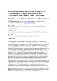
Figure 1: Vertical pr<strong>of</strong>ile computed by the model <strong>of</strong> the ratio between the local ustar <strong>and</strong> the mean w<strong>in</strong>d at<br />
different hours <strong>of</strong> the day <strong>in</strong> the centre <strong>of</strong> the urban area (h is the build<strong>in</strong>g height, 25m).
In Fig. 1 a vertical pr<strong>of</strong>ile <strong>of</strong> the ratio between the local u *<br />
(def<strong>in</strong>ed as<br />
u*( z) = uw() z + vw()<br />
z<br />
2 2 ) <strong>and</strong> the mean horizontal w<strong>in</strong>d computed by the model at<br />
different hours <strong>in</strong> the centre <strong>of</strong> the urban area is presented<br />
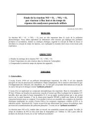
A plot <strong>of</strong> the same variable measured for a series <strong>of</strong> field studies (from Roth, 2000) is <strong>in</strong> Fig.<br />
2. The magnitude <strong>of</strong> the calculated values is comparable with the measurements <strong>and</strong> also the<br />
pr<strong>of</strong>iles have the same behaviour above the ro<strong>of</strong> level. It is <strong>in</strong>terest<strong>in</strong>g to note, also, that below<br />
ro<strong>of</strong> level, there is a decrease <strong>of</strong> this ratio <strong>in</strong> connection with the decrease <strong>of</strong> the Reynolds<br />
Stress as it was measured, for example, by Rotach 1993 <strong>in</strong> Zurich (not shown).<br />
Figure 2: Vertical pr<strong>of</strong>iles <strong>of</strong> the ratio between local ustar <strong>and</strong> horizontal mean w<strong>in</strong>d for different ‘urban’<br />
dataset. From Roth, 2000..<br />
Dur<strong>in</strong>g day <strong>and</strong> night, walls have the biggest impact on the s<strong>in</strong>k <strong>of</strong> <strong>momentum</strong>.<br />
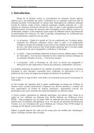
The vertical section <strong>of</strong> the horizontal w<strong>in</strong>d speed (Fig. 3) shows a deceleration <strong>of</strong> the flow<br />
over the urban areas, close to the surface, <strong>and</strong> acceleration above, due to the <strong>heat</strong> isl<strong>and</strong><br />
effects. Dur<strong>in</strong>g night, the effects <strong>of</strong> the town are a reduction <strong>of</strong> the w<strong>in</strong>d speed. Both<br />
phenomena are ‘qualitatively’ <strong>in</strong> agreement with many observations recorded <strong>in</strong> urban areas.
Figure 3: Vertical section <strong>of</strong> the east-west component (parallel to the plane) <strong>of</strong> the mean w<strong>in</strong>d at noon (left) <strong>and</strong><br />
midnight (right). The thick l<strong>in</strong>e on the x-axis represent the urban area.<br />
3.2 Energy<br />
The energy equation is modified <strong>in</strong> the follow<strong>in</strong>g way<br />
∂ρθ ∂ρθUi<br />
∂ρϑui<br />
=− − + H + H + H<br />
∂t<br />
∂x<br />
∂x<br />
i<br />
i<br />
W S R<br />
As it is done for <strong>momentum</strong> it is possible to compute a value for ϑ *<br />
for the street.<br />
H<br />
⎡ S ⎤<br />
S<br />
=−ρu<br />
ϑ ⎢<br />
⎣V<br />
−V<br />
⎥<br />
b ⎦<br />
S * S * S<br />
<strong>and</strong> this is applied only at surface level.<br />
From the value <strong>of</strong>ϑ *<br />
computed for the ro<strong>of</strong><br />
H<br />
=−ρu<br />
R * R * R<br />
⎡SR<br />
⎤<br />
ϑ<br />
⎣<br />
⎢ V ⎦<br />
⎥<br />
this modification is applied at ro<strong>of</strong> level.<br />
For the <strong>heat</strong> <strong>fluxes</strong> from the walls the formulation from Clarke, 1985 was used.<br />
H<br />
w<br />
hc⋅( θ<br />
air<br />
−θ<br />
wall<br />
)<br />
=<br />
C<br />
with<br />
⎛ ⎛<br />
hc = 5. 678⋅ ⎜109 . + 0.<br />
23⋅⎜<br />
⎜ ⎜<br />
⎝ ⎝<br />
p<br />
U<br />
x<br />
+ U<br />
2 2<br />
0.<br />
3048<br />
<strong>and</strong> C p<br />
is the specific <strong>heat</strong> <strong>of</strong> the air.<br />
y<br />
⎞⎞<br />
⎟⎟<br />
⎟⎟<br />
⎠⎠
To compute the surface temperature <strong>of</strong> ro<strong>of</strong>, walls <strong>and</strong> street an energy budget equation is<br />
solved for every surface. The radiation needed for the budget is computed tak<strong>in</strong>g <strong>in</strong>to account<br />
the shadow effects <strong>and</strong> multiple reflections <strong>in</strong> the street canyon.<br />
In Fig. 4 a comparison between the total <strong>heat</strong> storage term computed by the model <strong>and</strong> the<br />
values estimated with the Objective Hysteresis Model <strong>of</strong> Grimmond <strong>and</strong> Oke (which is a<br />
simple parameterisation based on measurements <strong>of</strong> the storage term <strong>in</strong> urban areas as a<br />
function <strong>of</strong> the total radiation) is presented. As it is possible to see the agreement is<br />
particularly good.<br />
Figure 4: Comparison between the total <strong>heat</strong> storage computed by the model <strong>in</strong> the urban area (solid l<strong>in</strong>e) <strong>and</strong><br />
that deduced from the parameterisation <strong>of</strong> Grimmond <strong>and</strong> Oke (crosses) for a three-day simulation.<br />
The analysis <strong>of</strong> the relative importance <strong>of</strong> the different contributions shows that dur<strong>in</strong>g day the<br />
<strong>fluxes</strong> from horizontal surfaces, receiv<strong>in</strong>g more solar energy, are bigger than wall’s <strong>fluxes</strong>.<br />
Dur<strong>in</strong>g night, on the other h<strong>and</strong>, walls are more active than street <strong>and</strong> ro<strong>of</strong>s. This means that<br />
the radiative trapp<strong>in</strong>g plays an important role <strong>in</strong> the <strong>heat</strong> isl<strong>and</strong> phenomena.<br />
The vertical section <strong>of</strong> the potential temperature (Fig. 5) shows a typical <strong>heat</strong> isl<strong>and</strong> effects;<br />
dur<strong>in</strong>g day (the air above the city is hotter <strong>and</strong> the Boundary Layer is higher than <strong>in</strong> the rural<br />
area) <strong>and</strong> dur<strong>in</strong>g night the atmosphere over the city is nearly neutral <strong>and</strong> not very stable as <strong>in</strong><br />
the surround<strong>in</strong>gs.
Figure 5: Vertical section <strong>of</strong> the potential temperature field computed by the model at noon (left) <strong>and</strong> midnight<br />
(right).<br />
3.3 Turbulent K<strong>in</strong>etic Energy<br />
In the prognostic turbulent k<strong>in</strong>etic energy (TKE) equation (formulation <strong>of</strong> Bougeault <strong>and</strong><br />
Lacarrere, 1989) three new terms EW, ES, ERare added<br />
∂ρe<br />
∂ρUe<br />
i<br />
∂ρue<br />
i<br />
=− − + ρK<br />
∂t<br />
∂x<br />
∂x<br />
32 /<br />
i<br />
i<br />
m<br />
⎡⎛<br />
∂U<br />
⎢⎜<br />
⎝<br />
⎣⎢<br />
∂z<br />
x<br />
2<br />
⎞ U<br />
y g ∂∂ ϑ ρ ∂ϑ<br />
⎟ + ⎛ 2<br />
Kh<br />
⎠ ⎝ ⎜ ⎞ ⎤<br />
⎟ ⎥ −<br />
z ⎠<br />
⎦⎥<br />
o<br />
∂ z<br />
− ρC e ε<br />
+ E + E + E<br />
W S R<br />
lε<br />
At the first level the entire equation is solved with a surface flux equal to zero at ground.<br />
The impact <strong>of</strong> the street on the TKE is modelled <strong>in</strong> this way<br />
E<br />
S<br />
3<br />
⎛ u g ⎞<br />
* S<br />
⎡V −V<br />
u<br />
b<br />
⎤<br />
= ρ⎜<br />
− * Sϑ<br />
* S⎟<br />
⎝ vk ⋅ dz / 2 ϑ<br />
⎢<br />
o ⎠ ⎣V<br />
−V<br />
⎥<br />
b ⎦<br />
The first term represents the shear term deduced from surface layer theory us<strong>in</strong>g the value <strong>of</strong><br />
the street friction velocity. The second term is the buoyancy term based on the street surface<br />
<strong>heat</strong> <strong>fluxes</strong>. Both terms are volumetric. Aga<strong>in</strong>, this term is different than zero only at the first<br />
level. dz is the height <strong>of</strong> the grid cell.<br />
Similarly for the ro<strong>of</strong>:<br />
E<br />
R<br />
3<br />
⎛ u*<br />
R<br />
g<br />
= ρ⎜<br />
− u<br />
⎝ vk ⋅ dz / 2 ϑ<br />
o<br />
ϑ<br />
* R * R<br />
⎞ ⎡ Vb<br />
⎟ ⎢<br />
⎠ ⎣V<br />
−V<br />
this term is different than zero only at ro<strong>of</strong> height.<br />
b<br />
⎤<br />
⎥<br />
⎦
The impact <strong>of</strong> the walls is modelled <strong>in</strong> a way similar to what it is done <strong>in</strong> vegetation canopy<br />
models:<br />
3<br />
w drag ort<br />
E = ρC U<br />
⎡ SW<br />
⎢<br />
⎣V<br />
−V<br />
b<br />
⎤<br />
⎥<br />
⎦<br />
In the formulation by Bougeault <strong>and</strong> Lacarrere, the length scales used for the computation <strong>of</strong><br />
the dissipation <strong>and</strong> that for the turbulent diffusion coefficients, are function <strong>of</strong> the TKE value<br />
<strong>in</strong> the po<strong>in</strong>t <strong>and</strong> the pr<strong>of</strong>ile <strong>of</strong> potential temperature.<br />
In the case <strong>of</strong> an urban surface, the presence <strong>of</strong> build<strong>in</strong>gs can <strong>in</strong>duce some circulation <strong>of</strong> a size<br />
comparable with that <strong>of</strong> the roughness element. For this reason, below ro<strong>of</strong> level we added a<br />
second length scale (the roughness element size):<br />
1 1 1<br />
= +<br />
l l hu<br />
B<br />
where hu is the build<strong>in</strong>g’s height <strong>and</strong> l B<br />
is the length scale computed with the orig<strong>in</strong>al<br />
formulation.<br />
Vertical pr<strong>of</strong>iles <strong>of</strong> TKE normalised by the square root <strong>of</strong> the Reynolds Stress at the ro<strong>of</strong><br />
height are shown <strong>in</strong> Fig. 6.<br />
Figure 6: Vertical pr<strong>of</strong>ile <strong>of</strong> the ratio between the turbulent k<strong>in</strong>etic energy <strong>and</strong> the square root <strong>of</strong> the Reynolds<br />
Stress computed by the model <strong>in</strong> the centre <strong>of</strong> the urban area at different time <strong>of</strong> the day.<br />
Those values are consistent with the measurements <strong>of</strong> Rotach (1993) around ro<strong>of</strong> height <strong>and</strong><br />
with that <strong>of</strong> Feigenw<strong>in</strong>ter et al. at 2-3 times the build<strong>in</strong>g height.<br />
As for <strong>momentum</strong>, also for TKE the most active surface is the walls.<br />
4. Conclusions<br />
A parameterisation for <strong>heat</strong> <strong>and</strong> <strong>momentum</strong> <strong>fluxes</strong> for mesoscale models <strong>in</strong> urban areas is<br />
presented. The formulation takes <strong>in</strong>to account separately the impact <strong>of</strong> the three active<br />
surfaces <strong>of</strong> the roughness element: wall, street <strong>and</strong> ro<strong>of</strong>. The modifications were <strong>in</strong>troduced <strong>in</strong><br />
a mesoscale model <strong>and</strong> tested <strong>in</strong> a simple 2D case. A comparison with series <strong>of</strong> field
measurements shows that the new formulation is able to reproduce the ma<strong>in</strong> features <strong>of</strong><br />
<strong>momentum</strong>, <strong>heat</strong> <strong>and</strong> turbulent <strong>fluxes</strong> <strong>in</strong> urban areas.<br />
From the analysis <strong>of</strong> the impact <strong>of</strong> the different terms it is possible to see that the walls are the<br />
most active surfaces for <strong>momentum</strong> <strong>and</strong> TKE dur<strong>in</strong>g the day <strong>and</strong> dur<strong>in</strong>g the night. For <strong>heat</strong>, on<br />
the other h<strong>and</strong>, street <strong>and</strong> ro<strong>of</strong>s are more active dur<strong>in</strong>g daytime <strong>and</strong> walls dur<strong>in</strong>g night-time.<br />
Acknowledgements<br />
The authors would like to thank M. Roth for provides Fig. 2.<br />
References<br />
Bougeault, P. & T. Lacarrere (1989) Parameterization <strong>of</strong> Orography-Induced Turbulence <strong>in</strong> a Mesobeta-Scale<br />
Model, Monthly Weather Review, 117, 1872-1890<br />
Clarke, J. A. (1985) Energy simulation <strong>in</strong> build<strong>in</strong>g design, Adam Hilger, Bristol<br />
Collella, P. & P. Woodward (1984). The piecewise parabolic method (PPM) for gas dynamical simulations. J.<br />
Comp. Phys.., 54, 174-201.<br />
Louis, J. F. (1979) A parametric model <strong>of</strong> vertical eddies <strong>fluxes</strong> <strong>in</strong> the atmosphere, Boundary-Layer<br />
Meteorology,17, 187-202<br />
Raupach, M., R. (1992) Drag <strong>and</strong> drag partition on rough surfaces, Boundary-Layer Meteorology, 60, 375-395<br />
Rotach, M., W. (1993) Turbulence close to a rough urban surface. Part1: Reynolds Stress. Boundary Layer<br />
Meteorology, 65, 1-28<br />
Roth. M. (2000), Review <strong>of</strong> atmospheric turbulence over cities <strong>in</strong> press for Q.J.R.M.S.<br />
Tremback, C., J. <strong>and</strong> R. Kessler, (1985) A surface temperature <strong>and</strong> moisture <strong>parameterization</strong> for use <strong>in</strong><br />
mesoscale numerical models, Proceed<strong>in</strong>gs <strong>of</strong> 7th conference on Numerical Weather Prediction, June 17-20,<br />
Montreal, Quebec, Canada<br />
Uno, I., H. Ueda & S. Wakamatsu (1989) Numerical modell<strong>in</strong>g <strong>of</strong> the nocturnal urban boundary layer,<br />
Boundary-Layer Meteorology, 49, 77-98.<br />
Wilson N. & R. Shaw (1977) A higher order closure model for canopy low, J Appl. Metor., 16, 1197-1205.<br />
Yamada, T. (1982) A numerical study <strong>of</strong> turbulent airflow <strong>in</strong> <strong>and</strong> above a forest canopy, J. Met. Soc. Japan, 60,<br />
439-454