The spatial behavior of residential burglars Manuel J.J. ... - TU Delft

The spatial behavior of residential burglars 

Manuel J.J. López 

RCM-advies, The Netherlands 

m.lopez@RCM-advies.nl 

Abstract 

Criminals live in a built environment and use this environment for their daily activities and 

movement. In many respects they are just like ordinary people. In fact they are ordinary 

people, but with one extraordinary exception. Criminals commit crimes and professional 

criminals commit crimes on a regular basis. This remarkable habit sets them apart from 

the majority. Almost everybody has done something in life that was not quite legitimate. 

We have all stolen a candy bar as a child, thrown a stone through a window when we were 

juveniles, or made up little lies when we had to fill out our tax papers. Testing boundaries 

is human, but knowingly and willingly crossing these borders again and again is what sets 

criminals apart from ‘ordinary’ people. 

If criminals are ordinary people with extraordinary professions, we might wonder what 

consequences this profession has for criminals’ spatial behavior. Do criminal offenders 

use space in exactly the same way as other people or are there notable differences? It 

is reasonable to assume that the special nature of their profession influences the daily 

routines of criminals and that this is reflected in the nature of their spatial behavior? 

To explore these broad questions, the research-and-consultancy firm RCM-advies, the 

Technical University of Delft, and the Dutch police force began a collaborative effort. 

This collaboration is ongoing and will probably lead to putting together more pieces of 

the spatial criminological puzzle in coming years. In 2004 a first step in the study focused 

on the spatial relationship between the places of offender residence and the locations of 

offending. 1 Both sides of the collaboration have a scientific interest in and a preference for 

practical application. Therefore we did not restrict our research to the question: “Is there 

a relationship between the place of offender residence and the locations where he commits 

his criminal offences?” but also asked: “If this is the case, can we use this knowledge to 

make a geographical application that the police can use to improve the efficiency of its 

criminal investigation in catching criminals more rapidly?” 2 

When we take a closer look at the contemporary criminological literature, it seems 

that both questions can be answered positively. There are several criminological theories 

that argue that offenders tend to commit their crimes in spots that are known to them 

from their daily activities and movements. They are especially inclined to commit their 

offenses near their homes and along the routes between their house and the places where 

they regularly work, shop, and enjoy recreation. Empirical data support this view and 

show that the majority of offenders have a strikingly small offending radius. Half of the 

1 This study was conducted in the police region Kennemerland and with financial support of the Police 

and Science Program (PW/OC/2004/08). 

2 In this first presentation, I will address these two questions from a criminological point of view. After 

this, Dr. Akkelies van Nes (TU Delft) will take over to give a similar presentation from a space syntax 

point of view.

424 Manuel J.J. López 

hold-ups in Amsterdam take place within a range of 2.6 kilometers from the home of the 

offender (Van Koppen et al. 2000). The police can exploit these scientific insights and 

use them to catch offenders more rapidly and more efficiently. This form of intelligenceled 

policing is also called geographic profiling. In Canada, the U.S., and Great Britain, 

geographic profiling has been applied successfully by several police forces and has led to 

several profiling techniques and (associated) software. 

1. Criminological theories 

Geographic profiling has its scientific basis in environmental criminology and - more specifically 

- routine activity theory (Felson and Cohen 1998) and crime pattern theory (Brantingham 

and Brantingham 1981; 1993; 1995). These theories argue that criminal offenders 

commit their crimes in spots and places that are familiar to them from daily routine. 

These spots are along the routes between their homes and the places they regularly work, 

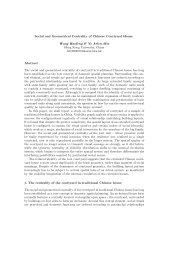
shop, and enjoy recreation. On the way to his local supermarket, a residential burglar 

looks at the houses he passes and gets an idea of available attractive targets. Every time 

he takes this route, he gets to know the area better. He learns, for example, in which 

houses nobody is present during the day, which houses are poorly protected and which 

ones house wealthy residents. “Opportunity spaces” arise on the basis of this knowledge. 

These are spots within the offender’s spatial experience that he assesses as attractive. The 

home of the offender generally forms a central place in his spatial experience (“awareness 

space”). Just like non-delinquents, delinquents spend most of their time in and around 

their homes 3 . The home is, for most of us, both geographically and socially the most central 

spot in our life and forms our geographical operating base. For the offender, the home 

is generally the start and/or end of his criminal journey. This explains why the criminal 

offender commits his crimes in the proximity of his home: in spots that are known to him 

and considered to be attractive. 

The fact that criminals generally commit their offences in the proximity of their homes 

is also well supported by empirical data. Empirical studies do, however, call our attention 

to some important points. Some offenders do not have a steady home address. Moreover, 

there is a category of offenders who are extremely mobile and commit their offences everywhere 

but in the proximity of their homes (Canter and Larkin 1993; Wiles and Costello 

2000). They do not commit their offences near their homes, but in the proximity of other 

geographical anchor points such as their workplace, café, the house of a relative or friend 

(Rengert and Wasilchick 2000), or somewhere in the inner city (Shaw and McKay 1942). 

With regard to numbers, these specific categories of offenders are significant, but nevertheless, 

a minority. Finally, empirical studies show that the distance of travel (the so-called 

“range of operation”) of an offender is everything but constant. The size of this range of 

operation depends on the characteristics of the offender, the offense type, the characteristics 

of the spatial environment, and the prevalent modes of personal transportation. 

Criminological theories not only suggest a range of operation, but also some other 

aspects that influence the relationship between the place of residence and places of offending. 

The first of these aspects is known as the principle of “distance decay.” This principle 

suggests that within a radius, the number of offences will decrease exponentially with 

the increase of travel distance. At the centre of the radius, directly around the offender’s 

3 On average, we spend three quarters of our time in and around our home (Ministry of VROM 2000, 

pg. 15).

The spatial behavior of residential burglars 425 

Figure 199: “Awareness space” and “opportunity space” 

home, there is a reduced likelihood off offending (Turner 1969). The people who live in this 

area (also called the “buffer zone”) are more likely to know the offender than people who 

live a little farther away so there is a higher risk of recognition. Several studies mention 

the importance of travel direction (e.g. Godwin 2000; Lundrigan and Canter 2001) and 

all environmental criminological theories also point to spatial and physical characteristics 

if the built environment is to be taken into account. In sum, criminological theory recognizes 

five parameters that explain the spatial relationship between an offender’s home 

and places of offending. Four parameters - range of operation, distance decay, buffer zone 

and travel direction - are related to the awareness space of the offender. One parameter - 

spatial and physical characteristics of the built environment - represents the opportunity 

space of the offender. 

2. The study 

The parameters that give a theoretical explanation for the spatial relationship between 

an offender’s home and places of offending can easily be tested when we have a database 

of known offenders, locations of their home bases, and locations of their crimes. Such a 

database not only allows us to test the validity of the parameters, but also the validity 

of the different profiling techniques that use these parameters to identify the area within 

which we have the largest probability of finding the offender’s home base. Thus, a database 

was constructed with information of all residential burglars who lived in the police region 

of Kennemerland and who were known to have committed at least 5 burglaries in a period 

of six years (1998 - 2004). The database contained information on the offender’s (present 

and previous) home addresses and the addresses of the residential burglaries for which 

they were convicted. 

The study was based on a sample of 20 residential burglars. All of these burglars lived 

in the police region of Kennemerland during the period of offending and were convicted of


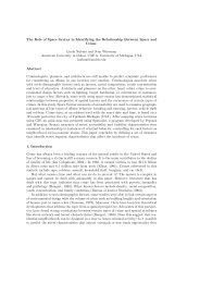
Figure 200: Range of operation and buffer zone 

at least five burglary offences that were committed between 1998 and 2004. When we look 

at the sample, we see that none of the offenders were specialists in the sense that they did 

not limit their criminal acts to residential burglary. They were all male and between the 

ages of 21 and 43. The mean age was 31.8 (S.D. = 0.6). Seven offenders were registered 

by the police as habitual offenders, one was an alcoholic and one was a drug addict. The 

average number of burglary offences by one offender was 11, with a minimum of 5 and a 

maximum of 19 (S.D. = 3.9). Half of the offenders (10) were born in Kennemerland and 

the other half were born elsewhere in The Netherlands (8) or abroad (2). 

A minimum of five maps was made for each offender. The first map showed the different 

home addresses of the offender during his lifetime. A distinction was made between the 

offender’s home address before, during and after the period of offending. The second 

map marked the locations of the burglary offences and the remaining maps gave different 

representations of the relationship between the offender’s home and burglary locations. 

3. Range of operation 

The first step in the study was testing the hypothesis about the range of operation. 

When we know both the location of the offender’s home base and the location of his 

offenses, we can easily determine the range of operation by measuring the longest straightline 

distance between the home location and offence locations. The so-called buffer zone 

can be determined in the same fashion, by measuring the shortest straight-line distance 

between the home location and offence locations. Both the range of operation and the 

buffer zone can be represented on a map, by drawing both distances around the home 

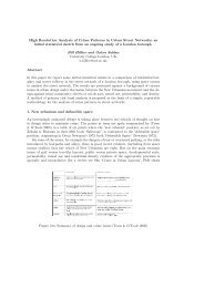
location with a pair of compasses (Figure 200). When we reverse this procedure and draw 

the longest straight-line distance not around the location of the offender’s home but around 

the locations of his offences, we see that the offender’s home base is in the area of the 

biggest overlap (Figure 201). 

If we both know the location of the offences and the distance of the range of operation, 

we can be 100% accurate in defining the area in which we can expect the offender’s


Figure 201: Defining the search area 

home base. However, criminal investigation is not always successful and most crimes are 

not solved. 4 The police may have indications that certain offences are committed by the 

same offender (e.g. through DNA or other clues), but may not know the identity of the 

offender and his range of operation. For such cases we have a couple of techniques that 

can help. Canter and Larkin (1993) measure the maximum distance of offence locations 

within a crime series as the range of operation. This method might seem arbitrary, but it 

is based on the empirical finding that the maximum distance of offence locations usually 

closely matches the longest straight-line distance between the home location and offence 

location (the range of operation). Van Koppen et al. (2000) present another solution. They 

measure all distances between the home and offence locations for every known offender, 

offence type, and geographic area. Then, the median of these distances is calculated. The 

resulting value is the range of operation of all offenders within that geographic area. 

Both methods have their pros and cons. The method of Canter and Larkin is offender 

specific and therefore does justice to the variations of mobility of the different individual 

offenders. This method also often succeeds in identifying the correct search area (the area 

in which the home location of the offender is suspected), but in some cases this area is 

so large that it has no additional value for the criminal investigation. The method of Van 

Koppen et al. is not offender specific as it chooses one range of operation for all offenders 

of a certain offense type in a given geographic area. The advantage of this approach is 

that the range of operation that will be used for criminal investigation is never too big. 

It always produces search areas that are small; thus, they offer additional value for the 

criminal investigation. However, the method also has two major disadvantages. The first 

disadvantage is the fact that it is based on the incorrect assumption that the radius in 

which he commits 50 percent of his offences can identify the offender’s range of operation. 5 

There is also the disadvantage that the method does insufficient justice to the fact that 

different offenders most often have different ranges of operation. Given the disadvantages of 

both methods, this study developed an alternative approach. This third method combines 

the two earlier methods. First, it identifies the median of the ranges of operation of all 

known offenders of a certain offence type in a given geographic area. Secondly, the method 

4 In 2000 the national clearance rate for residential burglary was 7.2% (López and Reijenga 2001). The 

clearance rate in Kennemerland was a little higher as 9.8% of residential burglaries had resulted in 

the conviction of one or more suspects. 

5 The idea to take the median rather than the average is a good one, but should actually be applied on 

the longest distance between the offender’s home and offence locations (the real range of operation).


specifies this for every offence series and thereby for every offender and offense type. This 

is done in two successive steps: 

• The range of operation - for a given offense type and geographic area - is given 

the same value as the median of the maximum distances of offence locations within 

all crime series. In the case of residential burglary in Kennemerland, this is 2.1 

kilometers. 

• If the longest straight-line distance between offense locations within a certain crime 

series has a shorter distance than the median, then the range of operation will be 

given the value of this shorter distance. 

By operating in this manner, we do justice both to the differences in geographic mobility 

of the individual offenders and the wish of criminal investigators to produce a search 

area of a limited size. 

4. Results 

When we take a look at the distances between the offender’s home address and the locations 

of his burglaries, we see that most offenders stay close to home. The average distance 

between the home address and offence location in our sample was 1.72 kilometers. 6 Both 

the median (M.D. = 1.10) and the standard deviation (S.D. = 2.44) show that there are 

considerable differences in the travel distances of the individual offenders. The longest 

travel distances of all crime series varied between 650 meters and 7.8 kilometers, with an 

average of 3.0 kilometers (M.D.= 2.3 and S.D.= 1.9). The longest straight-line distance 

between offence-locations within a crime series closely matched the different ranges of operation 

and varied between 800 meters and 8.7 kilometers. The average of these distances 

was 3.2 kilometers (M.D.= 2.1 and S.D.= 2.2). 

The table in fig 202 shows the results of implementing the three methods. The first 

column shows the identification number of the different offenders. The next column shows 

how many residential burglaries this offender committed in the last six years that were 

solved by the police. The third, fourth and fifth columns show the range of operation and 

the size of the search area that are calculated when we use Canter and Larkin’s method 

and the observation of whether or not the home address can actually be found within the 

identified search area. The sixth to eighth columns give an overview of the same output 

variables when we apply the Van Koppen et al. method. The last three columns show the 

results of the alternative approach. 

If we apply Canter and Larkin’s (1993) method to our 20 burglary series and determine 

the range of operation by measuring the maximum straight-line distance of offence 

locations within a crime series, we see that this results in a correct search area in 16 

out of the 20 cases (80%). At the same time, we see that in five cases the search area 

indeed includes the offender’s home address, but is so large that it is of no practical use 

for criminal investigation. These five cases are marked with exclamation marks in the fifth 

column. Taking these cases into account, we can conclude that the Canter and Larkin 

method leads to a correct and useful search area in 11 of the 20 cases (55%). 

6 This short travel distance is not very surprising when we realize that the sample was based on local 

offenders.


Figure 202: table 

The Van Koppen et al. (2000) method results in much shorter ranges of operation. In all 

cases the radius was 1.10 kilometers. This also results in search area that are much smaller 

than the Canter and Larkin method. In 9 out of 20 cases, we indeed find the offender’s 

home address in the identified search area (45%). All these area are small enough to be 

useful for criminal investigations. 

The alternative method formulated in this study result in 16 of the 20 cases (80%) 

in search area that include the offender’s home address. In two cases, the search area is 

correct but larger than 2.0 x 2.0 km. When we also take these cases into account, we can 

say that the alternative method leads to a correct and useful search area in 14 of the 20 

cases (70%). These area both contain the offender’s home address and are small enough 

to be useful to criminal investigations. In 10 out of the 14 cases the search area identify 

the address where the offender was living at the time of the burglaries. In two cases the 

search area is found around a past home address. In 3 cases (19%) the search area includes 

an address where the offender would be registered shortly after the burglaries. 7 

5. Distance decay 

Now that we know that 80% of the residential burglars of Kennemerland commit their 

offences within a range of 2.1 km, we may ask ourselves whether they do so at random 

distances or whether there is also a correlation between travel distance and offending 

within the range of operation. Criminological literature most consistently points out the 

7 The data on the offender’s home addresses are derived from municipal population registrations. It 

is mandatory for Dutch citizens to report any changes to a home address in a timely manner. It 

is, however, not uncommon for citizens to make such reports after (sometimes long after) they have 

actually moved.


Figure 203: Distance decay. The relation between the number of offences and normalized 

travel distances 

existence of the so-called distance decay function. This function tells us that most offenders 

commit their offences close to their home and that the longer the travel distance the less 

offences are committed (Phillips 1980). There is, however, one important exception to 

this rule. Offenders do not commit their crimes on their doorstep (Turner 1969). At the 

centre of the radius directly around the offender’s home, is a “buffer zone” with a reduced 

likelihood of offending because the offender is at a higher risk of recognition. Both the 

distance decay function and the buffer zone are thought to be the result of rational choice 

behavior of the offender in which the offender tries to find a safe way to maximize his 

profit by means of the smallest possible effort (Cornish and Clarke 1986). 

But how real is distance decay and do offenders really have a buffer zone? Van Koppen 

and De Keijser (1996) are skeptical about both concepts and consider them the results 

of an aggregation-fallacy. “The aggregated distance-decay function is an inevitable effect, 

as we will show, of including in the analyses offenders with varying ranges of operation. 

Irrespective of differences in offense-density (the range divided by the number of offenses), 

the relatively smaller ranges included in the data will aggregate to form a peak at the 

lower side of the distance scale although none of the individual offenders’ behaviors might 

be characterised by distance-decay properties. The transition from individual no-decay 

functions to an aggregated distance-decay function is thus an aggregation-fallacy.” (Van 

Koppen and De Keijser 1996, pg. 6). 

The idea of distance decay is not one without controversy. If we want to test the 

distance decay hypothesis we must avoid the aggregation-trap. Therefore it is better to 

use normalized distances in place of metric distances. These distances can be calculated 

by taking the metric distance between an offender’s home and his place of offending and 

dividing this by the maximum of these personal distances. By doing so we get the relative 

distance between his home and offense location for each offender and each offense type, 

expressed by a number between 0 and 1. When we put all normalized distances of all 

offenders in one graphic representation, we get insight both into the existence and shape 

of the distance decay-function and the possible presence of opportunity spaces. 

If we carry out the described procedure, we get the following figure (Figure 203). 

Figure 203 shows that the presence of a distance decay-function is not supported by 

the available data. At the same time, we also do not see an even distribution of offences. 

There are several spikes in the figure that indicate that certain distances (especially at 

normalized distances .1, .6 and .9) contain more residential burglaries than other distances.


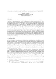
Figure 204: The relationship between farthest offense distance and range of operation 

This is a strong indication for the presence of opportunity spaces (i.e., spaces within the 

range of operation that are considered by the offender to be more attractive than other 

spaces). 

6. Buffer zone 

Canter and Larkin (1993) studied the geographic distribution of crimes committed by 

serial rapists and tested the validity of the different hypotheses on the buffer zone and the 

suspected relationship between the farthest offence distance within a crime series and the 

range of operation that were formulated by Brantingham and Brantingham (1981). This 

was done by transforming the Pareto-function y = k/xb + c into the regression y = ax + c. 

Variable a in this equation, the gradient, has a value between 0 and 1.0. An a < 0.5 tells us 

that the assumption about the range of operation (the so-called ‘circle-hypothesis’) has to 

be rejected. If a=0.5 we know that the offender’s home address is exactly in the middle of 

the radius and an a between 0.5 and 1.0 shows us that this is not the case. In this last case, 

we know that the higher the value of a the longer the distance between the middle of the 

radius and the offender’s home address. Constant c indicates the radius of the buffer zone. 

The buffer zone-hypothesis is accepted when c has a positive value that is smaller than 

the average straight-line distance between the home and nearest offense location. Canter 

and Larkin tested the different hypotheses by scatter plotting the maximum distance of 

offence locations against the longest straight-line distance between the home location and 

offence locations (the range of operation). 

If we follow the same procedure with our crime data and we normalize the distances 

to values between 0 and 10, we get the following scatter plot (Figure 204). 

The correlation between the two variables is both strong (r=0.88) and significant (p < 

0.001). The regression function is y = 0.87x + 0.15. The gradient of 0.87 tells us that the 

circle-hypotheses is accepted, but also that the offender’s home address is not exactly in 

the middle of the radius. The constant has a value of 0.15. This is a lower value than 

the average distance between the offender’s home address and the nearest offence location 

(0.25), so we must conclude that the hypothesis about the buffer zone is accepted but 

also that the buffer zone is extremely small (150 meters). When we take a close look at


our crime series, we see that 4 out of 20 offenders committed residential burglaries on the 

street where they lived. Two offenders even committed burglaries in the homes of their 

former neighbors. These facts are not in line with the theories that assume the existence 

of a buffer zone. 

7. Travel direction 

By only looking into the offender’s range of operation, distance decay, and buffer zone, 

we make the implicit assumptions that offenses are evenly distributed within the range of 

operation and that the home of the offender will be exactly in the middle of the offence 

locations. We have seen however, that these assumptions are not correct. The offender’s 

home address is often not exactly in the middle of the offence locations and some distances 

contain more offences than others. This can be caused by the non-random distribution 

of opportunity spaces, but it can also be caused by the fact that burglars have some 

favorite travel directions, for example, because the locations of their work, recreation 

and/or shopping happen to be in those directions. The presentation of Akkelies van Nes 

will deal with the possible influence of the built environment (and the related distribution 

of opportunity spaces) on the offender’s spatial behavior. First, however, we will take a 

closer look into a possible alternative explanation; namely the offender’s preference for a 

certain travel direction. 

According to Lundrigan and Canter (2001), the hypothesis about the offender’s directional 

preference can best be tested by analyzing the angles created by the offender’s 

home and his offence locations. The hypothesis is confirmed when the angle is smaller 

than 90o (a sharp angle). If the angle is bigger than 90o, we must reject the hypothesis. In 

that case, we have found proof that the offender does not have any directional preference. 

Godwin (2000) follows a comparable approach and calculates the directional angle on the 

basis of the geographical degrees of longitude and latitude. Both studies show that serial 

killers and (in the case of Godwin’s study) serial rapists have a clear directional preference 

when committing offences. This is important information for geographic profiling, since it 

aids in restricting the size of the search area. 

However, residential burglars are (in most cases) not serial killers. And we have seen 

that some aspects of the spatial behavior of offenders (e.g., travel distance) are influenced 

by factors that are related to the offence type. For this reason, we should not automatically 

assume that conclusions about the directional preference of serial killers and serial rapists 

also apply to serial residential burglars. At present, there is no empirical evidence that 

proves that residential burglars do or do not have a directional preference. The study from 

Barker (2000) seems to suggest such a preference, but provides insufficient evidence. 

When we apply the method of Lundrigan and Canter (2001) and calculate the directional 

angle of the crime series, we see that the residential burglars in our sample do not 

have a preference for a certain travel direction. There is only one crime series in our sample 

with a directional angle smaller than 90 o . This relatively small angle (35 o ), however, 

seems to be the result of the small number of offences in the crime series rather than the 

personal preference of the offender for a certain direction. Nine of the 17 crime series even 

show angles of 180 o or bigger.


Table 21: Directional angle by offender 

Offender Radius Number of offences Directional angle 

5 1.4 11 110 o 

6 0.8 6 95 o 

11 1.5 17 200 o 

12 1.4 11 220 o 

13 1.8 15 125 o 

14 1.9 11 250 o 

16 2.0 5 180 o 

17 2.0 11 120 o 

19 0.8/2.1 19 245 o 

20 1.8/2.2 12 265 o 

23 1.4 7 245 o 

25 1.4 11 110 o 

30 1.0/3.3 16 210 o 

33 2.1 8 170 o 

35 2.0 9 120 o 

36 0.8 13 260 o 

37 2.0 5 35 o 

8. Conclusions 

In this presentation, we formulated some basic questions about the spatial relationship 

between the criminal offender’s home address and the location of his offences, and tried to 

find the answers from a criminological perspective. In the next paper, Dr. Akkelies van Nes 

presents a similar contribution, but from a space syntax point of view. The purpose of this 

co-presentation is to bring environmental criminology and space syntax closer together, 

about which we feel strongly. When I read about the subject of space and crime, I am 

always struck by the lack of criminological theory in the work of space syntax researchers. 

If they mention theories, they always refer to Jane Jacobs (1961) and the early work of 

Oscar Newman (1972). By doing so, not only do they do an injustice to Oscar Newman 

(who radically revised his theories in 1980), but also to criminology in general, which has 

evolved dramatically since the 1980’s. However, ignorance also works both ways. When I 

read studies on environmental criminology, I hardly ever see any reference to space syntax 

research. Both disciplines have many common interests, but the connecting link is rarely 

made. van Nes and I hope to make a small contribution in bridging the gap between our 

two disciplines. 

What have we learned so far? First of all, I think we can all agree that the two questions 

formulated at the beginning of my presentation have been answered affirmatively. 

• 1. Is there a relationship between the place of offender residence and the locations 

where he commits his criminal offences? Yes, there most certainly is. There is a 

category of offenders who are extremely mobile and there is a category that doesn’t 

have a steady home address. But when we look to residential burglars in Kennemerland 

we must conclude that the majority commit offences in close proximity of their 

homes (within a range of 2.1 kilometers). Some theories and studies suggest the existence 

of a buffer zone, a distance-decay function and a directional preference, but


these suggestions are not supported by our data. 

• 2. Can we use the findings of this study and make a geographical application that 

the police can use to improve the efficiency of criminal investigations and catch 

criminals more rapidly? Yes we can. There are several techniques to establish the 

geographic profile of an offender. Some techniques are extremely simple while others 

are so complex that they require the utilization of specialized computer software. 

However, more complex is not always better. The current research shows that the 

simplest technique that establishes the geographic profile of an offender (the circle 

technique) is preferable to more complex ones. Presently, there are several commercial 

computer systems that produce maps that indicate the most probable area 

of offender residence. These systems require considerable financial investment and 

police officers must receive specialized training before they are able and allowed to 

use the computer software. It is doubtful whether the commercial computer systems 

offer any added value. Models that try to improve the results of the circle technique 

(e.g., by taking into account one or more distance decay functions, a buffer zone 

and/or a specific travel direction) are not likely to improve the result of geographic 

profiling. 8 

This presentation was limited to the parameters that are related to the awareness 

space of the criminal offender. The influence of the opportunity space was left out of the 

equation and spared for the presentation of Akkelies van Nes. We did so because the 

presentation of van Nes will show that the spatial and physical characteristics of the built 

environment (opportunity space) have an important influence on the criminal behavior of 

offenders. Offenders, like residential burglars, know their territory well and can indeed be 

defined as “space explorers” (Hillier 1996). Can this help us and aid us in our quest for 

better and more powerful techniques of geographic profiling? I am convinced that it can. 

However, let us first listen to van Nes to gain an understanding of the precise relationship 

between criminal opportunity and the spatial characteristics of the built environment. 

Literature 

Barker M., (2000) The criminal range of small-town burglars, in: D. Canter en L. 

Alison, Profiling property crimes, Liverpool: Ashgate Dartmouth, p. 57-73 

Brantingham, P. and Brantingham, P. (1981) Environmental Criminology, Sage 

Publications, Bevery Hills, Sage. 

Brantingham, P. and Brantingham, P. (1984) Patterns in Crime, Macmillan Publishing 

Company, New York. 

Brantingham, P.L. en P.J. Brantingham, (1993) Nodes, paths and edges: considerations 

on the complexity of crime and the physical environment, in: Journal of 

Environmental Psychology, nr. 13, p. 3-28 

Brantingham, P.L. en P.J. Brantingham, (1995) Criminality of place: crime generators 

and crime attractors, European Journal on Criminal Policy and Research, 

Vol. 3, nr. 3, p. 5-26. 

8 See also the study of Snook (2000) in which students were informed about the principles of distance 

decay and the range of operation. Students were able to define search areas on a map that were as 

accurate as the computer program Dragnet.


Canter, D. en P. Larkin, (1993) The environmental range of serial rapists, Journal 

of Environmental Psychology, nr. 13, p. 66-69. 

Cornish, D.B. en R.V. Clarke, (1986) The Reasoning Criminal Rational Choice 

Perspective on Offending, New York: Springler-Verlag. 

Felson, M. and L.E. Cohen, (1998) Human ecology and crime: a routine activity approach, 

Human Ecology, Vol. 8, nr. 4, p. 389-405. 

Hillier, B., (1996) Space is the Machine, Cambridge: Cambridge University Press. 

Jacobs, J. (2000) The Death and Life of Great American Cities, London: Pimlico. 

Koppen, P.J. van en J.W. de Keijser, (1996) Desisting distance-decay, Leiden: 

NSCR/NISCALE. 

Koppen, P.J. van, J.J. van der Kemp en C.J. de Poot, (2002) Geografische 

daderprofilering, in: P.J. van Koppen, D.J. Hessing, H. Merckelbach en H.F.M. 

Crombag (red.), Het recht van binnen: Psychologie van het recht, Deventer: Kluwer, 

p. 237-254. 

López, M.J.J. en P.T. Reijenga, (2001) Doorbraakmeter. Tussentijdse evaluatie van 

de uitvoering van het Kwaliteitsprogramma Veilig Wonen 1997-2001, Den Haag: 

Expertisecentrum Woningcriminaliteit. 

Lundrigan, S. and D. Canter, (2001) Spatial patterns of serial murder: an analysis 

of disposal site location choice, Behavioral Sciences & the Law, Vol. 19, nr. 4, p. 595 

- 610. 

Newman, O. (1972) Defensible Space. Crime prevention through urban design, Macmillan 

Company, New York. 

Newman, O. (1980) Community of interest, Anchor Press, Doubleday, New York. 

Ministerie van Volkshuisvesting, (2000) Ruimtelijke Ordening en Milieubeleid 

(VROM), Mensen wensen wonen: Wonen in de 21e eeuw, Den Haag: VROM 

Phillips, P.D. (1980) Characteristics and typologie of the journey to crime, in: D.E. 

Georges-Abeyie and K.D. Harries (eds.), Crime. A spatial perspective, New York: 

Colombia University Press, pg. 167-180. 

Rengert, G.F. and J. Wasilchick, (2000) Suburban burglary: a tale of two suburbs, 

Springfield, IL: Charles C. Thomas. 

Shaw, C.R., and H.D. McKay, (1942) Juvenile Delinquency in Urban Areas, 

Chicago: University of Chicago Press. 

Snook, B. (2000) Utility or futility? A provisional examination of the utility of a geographical 

decision support system, paper for Wheredunit?: Investigating the role 

of place in crime and criminality, San Diego California, Liverpool: University of 

Liverpool. 

Turner, S., (1969) Delinquency and distance, in: M.E. Wolfgang and T. Sellin (eds.), 

Delinquency: Selected studies, New York: John C. Wiley, p. 11-26. 

Wiles, P. en A. Costello, (2000) The ‘road to nowhere’: the evidence for travelling 

criminals, London: Home Office Research Studie, nr. 207.

The spatial behavior of residential burglars Manuel J.J. ... - TU Delft

You also want an ePaper? Increase the reach of your titles

Delete template?

Save as template?