High Resolution Analysis of Crime Patterns in Urban Street Networks

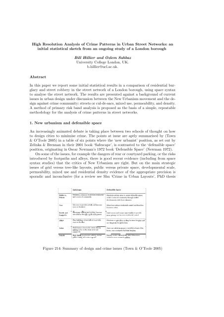
452 B. Hillier and O. SahbazUniversity of London 2000). What is needed is high resolution analysis of crime patternsin urban street networks in which these issues are variables to begin to build the body ofevidence needed to decide these issues. In this paper we propose such a high resolutiontechnique. The unit of analysis is the segment of a street between junctions, and thetechnique combines space syntax analysis with Geographical Information Systems (GIS).In contrast to most available crime analysis packages, which focus on the clusteringof crime in particular locations, space syntax research has pointed to the importance oflooking at non-clustered patterns, that is the kinds of locations in which certain kindsof crime occurred, but which are dispersed throughout the grid and so do not appear asclusters or ‘hot-spots’. By combining space syntax with the data handling capabilities ofGIS, a flexible method of analysis can be developed which works at the high resolutionlevel required, but can also work at higher levels of aggregation such as the Output Areaof the 2001 Census or the administrative divisions into wards.Previous space syntax studies have confirmed some of the principles of the prevailingdefensible space orthodoxy, but has also opened up a positive window on certain newurbanist propositions. For example, syntax studies of residential burglary have confirmedthat when embedded in an urban street network, simple linear cul-de-sacs can often bethe safest places, but that when the cul-de-sac is generalised into a design principle sothat whole areas take the form of a hierarchy of cul-de-sacs, the effects can be quite theopposite (Hillier and Shu 2000, Hillier 2004). It has also shown that in residential areas,the streets that are most integrated - and therefore with more natural movement- areoften safer than the more broken up spaces, but that where integrated streets have ‘localvulnerability’; for example through ‘secondary exposure’ through alleys or adjacent openareas, or basement access, then integrated streets can become singularly vulnerable. Wecall these switches ‘flip over effects’ to express the idea that design variables do not actindependently, but interact, so that all must be got right together if there is to be agenuine reduction in vulnerability. Equally complex results have come from looking atcrimes against the person in urban areas, with patterns of crime shifting with time of dayand thus with the presence of greater or lesser degrees of movement (Alford 1996).But space syntax has not so far studied patterns of crime either at the much largerscales of the city and its multiplicity of socially and spatially differentiated areas, or with afull analysis at the high resolution level of the street segment. In this paper we seek remedythis deficiency by reporting the first results of a space syntax study of crime in the streetnetwork of an entire London borough, with 99,991 households and 263,464 people withinits boundaries (according to Census 2001). We have been given access to a 5 year crimedata base in which every crime has been located and by linking this to a space syntaxanalysis of the whole borough (in the context of its urban surroundings), and linking bothto social and demographics data available from the 2001 census, as well as the Borough’sown property database, we have perhaps the largest and best body of spatial, sociodemographicsand crime data yet brought together in a single study. As an extra bonus,the fact that the London borough in question is largely made up of traditional housingon a street network, makes this data base ideal for posing the key current questions as tohow street networks and their functioning shape the pattern of crime. But we should alsoissue a ‘health warning’. The London borough in question is socially and ethnically highlyvaried, and differentiated physically between its inner, more ‘inner city’, and outer, moresuburban, areas. Some of its centres are already known as high crime areas. We should becareful not to generalise its results prematurely, before a range of such studies have beenmade in different cities.

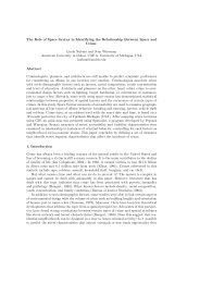
High Resolution Analysis of Crime Patterns in Urban Street Networks: an initialstatistical sketch from an ongoing study of a London borough 453Figure 215: Newman’s Hierarchy image.2. Theoretical background: the other side of NewmanThe key issue in the debate between new urbanism and defensible space is the relationbetween the dwelling and the public realm. Throughout the history of urbanism, thisrelation has been more or less direct, and it would not be an exaggeration to say that thevery basis of urban form historically is dwellings opening on to linear spaces linked intonetwork: the street network. In modern times, this relation has been broken twice: firstby architectural modernism, especially in its social housing programmes (for a review seeHillier 1988); and then by Oscar Newman’s hugely influential ‘defensible space’ concept,as summarised in figure 215, redrawn from page 9 of his book:But in spite of the fact that his concept radically disrupts the dwelling-street relation,throughout his book, when talking about real cities, Newman again and again acknowledgesthe security benefits of well-designed streets with dwellings opening on to them:‘...streets provide security in the form of prominent paths for concentrated pedestrianand vehicular movement’ (op. cit p. 25)....‘the street pattern , with its constant flow ofvehicular and pedestrian traffic, does provide an element of safety for every dwelling unit’(p. 103). He criticises the modernist practice of closing off streets the make larger urbanblocks, noting that ‘An inhabitant returning home must leave the public street and windhis way through the undefined and anonymous grounds of the project to reach the frontdoor of the building. He would have been much safer had he been able to go directly fromstreet to front door, and safer still if the front door and lobby of his building faced directlyonto the street’(p. 25). Later he adds: ‘The interior of project buildings and grounds sufferthe unique distinction of being public in nature and yet hidden from public view’ (p.32) and later still: ‘Large super-blocks, at various densities, have been found to exhibitsystematically higher crime rates than projects of comparable size and density that havecity streets continuing through them’. There is also the reverse effect, that Newman acknowledges:that dwelling entrances on the street benefits the street and makes it moresecure: ‘The street comes under surveillance from the building, the building entries andlobbies under the surveillance of the street’ (p. 15) ‘The positioning of front entrancesalong the street provides them with continuous natural supervision by passers by; the residentswithin their houses, in turn, provide these passer-by with protective surveillance’.There is also a policing benefit: ‘Well lit front door paths, with individual lights over the

454 B. Hillier and O. Sahbazentrances, allow cruising police to spot at a glance any peculiar activity taking place on arow-street house’. And more generally: ‘The street, without the continued presence of thecitizen, will never be made to function safely for him’ (p. 15).One might then ask why Newman to universalise his defensible space concept. Severalfactors seem to have been involved. First, Newman’s object of concern was not the city asa whole but the socially disastrous social housing estates that had been inserted in decadesfollowing the two post-second world war. Second, the idea of hierarchically ordered spacewas at the time the prevailing architectural orthodox, taught in architecture schools underthe rubric of the need for a ‘hierarchy of space from public to private’, which seemed tobe confirmed by the then fashionable, though now largely discarded, ‘theory of humanterritoriality’ (Hillier & Hanson 1984). Newman also thought we might need to movetowards a city of hierarchically ordered enclaves as a kind of spatial counterweight towhat he saw as the increasing openness, liberality and moral heterogeneity of modernsocieties, which he thought had diminished our powers to act as communities and inhibitcrime.Whatever the reasons, the problem situation has now changed. We are no longer preoccupiedwith the need to fix past architectural errors, but to learn to design cities again.The ‘other side of Newman’, and how we link residential areas together to form a wellworkingand secure system, is a key part of this agenda. The aim of this paper is to openup research on this ‘other side of Newman’ from the point of view of urban security, and tobegin to ask how far his many observations on the security benefits of well-working streetnetworks can be supported by evidence. We also have the methodological aim of settingup simple and repeatable space syntax based methods of analysis for crime patterns instreet networks, so that evidence can be accumulated on a consistent basis.3. Redefining the urban crime problemUnderstanding the relation between the urban street network and crime is not simply amatter of measuring properties of the street network and correlating them with levels ofcrime. Cities are highly differentiated spatial systems, with huge variations in movementand activity levels, built form densities and mixes of land use, from one part to another.These variations will inevitably influence crime rates, if for no other reason than that thereare far more opportunities for crime in some areas than others.But there is a more fundamental relation between the differentiation of urban areas andthe street network. In their very nature, cities are dynamic, movement based systems, andmovement is shaped in the first instance by the configuration of its street network (Hillieret al. 1993, Penn et al. 1998a 1998b, Hillier and Iida 2005). Through its configuration,the street network creates a basic pattern of movement flows, and these then shape landuse choices, according to the need for different land uses to be close to or remote frommovement. This sets in train a process that eventually gives rise to a city as a network ofbusy and quiet zones, focused on centres at different scales set against a background ofthe residential space which makes up the bulk of the city. The functional differentiationof the system has its origins in the configuration of the street network itself.Evidence of this ‘city-creating’ process is easy to find in the Borough. If we comparesegments with 1-5 non residential units with those without any, we find on average theylie on longer and more globally, but not locally, integrated lines. If we raise the thresholdwe find that on average segments with 5-20 non-residential units lie on much longer,

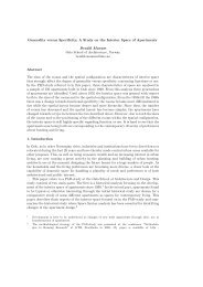
High Resolution Analysis of Crime Patterns in Urban Street Networks: an initialstatistical sketch from an ongoing study of a London borough 455Figure 216:much more connected, and on much longer and more globally integrated lines than thosewithout, but also much more locally integrated and on much more connected lines. Thisis in accordance with the theory which expects that although small numbers of nonresidentialunits such as shops may initially cluster at more globally integrated locationssuch as road intersections, more substantial development of non-residential ‘live’ uses suchas retail requires local integration conditions also to be satisfied. (Hillier 1999) It shouldbe noted that this is found even though we are not yet distinguishing between ‘live’,that is, movement dependent non-residential uses, such as retail and catering, and nonmovementdependent uses. We can expect these differences to be even more marked whenthis distinction is made.The implication of this is that the configuration of the street network and its land usepatterns, together with the movement patterns which link one to the other, are all boundtogether in creating the city as a functionally differentiated system, with large fluctuationsin the density of activities, buildings and movement rates from one area to the next, andeven from one street to the next. The fact that all of these factors, each of which have beenseparately canvassed as being related to crime, are thoroughly inter-correlated through theprocess which creates the functionally differentiated city, warns us to take great care inusing multivariate statistics to establish anything like a chain of causality between thesefactors and crime.4. The street segment levelFrom the point of view of analysis in which the unit of analysis is the street segment, theimplications of this process even more marked. Before we consider the syntactic propertieswhich define how the segment is embedded in the larger scale spatial network, the segmenthas in itself certain basic properties, namely it connectivity, its length, and the number ofbuildings of different kinds and uses that lie on it. Segment connectivity normally has avalue between 1 for the last segment in a cul-de-sac and 6 for a grid like layout, as shownin Figure 216:Segment connectivity thus relates to access and egress (and so to potential escaperoutes), and it the key to the whole issue of grid-like versus tree-like layouts. Other prop-

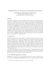
High Resolution Analysis of Crime Patterns in Urban Street Networks: an initialstatistical sketch from an ongoing study of a London borough 461in segments which are less connected, but significantly longer than those without, and alsoon lines which are both significantly longer and more connected hen those without, andsignificantly more integrated locally and globally. Comparing the two crimes, we can saythat robbery is a significantly more integrated crime than burglary, and this is alreadyclear from Figures 219 and 220.7. Disaggregated analysis: the concept of primary risk bandsOur aim here, however, is to relate the pattern of crime to the micro properties of the streetnetwork, and to do this we must establish a unit of analysis and a rate. In previous studiesof burglary (Hillier and Shu 2000) and robbery (Alford 1996), the unit of analysis has beenthe line. This is a rather gross element, which can differ quite considerably in spatial andfunctional properties along its length, so a more micro-scale element would be better. Forburglary, previous syntactic studies have also used the single dwelling as the unit, withspatial differences of the street segment on which it lies assigned to the dwelling. Thispermitted the use of logistic regression to establish the burglary risk associated with eachvariable. However, for our present purposes, there is no robbery equivalent to this becausethe target is an individual rather than a building, and we cannot compare robbed andunrobbed people in the same way that we can compare burgled and unburgled dwellings.The obvious micro unit of analysis is the street segment, which is already the basic unitof the spatial analysis of the street network. But this would only be meaningful if we couldestablish a rate for each crime for a segment, and this is highly problematical. For burglary,for example, however we define a unit of analysis above the level of the individual house- the segment, the street, the block, the administrative area, the geometrically definedquadrant, and so on - then a primary factor influencing the number of burglaries withinthat unit will be the number of residences, or targets, within the unit. This can be shown byconsidering a random pattern. If there is a random pattern of burglary - say by assigningeach house a random number and using a random number selector to select ‘burgled’houses - then as the number of burglaries increases there will be more in units with moreresidences. So in terms of absolute numbers it will appear that there are ‘more’ burglariesin units with more residences. If we then try to correct this by expressing burglary as arate dividing the number of burglaries by the number of residences, then in the early stagesof the process, and perhaps for much of the process, then units with more residences willappear to have lower rates, because the number of residences is now the denominator, andso each randomly assigned ’burglary’ will contribute less to the ‘rate’, and it will appearthat units with more residences have lower rates. We can show this graphically by simplyplotting the count of burglaries per segment against the rate (number of burglaries overnumber of residences) for all street segments in the Borough (Figure 223).We see that all the highest count segments have relatively low rates and all of thehighest rate segments have relatively low counts. We cannot then use either meaningfullyfor statistical analysis. But if we try to standardise the number of residential units, as inthe Output Areas of the 2001 Census for example, then we can only do so by sacrificingconsistency in the spatial descriptors of our unit. Output areas often combine dwellingsfrom main streets, a back street, and maybe also a cul-de-sac, so the spatial coherence ofthe unit is lost.However, we can escape this problem by aggregating all segments with a given numberof residential units, or within a certain band of residential units, and calculating a burglary

462 B. Hillier and O. SahbazFigure 223: Count and rate of burglaries.rate is for the whole group as the total number of burglaries over the total number of targetsfor that group. The number of targets on a segment is now a spatial condition for the unit,and so not involved in the rate calculation at the level of the segment. Because the numberof targets on the segment is the most primitive expression of risk, grouping segments intobands according to the number of targets they represent is the natural way of aggregatingthe data since only in this way can this most fundamental dimension of risk containedwithin the data in a fully transparent way. We can call these aggregates primary riskbands, and note it is rather like taking all the segments that have the condition of having1, 2, 3..... n residential units lying on them and treating them as an imaginary single lineseveral kilometres long. This procedure will of course entail dangers, in that aggregatingdata in this way will also implicate other variables with which they are correlated, whichcould then operate as hidden variables in any subsequent analysis. However, since our aimwill be exactly to investigate the relation between the ‘primary risk’ variable and othervariables, this danger should be minimised.We therefore aggregate the data into sets made up of segments with 1 dwelling (ofwhich there are 328), with 2 (357), and so on up to 30 at which point we take pairs tokeep samples large enough, and increasing the band size to maintain sample size, with afinal band of 90+ (where there are only 34 segments, but with 3708 houses), we end upwith a data table with 47 rows, most of which represent 1000+ houses, and those whichdo not have several hundred. We then for each band take the total number of burglariesand divide by the total number of houses, and so establish a true rate of burglary fordwellings lying on bands with different numbers of target residential units. We show thespatial distribution of the primary risk bands by plotting number of residential units ona segment map of the whole area as in Figure 224.We can see that segments with the lowest number of residential units, tend to be foundfor the most part in high street areas (apart from the business estates), where the lownumber of residential units will be because there are large number of non-residential units,and in parts of the network where space is broken up, including in some social housingestates. In either circumstance, residential units will be relatively isolated, or sharing asegment with very few other residential units. The grey segments are those in which thereare no residential units.8. Primary risk band analysis of burglaryWe then plot two things in the line charts below in which the horizontal axis is always thenumber of dwellings per segment, in each case taking moving averages with a period of 3

464 B. Hillier and O. SahbazFigure 226: segment connectivity and b: Global integration in primary risk bands.There are two possible interpretations of this. The first is natural surveillance: thatmore ‘line neighbours’ in your home segment provide increased surveillance, and that thisdeters burglars. The second is complementary to the finding of Bowers (Bowers, Johnsonand Pease 2004) that the occurrence of a burglary in a location increases the probabilityof further burglaries in the vicinity of the first. If there were an upper limit to this process,then after a certain number of burglaries in a location, the location is seen as saturatedand the risks increased, so the burglar moves on. This would raise interesting psychologicalquestions as to how burglars identify ‘locations’ within which to select a target. The streetsegment is a natural locational unit in the same sense that a street is. Any upper limitto how frequently a burglar saw it as good sense to select targets in the same ‘location’,however defined, would imply greater ‘safety in numbers’ in that location. This findingsuggests that burglars may identify street segments are locations.Whichever interpretation is the case, it means that in an important sense, having moreneighbours helps to keep you safe. The first consequence of adopting the primary risk bandapproach, then, is to bring to light a fundamental regularity in the spatial distribution ofcrime whose existence has been suspected before, but never demonstrated. On this basis,we can then explore the relation of this regularity to other spatial properties. For example,we already know that segment connectivity is found on both short and long segments. Ifwe plot this for the primary risk bands (form left to right on the horizontal axis as before)find that there is high connectivity with few residences per segment, which falls to a low inmid-range, and then rises to high connectivity again for high residence segments. Figure226 shows that the high connectivity segments are to be found both in the high streetareas, where there are few dwellings because most units are non-residential and burglaryrates are among the highest, and in some of the more integrated and grid like housingareas, where burglary rates are among the lowest.We find Figure 226a above an even more striking fall and rise with global integration.This shows that although on average for the whole system segments with burglary are moreglobally integrated than those without, this average conceals a bifurcation in the data.Both high and low burglary rates are associated with integration; high in the integratedhigh street areas where there are few residential neighbours, and low in the integratedresidential areas, where there are many line neighbours. This bifurcation can be showngraphically by a regression plot of integration against the true burglary rate for the primaryrisk bands as in Figure 227 below:If we split the bands more or less evenly between the lower and higher residencebands and plot them separately (Figure 228a and 228b) we find that while for the low

High Resolution Analysis of Crime Patterns in Urban Street Networks: an initialstatistical sketch from an ongoing study of a London borough 465Figure 227: Global integration and rate of Burglary.Figure 228: a and b: Burglary rate of higher and lower residence bands.residence bands more integration means more burglary, for the high residence bands moreintegration - and so more natural movement - means less burglary, though less strongly.This would seem to explain why in previous studies of residential areas integration wasgenerally found, other things being equal, to be associated with lower rates of burglary.We can use the same approach to explore the impact of non-residential land uses onburglary. We find, for example, that although the average number of non-residential landuses increases more or less pro-rata with the increase in the number of residential units,the ratio of non-residence to residence falls consistently throughout the range, as in theleft line chart below (Figure 229).We also find that although segment connectivity and global integration fall then risestrongly with increasing dwellings per segment, the connectivity of the lines on which segmentslie falls consistently, as in the right line chart above, and local integration followsa similar pattern, though in this case with a slight upturn in the high residence ranges.Figure 229:

High Resolution Analysis of Crime Patterns in Urban Street Networks: an initialstatistical sketch from an ongoing study of a London borough 467we see that while all three fall consistently with increased numbers of dwellings, wherenumbers of dwellings are small, segments with non-residential have much higher burglaryrates, but with increasing number of dwellings the three trends converge as the ratio ofresidential to non-residential increases for the lines with either 1-4 or any number of nonresidential.The differences do not quite disappear, but it suggests that it is the degree towhich residential units outnumber non-residential that is critical. It also points again tothe high vulnerability of small numbers of dwellings in strongly non-residential areas.We see then that, for burglary, the relations between spatial and land use factors, withthe implications of both for movement, are complex. Integration and segment connectivityare beneficial in more grid-like residential areas, but not in high street areas wheredwellings are sparse and vulnerable. But this does not mean that mixing uses simplyincreases vulnerability. This is largely a function of the ratio of dwellings to other uses.Where the ratio of dwellings to other uses is high, the increased risk from other uses issmall, though not negligible.9. Primary risk band analysis of robberyWhat then of robbery? We must first establish what we mean by primary risk. Whereasburglary is a crime against a fixed asset, whose numbers on segments remain constant,robbery is usually a crime against a moving person. This suggests two primary risk factors.The first is the length of time a moving person spends on a segment, and we can assumethis will be, on average, a function of its length. We can call this time risk. The second isthe number of potential victims moving on the segment. Risk of being selected as a targetreduces with increases number of people on the segment. We can call this people risk.Both survive the randomness test. Random assignment of hypothetical robbery points toa map of urban routes (we do not need to consider the width of streets for this analysis,as movement take the general form of a thin linear trace) will eventually produce morepoints on longer segments. Selecting randomly moving people randomly as victims willalso lead to higher number of victims on more populated segments, though of course asNewman remarks above, the rate will be lower. The same arguments that prohibit the useof segment by segment counts or rates then also prohibit the use of segment by segmentrobbery counts or rates. We will deal with the two kinds of primary risk factor in order,taking length first as this is measurable from a plan, whereas movement rates are not.We first show that segment length is indeed a primary risk factor. We aggregate therobbery data into 45 segment length bands, initially at 5 metre intervals up to 100, then 10to 250 metres and the increasing by larger interval to maintain total band length between7000 and 26000 metres. We then count the number of robberies within each band anddivide it by the number of segments. We find the rate rises consistently with increasinglength (Figure 232a).This shows that the time spent on a segment in moving through it is indeed a primaryrisk factor. However if we normalise to robberies per metre for bands by taking totalrobberies per band and dividing into total band length, we do not find, as we did withburglary, a consistent fall in rate but a sharp rise followed by and equally sharp fall, withanother rise and fall in the higher ranges (Figure 232b).How can this be explained? Very simply, it turns out. If we recalculate the bands asthose without non-residential uses and those with non-residential uses, we find that thebands with zero non-residential uses do indeed fall consistently with increasing length, and

468 B. Hillier and O. SahbazFigure 232: a: segment robbery rate in risk bands and b: normalised robbery rate in riskbands.Figure 233: a and bthe rise and fall is wholly accounted for by the bands with non-residential uses (Figure233a).Since we know that segments with non-residential uses will in most circumstances beassociated with higher movement rates, especially retail and similar movement dependentuses, this suggests that to explain the rise we need to take our second risk factor, peoplerisk, into account. We cannot of course observe pedestrian flows in all the relevantsegments, but we can make use of our extensive London data base on all day pedestrian(and vehicular) flows on over 367 street segments in 5 London areas to ascertain the averagedifference in pedestrian flows on segments with and without retail. Mean pedestrianmovement on all 367 segments is 224.176 per hour. For segments without retail the rate is158.476 for 317 segments, and for retail it is 640.714 for 50 segments. This means that themovement rate on segments with retail is 4.042 times those on segments without. The averagerobbery rate on segments without non-residential uses, as shown above left, is .0074,while the rate for segments with non residential uses is .0176, or 2.4 times as high. Therate of increase in robbery in the substantially less than the increase in movement rates,and dividing one into the other, so 2.4/4.042, we get 1.68, so that we can say in terms ofpeople risk you are 68% safer on busier street segments with non residential uses than onthose without. This of course is a very provisional figure, but it is probably a conservativeone, in comparison, for example, with Newman’s estimate quoted earlier. However, thisshow that it will be possible to combine people risk with time risk in assessing how thereal risks of robbery are affected by the degree and mix of urban activity. But on presentevidence, again, there seems to be safety in numbers!10. Robbery space and timeBut if the risk of robbery is affected by movement rates, what about the radical differencesin movement rates at different times of the day and night? The differences in the diurnalpatterns are clearly shown in the two images in Figure 234. The left image shows the

High Resolution Analysis of Crime Patterns in Urban Street Networks: an initialstatistical sketch from an ongoing study of a London borough 469daytime pattern of robbery in one of the high robbery neighbourhoods and the rightimage the night-time pattern. The night time pattern is much less dispersed and thanthe less numerous day-time pattern, and much more focused on the main arteries of thearea. Could this be linked to movement, and, through movement, to spatial factors? It ispossible of course that these time and space differences also relate to the type of robbery,including the degree of violence involved, and this issue will be looked at in the next phaseof this research.In what follows we first look at spatial factors associated with robbery by assemblingthe data into incidence bands (as opposed to risk bands), that is into bands on which 0,1, 2 ...n robberies occur, and examining any shifts in spatial patterning.We know first of course that incidence rises with increasing length of segment, asexpected from the primary risk concept, as top left below. However, if we consider meansegment connectivity (we already know that robbery occurs on average on segments whichare less connected than those on which it does not occur), we find that with increasingincidence, connectivity first rises but then falls sharply for the highest robbery segments,which although they constitute only about 1% of the segments, account for 17% of therobberies (Figure 235a). We find a similar pattern for both the connectivity of the lines onwhich the segments fall (Figure 22 b), and for their local integration (Figure 235d). Theeffect is less clear for global integration, and does not exist for line length, which increasesand then stabilises with increasing incidence.Since the incidence of robbery is known to vary with time of day, and since people riskconditions will also vary with time of day, could these be connected to the changing spatialpatterns? We can explore this by dividing robberies into 3 hour incidence periods, andplotting incidence in the charts below from left to right starting with the O6-O9 morningperiod, and ending with the 03-06 late night period (Figure 236).Figure 236 a shows that the peak is the 15-18 period, closely followed by the 21-00period, and the 18-21 period. The 15-18 period includes much of the evening rush hourbut there is no comparable peak around the morning rush hour (the robbers are still inbed!). However, the 18-21 and 21-00 are likely to be very different in terms of pedestrianmovement, with more people around in the 18-21 period. So the 21-00 period is likelyto be higher risk. The same almost certainly applies to the 00-03 period when there willbe far fewer people, but nearly a many robberies, so a much higher risk. So the highestincidence period is early evening, but the highest risk is probably post-midnight.Figure 236b shows the degree of concentration of incidents in specific locations bydividing the number of incidents into the number of locations. This shows that in the lowincidence period there is a greater spread of locations, while in the high incidence periodsa greater concentration. In Figure 23 c, we look at the mean length of segment on whichrobberies occur, and find a complex pattern, with 06-09 happening on shorter segments,09-12 and 03-06 on the longest, but the peak periods dipping to shorter segments, andwith the period 21-00 period of second highest incidence on the shortest segments (apartfrom the early morning period). The relevance of this is that shorter segments are oftenfound where blocks are smaller in ‘live centre’ areas.The pattern for segment connectivity (Figure 237d) is again different, with the earlymorning happening on the least connected segments and the highest risk post midnightperiod on much the highest. The early evening periods 18-21 is on lower connected segmentsthan either of the periods before or afters, and much lower than the two nightperiods. The highest risk period is associated with then highest segment connectivity, andthis again is suggestive in relation to the relative sparsity of people. Robbers use more

472 B. Hillier and O. Sahbazconnected segments when there are fewer people around.Axial connectivity (Figure 237e) also yields an interesting pattern of fluctuation. Thethree peak periods all have strikingly lower axial connectivity than other periods, themidday period has the highest, and the night periods, including the highest risk periods,is also high. Again this is suggestive in relation to movement and visibility conditions, sothe highest rates occur on less connected lines. The relation with axial length is similarbut less pronounced, but with the peak robberies periods focussing on shorter lines ofsight, and the midday and late night periods on longer.The pattern with local integration (Figure 237f), which is normally the best predictorof movement rates, is similar and even more striking. Now the peaks are in the nightperiods: at night robbery goes to the most locally integrated locations, but retreats fromthem during the peak incidence evening periods, with morning through midday incidentsrising towards a local integration peak at midday. This does suggest that the spatialcharacteristics of incident locations do really change with the presence of people in asystematic way.The pattern with global integration (integ-14) is also striking (Figure 237g), thougha little different. Global integration identifies the large scale structure of the area, andso by and large the centres and the links between them. It is very striking that the lateafternoon evening peak periods tend to be in less integrated locations than the morningthrough midday periods, and the night periods, including the maximum risk period, inthe most globally integrated locations. We can again conjecture that this could be relatedto robbery type, and its relation to movement rates. In Figure 237h, we see that incidencefrom the early morning on wards incidence increases with an increasing ratio of nonresidentialto residential uses in segments, with a strong peak in the final late night phase.All the above measures are of the average spatial conditions under which crimes occur,and so do not deal with time risk rates. However if we substitute the time risk weightedmeasure of robbery per metre (total robbery on the incidence bands over the total lengthof segments in those bands) for the incidence measure and plot it by time of day, we finda pattern which is very similar to the incidence pattern, but now the peak has shifted tothe late evening (21-00) period, because although the numbers of robberies is slightly lessthan the early evening peak, they tend to occur on shorter lines (Figure 238a).We can also look at how the ‘space-time-risk for time periods’ co-varies with other factors.For example, it correlates very strongly with ‘concentration’ in few locations (Figure237b), so higher incidence really does also mean less diffuse.Even more strikingly, we find that there is a strong negative correlation with theintegration variables, weakly with local, much more strongly with global, and strongestof all with intensity, a more complex integration type measure due to Hoon-Tae Park(Park 2005) r 2 = .6008, .0239 so significant). But the scatter is telling us something moreinteresting than the correlation (Figure 239). The ‘evening three’ peaks (high on the left)are occurring in spaces which are markedly less integrated than the average for robbery(thought still above the average for the whole system), while the late night/early morninglow rate pair are in more integrated location. The only high rate associated with integratedlocations is the early night 00-03 period which we also associated with the highest ‘peoplerisk’. This pattern implies a clear message: don’t walk on main roads after midnight, butdon’t leave them before midnight.

474 B. Hillier and O. SahbazFigure 238:Figure 239:11. DiscussionThe aim of this preliminary statistical analysis has been to link the spatial and temporalpatterning of crime with the spatial and temporal dynamics of the city and how it works.Although this is only the first stage of the research, we see that the inter-dependence ofcrime and space is much more complex and variable than is often believed. The resultsoffer hope that with a more precise understanding of the relation between urban spatialdynamics and different kinds of crime, it will be possible to develop a more sophisticatedapproach to how to design city areas for urban levels of use without incurring penaltiesin terms of increased crime.The most critical finding that has come to light in this study is the relation betweenspatial scale and the choice between grid like or tree layouts. In residential areas, the moredwellings that lie on street segment between junctions then, other things being equal, thesafer you are from both burglary and robbery. This applies both to through streets and culde-sacs.For example, although the mean rate of burglary for 1 and 2 connected segments(which for the most part will be cul-de-sacs or cul-de-sacs) in the data is .105, against anoverall average of .168 for all segments, cul-de-sacs with no more than 10 dwellings havea rate of .209 (calculated again as the total number of burglaries over the total numberof dwellings in such segments, so the rate is a true one), while 6 connected (grid like)segments with more than 100 dwellings have a rate of .086, and the much larger numberwith 50+ have a rate of .142.Social factors also play a role. By dividing the data into those with above averagecouncil tax bands (and so more valuable property), 6-connected segments with more than50 dwellings per segment and higher tax band and no nonresidential, the burglary rate

476 B. Hillier and O. Sahbazlinear enough to provide ‘safety in numbers’ and surveillance; and second that the moregrid like parts of layouts, composed of 6-connected segments, can less vulnerable thanmore broken up, less connected layouts.11.2. Mixed usesMixed use is context sensitive: it depends how you do it. The critical thing is that themore residential outweighs non-residential the better it tend to get. There is more crimein and around urban centres at all scales (we have yet to clarify the role of tube stations),and where this leads to isolated dwellings, or dwellings with very few neighbours, thenthis is associated with higher burglary. But to the extent that the ratio of dwellings tonon-residential uses is increases - we might say to the extent that a residential cultureis established - this disadvantage is very much reduced. We need to look at some highresidence town centres, perhaps in France. Robbery rates are likewise higher in and aroundcentres, but less than the increase in movement rates, so risks are reduced during the timeswhen movement levels are good. Main streets are dangerous without good movement rates,as they are late at night, but when movement rates are good, the less integrated and lessconnected spaces associated with centres are the dangerous places.11.3. Escape routesAlthough footpaths and alleys are known to be crime hazards, this does not mean thathigh segment connectivity in the street network itself is a hazard. On the contrary, inmany instances, high street connectivity in a more grid like layout is associated with lowcrime where the numbers of dwellings of segment are sufficiently large. If urban blocks aretoo small, so that there are fewer dwelling per segment - that is between the escape routes- then burglary tends to increase. In design, the issue of permeability must be linked toblock size: the over provision of permeability with reduced block size will be hazardous.Overall, the idea that numbers of escape routes facilitate crime does not apply to thestreet system. Both burglary and robbery occur on average on less connected spaces thanaverage. The 8 top robbery segments, which form .01% of the segments but which accountfor 4% of the robbery, have a mean connectivity of 3.625, well below the average for allsegments of 4.16. 6-connected segments have lower average rates of robbery than 3-, 4- or5- connected spaces.11.4. DensityBecause density interacts strongly with other key variables such as the number of dwellingon a segment, the effects of density have not yet been isolated as a specific variable inthe present study. However, wherever residential density has been looked at as a variable,higher densities have been largely beneficial. On burglary, the increase in the number ofdwellings per segment, which correlates with reducing rates of burglary, also correlatesvery strongly (r 2 = .99) with density (measured as the number of residences per unitlength). On robbery, the ratio of dwellings to non-residential uses, which is associatedwith reducing robbery rates, also correlates strongly with residential density (r 2 = .814),though much less strongly in the higher density areas. But the trend is still beneficial.There is no evidence, in this or other syntactic studies, that it brings other disadvantages.

High Resolution Analysis of Crime Patterns in Urban Street Networks: an initialstatistical sketch from an ongoing study of a London borough 47712. ConclusionOverall, we can say that urban integration, and the increase in movement and levels ofactivity that it brings has a double effect; it can produce more natural surveillance andsafety in numbers and so reduce crime; and it may mean than potential criminals also useintegrated streets, and so make more accessible locations more dangerous. Both effectsundoubtedly exist, and a key variable is the degree to which there is a residential culturein more active areas. Where it exists, crime risk is reduced, where is does not, risk isincreased. But these benefits do not seem to pass through the intervening variable ofcommunity formation. They seem to be much simpler: effects of the ordinary co-presenceof people that everyday movement and activity brings. A residential culture, it might beconjectured, is first a culture of civilised co-presence, and only second, and after due time, aculture of community formation. This, perhaps, is what made historic cities, which alwaysbrought heterogeneous population into dense patterns of contact, the civilised places theyseemed to be. As both Jane Jacobs and Oscar Newman observed, a society which doesnot civilise its streets cannot be civilised.The ‘other side of Newman’ the needs to be addressed by the design against crimecommunity. The benefits that Newman saw in a well used network of streets linkingthe city together can real, and they largely depend on the presence of good numbers ofdwellings on streets, and the fulfilling of certain design condition such as the sizing ofblocks, the structuring of permeability, and maintaining a high ratio of residence to nonresidencewhere uses are mixed. It has always been, and remains, unclear how breaking thelink between residence and the street, as implied by the universalisation of the residentialenclave, can lead to anything but an increasingly insecure public realm of our cities.LiteratureAlford, V. (1996) Crime and space in the Inner City, Urban Design Studies 2: 45-76.Bowers, K.J., Johnson, S.D. & Pease, K. (2004) Prospective Hotspotting: TheFuture of Crime Mapping? The British Journal of Criminology, advance access.Hillier, B. (1988) Against enclosure, Rehumanising Housing, M. T. W. T. Teymur N.London, Butterworths: 63-85.Hillier, B. (2004) Can Streets Be Made Safe? Urban Design International 9(1): 31-45.Hillier, B., Iida, S. (2005) Network effects and psychological effects: a theory of urbanmovement, This proceedings.Hillier, B. and Shu, S. (2000) Crime and Urban Layout: The Need for Evidence; in:Ballintyne, S., Pease, K. and McLaren, V. Secure Foundations: Key Issues in CrimePrevention, Crime Reduction and Community Safety London, IPPR.Hillier, B. (2000) Centrality as a process: accounting for attraction inequalities in deformedgrids, in: Urban Design International 3/4, p. 107-127.Hillier, B. (1996) Cities as movement economies, in: Urban Design International, Vol.1 No. 1, p. 49-60.Hillier, B. (1999) The hidden geometry of deformed grids: or, why space syntax works,when it looks as though it shouldn’t, in: Environment and Planning B-Planning &Design, 26, no. 2:169-191.

478 B. Hillier and O. SahbazHillier, B., et. al. (1993) Natural movement: or configuration and attraction in urbanpedestrian movement, Environment and Planning B: Planning and Design, 20,p. 29-66.Town, S. and R. O’Toole (2005) Crime-Friendly Neighborhoods. URL:http : //www.reason.com/0502/fe.st.crime.shtml.Newman, O. (1972) Defensible Space: Crime Prevention through Urban Design, NewYork, Macmillan.Penn, A., Hillier, B., Banister, D. & Xu, J. (1998a) Configurational modeling ofurban movement networks, Environment and Planning B: Planning and Design, 25,p. 59-84.Penn, A., Hillier, B., Banister, D. & Xu, J. (1998b) Configurational modeling ofurban movement networks, in: J. Ortuzar, D. Henshar, & S. Jara-Diaz (Eds.), Travelbehavior research: Updating the state of play, (p. 339-362). Elmsford, NY: Pergamon.