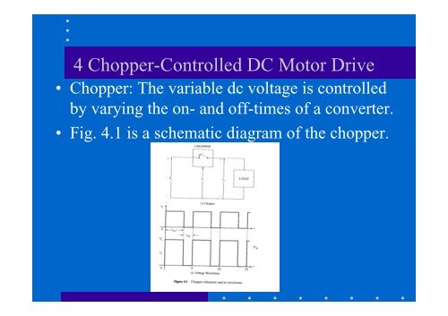
4 Chopper-Controlled DC Motor Drive
4 Chopper-Controlled DC Motor Drive
4 Chopper-Controlled DC Motor Drive

You also want an ePaper? Increase the reach of your titles
YUMPU automatically turns print PDFs into web optimized ePapers that Google loves.
4 <strong>Chopper</strong>-<strong>Controlled</strong> <strong>DC</strong> <strong>Motor</strong> <strong>Drive</strong><br />
• <strong>Chopper</strong>: The variable dc voltage is controlled<br />
by varying the on- and off-times of a converter.<br />
• Fig. 4.1 is a schematic diagram of the chopper.
• Its frequency of operation is<br />
f<br />
1<br />
+ t<br />
c =<br />
=<br />
(ton<br />
off )<br />
1<br />
T<br />
and its duty cycle is defined as<br />
d<br />
=<br />
t<br />
T<br />
on<br />
• Assuming that the switch is ideal, the<br />
average output is<br />
t<br />
V<br />
on<br />
dc = Vs<br />
=<br />
T<br />
dV<br />
s<br />
• varying the duty cycle changes the output<br />
voltage.
• The duty cycle d can be changed in two ways:<br />
(i) varying the on-time (constant switching<br />
frequency).<br />
(ii) varying the chopping frequency.<br />
• Constant switching frequency has many<br />
advantages in practice.
4.3 Four-Quadrant <strong>Chopper</strong> Circuit<br />
• Fig. 4.2 is the chopper circuit with transistor<br />
switches.
• Fig. 4.3 is first-quadrant operation.
• Fig. 4.4 is first-quadrant operation with zero<br />
voltage across the load.
• Fig. 4.5 voltage and current waveforms in<br />
first-quadrant operation.
• Fig. 4.6 second-quadrant operation
• Fig. 4.7 voltage and current waveforms in<br />
second-quadrant operation.
• Fig. 4.8 Modes of operation in the third<br />
quadrant.
• Fig. 4.9 waveform in third-quadrant operation
• Fig. 4.10 Waveforms in fourth-quadrant<br />
operation.
4.4 <strong>Chopper</strong> for inversion<br />
• Converter: <strong>DC</strong> ⇒ <strong>DC</strong> (different voltage)<br />
• The chopper is the building block for that:<br />
AC ⇒ <strong>DC</strong> ⇒ <strong>DC</strong>(different voltage)
4.5 <strong>Chopper</strong> with other power devices<br />
• MOSFETs, IGBTs, GTOs, or SCRs are<br />
used for different power level.<br />
• The MOSFET and transistor choppers are<br />
used at power levels up to 50kW.
4.6 Model of The <strong>Chopper</strong><br />
• The transfer function of the chopper is<br />
G<br />
r<br />
K<br />
(s) =<br />
r<br />
sT<br />
1+<br />
2<br />
where K r = V s /V cm , V s is the source voltage,<br />
and V cm is the maximum control voltage.<br />
• Increasing the chopping frequency decreases<br />
the delay time, and its becomes a simple gain.
4.7 Input to the chopper<br />
• The chopper input: a battery or a rectified ac<br />
supply.<br />
• Fig. 4.11 is the chopper with rectified circuit.
• Its disadvantage: it cannot transfer power from<br />
dc link into ac mains.<br />
• Fig. 4.12 <strong>Chopper</strong> with regeneration capability
• The generating converter has to be operated<br />
at triggering angles greater that 90.
4.8 Other <strong>Chopper</strong> Circuits<br />
• Fig. 4.13 one- and two-quadrant operation.
4.9 Steady-state analysis ...<br />
• 4.9.1 Analysis by averaging<br />
• The average armature current is<br />
I<br />
av<br />
Vdc<br />
− E<br />
=<br />
R<br />
a<br />
where V dc = dV s<br />
• The electromagnetic torque is<br />
T av = K b I av = K b (dV s -K b w m )/R a (N·m)
• The normalized torque is<br />
T<br />
en<br />
=<br />
T<br />
T<br />
av<br />
b<br />
/ V<br />
/ V<br />
b<br />
b<br />
=<br />
K<br />
b<br />
(dV<br />
K<br />
s<br />
b<br />
− K<br />
I R<br />
b<br />
a<br />
b<br />
ωm<br />
) /<br />
/ V<br />
b<br />
V<br />
b<br />
=<br />
dVn<br />
− ω<br />
R<br />
an<br />
mn<br />
,<br />
p.u.<br />
I<br />
R<br />
where R<br />
b a<br />
an = , p.u. V<br />
s<br />
V<br />
n = , p.u. ω<br />
m<br />
mn = , p.u.<br />
b<br />
Vb<br />
ωb<br />
• 4.9.2 Instantaneous steady-state computation<br />
(including harmonics)<br />
• The equations of the motor for on and off times<br />
(continuous current conduction)<br />
di<br />
V E R i L<br />
a<br />
s = + a a + a<br />
dt<br />
di<br />
0 = E + R i L<br />
a<br />
a a + a ,<br />
dt<br />
,<br />
0<br />
dT<br />
≤<br />
≤<br />
t<br />
t<br />
V<br />
≤<br />
≤<br />
dT<br />
T<br />
ω
• Fig. 4.15 The waveform of applied voltage<br />
and armature current.
• The solutions of the above equations:<br />
t<br />
V E<br />
i (t)<br />
s − T<br />
(1 e a T<br />
) I e a<br />
a = − + a0 , 0 < t <<br />
R<br />
i<br />
a<br />
(t)<br />
= −<br />
a<br />
E<br />
R<br />
a<br />
(1 − e<br />
−<br />
1<br />
t<br />
−<br />
T<br />
a<br />
) +<br />
I<br />
a1<br />
e<br />
where T a = L a /R a (Armature time constant)<br />
t 1 = t - dT<br />
• By using boundary condition<br />
I<br />
a1<br />
=<br />
V (1 − e<br />
s<br />
R<br />
a<br />
(1 − e<br />
−dT / T<br />
−T / T<br />
a<br />
a<br />
)<br />
)<br />
−<br />
E<br />
R<br />
−<br />
1<br />
t<br />
−<br />
T<br />
a<br />
a<br />
t<br />
,<br />
I<br />
dT<br />
a0<br />
≤<br />
=<br />
t<br />
≤<br />
V (e<br />
s<br />
R<br />
a<br />
dT<br />
dT<br />
(e<br />
dT / T<br />
T / T<br />
a<br />
a<br />
−1)<br />
−1)<br />
−<br />
E<br />
R<br />
a
• The critical duty cycle: the limiting or<br />
minimum value of duty cycle for<br />
continuous current; I a0 equates to zero.<br />
• The relevant equations for discontinuous<br />
current-conduction mode<br />
V<br />
s<br />
=<br />
E<br />
+<br />
R<br />
a<br />
i<br />
a<br />
+<br />
L<br />
di<br />
dt<br />
di<br />
0 = E + R i L<br />
a<br />
a + a , dT ≤ t ≤ tx<br />
dt<br />
with i a (t x + dT) = 0; i a (0) = 0<br />
a<br />
a<br />
,<br />
0<br />
≤<br />
t<br />
≤<br />
a +<br />
dT<br />
dT
• Hence,<br />
i<br />
a<br />
I<br />
a1<br />
(t<br />
x<br />
=<br />
Vs<br />
−<br />
R<br />
a<br />
+ dT) = −<br />
E<br />
(1 − e<br />
E<br />
R<br />
a<br />
−dT /<br />
(1 − e<br />
Ta<br />
t<br />
−<br />
T<br />
x<br />
a<br />
)<br />
) +<br />
• tx is evaluated from (4.25) and the above<br />
eqs. as<br />
tx = Ta<br />
loge[1<br />
+<br />
I<br />
a1<br />
R<br />
E<br />
a<br />
]<br />
I<br />
a1<br />
e<br />
t<br />
−<br />
T<br />
x<br />
a
• The solution for the armature current in<br />
three time segments is<br />
V E<br />
i (t)<br />
s −<br />
(1 e a<br />
a = − ), 0 < t <<br />
R<br />
i<br />
a<br />
(t)<br />
=<br />
I<br />
a1<br />
e<br />
a<br />
(t−dT)<br />
−<br />
T<br />
a<br />
−<br />
−<br />
t<br />
T<br />
E<br />
R<br />
a<br />
(1 − e<br />
dT<br />
(t−dT)<br />
−<br />
T<br />
ia (t) = 0, (tx<br />
+ dT) < t <<br />
a<br />
),<br />
T<br />
dT<br />
≤<br />
t<br />
≤<br />
t<br />
x<br />
- dT
4.10 Rating of the device<br />
• The rms value of the power switch current<br />
I<br />
t<br />
=<br />
2<br />
max<br />
I<br />
2T<br />
(T + dT) =<br />
1+<br />
d<br />
2<br />
max<br />
• The average diode current<br />
I<br />
1−<br />
d<br />
= ( ) ⋅<br />
2<br />
d I max<br />
⋅ I
• Transistor and diode currents for motoring<br />
operation in the continuous-conduction mode.
4.11 Pulsating Torque<br />
• The average of the harmonic torque is zero.<br />
• High-performance applications require the<br />
pulsating torque to be minimum.<br />
• The applied voltage is resolved into Fourier<br />
components as<br />
V<br />
where<br />
= V +<br />
∞ a ∑ n=1<br />
A<br />
sin(nω<br />
a (t)<br />
n c t n )<br />
dT<br />
V a = Vs<br />
= dV<br />
T<br />
A<br />
n<br />
2V<br />
=<br />
s<br />
nπ<br />
s<br />
nω<br />
dT<br />
sin<br />
c<br />
2<br />
ω<br />
θ<br />
c<br />
n<br />
2π<br />
= 2πf<br />
c =<br />
T<br />
π nωcdT<br />
= −<br />
2 2<br />
+<br />
θ
• The armature current is expressed as<br />
i<br />
a<br />
A<br />
(t) = I<br />
n<br />
av +<br />
∞<br />
∑n<br />
= 1 sin(nωct<br />
+ θn<br />
− φ<br />
Zn<br />
Va<br />
− E<br />
Iav<br />
Zn<br />
= R<br />
Ra<br />
−1<br />
R<br />
φ cos {<br />
a<br />
n =<br />
}<br />
2 2 2<br />
R + n ω L<br />
where<br />
= a c a<br />
a<br />
c<br />
2<br />
a<br />
n<br />
)<br />
+<br />
jnω<br />
L<br />
• The input power is<br />
P<br />
i<br />
=<br />
V<br />
a<br />
⎧V aI<br />
⎪<br />
= ⎨<br />
⎪+<br />
V<br />
⎩<br />
a<br />
(t)i<br />
av<br />
a<br />
+ I<br />
(t)<br />
av<br />
∑<br />
∞<br />
n = 1<br />
sin(nω<br />
t + θ<br />
∞ An<br />
∑ = ω + θ − φ +<br />
∞<br />
n 1 sin(n ct<br />
n n)<br />
∑n<br />
=<br />
Z<br />
n<br />
A<br />
n<br />
c<br />
n<br />
)<br />
1<br />
A<br />
(<br />
Z<br />
2<br />
n<br />
n<br />
sin(nω<br />
c<br />
t + θ<br />
n<br />
)sin(nω<br />
c<br />
t + θ<br />
n<br />
− φ<br />
n<br />
⎫<br />
⎪<br />
⎬<br />
)) ⎪<br />
⎭
4.12 Closed-loop operation<br />
• Fig. 4.20 is the closed-loop speed-controller<br />
dc motor drive.
• The current controller can be<br />
(i) Pulse-Width-Modulation (PWM) controller<br />
(ii) Hysteresis controller<br />
Fig. 4.21 shows on- and off-time for PWM
• Fig. 4.22 is the implementation of PWM<br />
current controller.
• Fig. 4.24 shows hysteresis-controlled operation<br />
a<br />
*<br />
a<br />
i ≤ i − ∆i,<br />
set v =<br />
*<br />
a<br />
a<br />
V<br />
i a ≥ i + ∆i,<br />
reset va<br />
=<br />
s<br />
0
• Fig. 4.23
• Fig. 4.25 is realization of hysteresis controller.