Universität Karlsruhe (TH) - am Institut für Baustatik

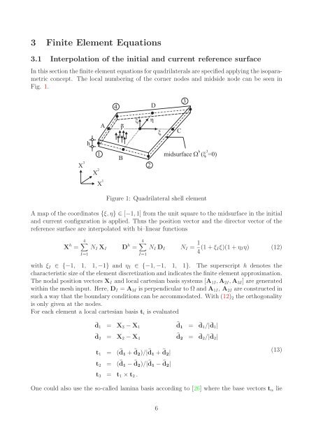
3 Finite Element Equations
3.1 Interpolation of the initial and current reference surface
In this section the finite element equations for quadrilaterals are specified applying the isoparametric
concept. The local numbering of the corner nodes and midside node can be seen in
Fig. 1.
4
D
3
X 3
h
A p
3
C
h
1 midsurface ( =0)
B
2
X 2 X 1 Figure 1: Quadrilateral shell element
A map of the coordinates {ξ,η} ∈[−1, 1] from the unit square to the midsurface in the initial
and current configuration is applied. Thus the position vector and the director vector of the
reference surface are interpolated with bi–linear functions
4∑
4∑
X h = N I X I D h = N I D I N I = 1
I=1
I=1
4 (1 + ξ Iξ)(1 + η I η) (12)
with ξ I ∈ {−1, 1, 1, −1} and η I ∈ {−1, −1, 1, 1}. The superscript h denotes the
characteristic size of the element discretization and indicates the finite element approximation.
The nodal position vectors X I and local cartesian basis systems [A 1I , A 2I , A 3I ] are generated
within the mesh input. Here, D I = A 3I is perpendicular to Ω and A 1I , A 2I are constructed in
such a way that the boundary conditions can be accommodated. With (12) 2 the orthogonality
is only given at the nodes.
For each element a local cartesian basis t i is evaluated
¯d 1 = X 3 − X 1 ̂d 1 = ¯d 1 /|¯d 1 |
¯d 2 = X 2 − X 4 ̂d 2 = ¯d 2 /|¯d 2 |
t 1 = (̂d 1 + ̂d 2 )/|̂d 1 + ̂d 2 |
t 2 = (̂d 1 − ̂d 2 )/|̂d 1 − ̂d 2 |
t 3 = t 1 × t 2 .
(13)
One could also use the so-called lamina basis according to [26] where the base vectors t α lie
6