Lecture 3: Vegetation Sampling - Alaska Geobotany Center
Lecture 3: Vegetation Sampling - Alaska Geobotany Center
Lecture 3: Vegetation Sampling - Alaska Geobotany Center

You also want an ePaper? Increase the reach of your titles
YUMPU automatically turns print PDFs into web optimized ePapers that Google loves.
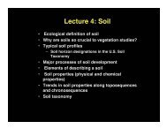
Oct 17 schedule <br />
• 1 hour to go over PCQ lab to see if we can <br />
arrive at the right numbers for density, <br />
frequency, basal area for both transects. <br />
• Short discussion of notebooks. <br />
• <strong>Lecture</strong> on vegeta@on sampling methods.
<strong>Lecture</strong> 3: Vegeta4on <strong>Sampling</strong> <br />
• Subjec4ve vs. objec4ve sampling <br />
• Centralized replicate, random, and systema4c <br />
sampling approaches <br />
• Review of relevé approach <br />
• Cover <br />
• Frequency <br />
• Density <br />
• Tree height <br />
• Biomass and various related indices (LAI, NDVI)
Subjec4ve vs. objec4ve sampling <br />
Subjec've sampling <br />
– Sample sites are consciously chosen as representa4ve of predetermined <br />
vegeta4on classes. <br />
– Most flexible sampling scheme <br />
– Allows for experience and decision making ability of the inves4gator <br />
– Best used in areas where there are clear boundaries between plant <br />
communi4es <br />
– Good approach for vegeta4on classifica4on <br />
Objec've sampling <br />
– Sample sites are chosen according to chance (i.e. random sampling) <br />
– Essen4al if probability sta4s4cs are to be used to back up the <br />
conclusions <br />
– Best used in areas where boundaries between communi4es are <br />
indis4nct or where the objec4ve is to determine the causes of varia4on <br />
within a single plant community <br />
– Good approach for ordina4on methods
Objective sampling approaches<br />
Random <br />
Systema4c <br />
Non stra4fied <br />
Stra4fied
Objec4ve sampling approaches: <br />
Random, and systema4c <br />
Random: Sample sites are chosen according some randomizing method <br />
(e.g., dice, random numbers). Any point is a possible sample point. <br />
– Non-‐stra4fied random: plots are chosen completely randomly. <br />
– Stra4fied random: The research areas is first divided into classes <br />
based on some criteria, for example, landscape units (floodplains, <br />
hills, mountains) or mapped vegeta@on units. Sample sites are <br />
then randomly chosen in the various classes. This ensures that the <br />
most common units are not over-‐sampled and the uncommon <br />
units under sampled. The samples are dispersed throughout the <br />
en@re survey area. <br />
Systema4c: Plots are located according to a regular system such as a grid <br />
or regular intervals along a line. <br />
– Sra4fied systema4c approach is similar to the stra@fied random <br />
approach except the sample sites are chosen according to a <br />
systema@c method (grids or linear transects) within each stra@fied <br />
class.
Subjec4ve sampling approach: <br />
Centralized Replicate <br />
Centralized replicate <br />
– Sample sites are centrally located within representa4ve <br />
homogeneous areas of predetermined vegeta4on types. <br />
– <strong>Sampling</strong> is replicated in many similar areas to obtain a large <br />
sample size of similar vegeta4on. <br />
– This method is used in the relevé approach.
Plot sampling: The relevé method <br />
• French term meaning summary, statement, list or catalog. OZen used in <br />
terms of surveys. <br />
• The quickest way to obtain detailed plant-‐community informa4on. <br />
• Main objec4ve is get a complete list of plant species with cover es4mates <br />
from a representa4ve plant community. <br />
• Standardized approach developed in Europe. <br />
• Applica4on has been tradi4onally been for vegeta4on classifica4on in the <br />
European tradi4on, but the method can be applied to vegeta4on surveys <br />
anywhere and ordina4on methods can be applied to the data. <br />
• Does not necessarily involve sampling other components of the site such as <br />
soils and site factors, although these are oZen collected if environmental <br />
gradient analysis is part of the research. <br />
• Subjec4ve sampling (centralized replicate). <br />
• Qualita4ve in the sense that species cover is es4mated instead of measured. <br />
• Quan4ta4ve in the sense that it gives a complete list of species for the plot. <br />
• Much more on the method later.
En44ta4on and sample site requirements of <br />
relevés: <br />
Requirements of a sample site for a relevé <br />
• Should be recognizable as unit that is repeated in other areas of the landscape, i.e. it is <br />
a repea@ng assemblage of species. <br />
• HOMOGENEITY of the vegeta@on canopy, soil, and other site factors. <br />
• Large enough to contain all the species in the community, but small enough to sample <br />
efficiently and not contain other vegeta@on types (minimum area). <br />
The first step: en'ta'on <br />
• The process of subdividing the vegeta4on into recognizable en44es or preliminary <br />
vegeta4on types <br />
• The first groupings should be at the “habitat type level”. (e.g. stream areas, talus slopes, <br />
discrete soil types) recognizable units on aerial photos, obvious physiognomic <br />
differences. <br />
• Start with the largest easiest to recognize units. <br />
• Reconnaissance essen@al (cannot be overemphasized) The beXer your ini@al <br />
knowledge of an area, the beXer will be the subsequent sampling. <br />
• Important to avoid sampling ecotones or breaks between dis@nct communi@es. <br />
• Knowledge of exis@ng literature and experience in other areas help. <br />
• More subtle floris@c differences will become apparent later. <br />
• Itera@ve process that may take several aXempts to perfect descrip@on of the <br />
communi@es.
Desirable quali4es of relevés: <br />
• Homogeneous. <br />
• Representa4ve of <br />
many areas in the <br />
landscape <br />
• Large enough to <br />
contain the great <br />
majority of <br />
species in the <br />
community <br />
Fred Daniéls collec@ng relevé data at Isachsen, Canada. <br />
Photo D.A. Walker
Relevé sites: <br />
Homogeneity of vegeta4on
How would you sample <br />
this landscape?
Plot size <br />
Minimal Area Method
Plot size <br />
Tables based on previous inves4gators experience
The advantage of permanent plots <br />
• For long-‐term studies. Examine changes due to successional processes, climate <br />
change, or disturbance. <br />
• Complete species list can be made by revisi4ng at different 4mes of year. <br />
• Permits collec4on of other types of informa4on that were not collected during <br />
the first visit, for example, spectral informa4on for remote sensing studies, <br />
observa4ons regarding winter snow depth or other more detailed microclimate <br />
informa4on, biomass informa4on, or physiological informa4on for individual <br />
plant species. <br />
Marking the plots: <br />
In some of our studies, we pound 3/4" rebar in the center of the plot and slip a 60"x1" PVC pipe <br />
over the rebar. The pipe is marked with 10-‐cm stripes that can be used for monitoring snow <br />
depth or water depth in aqua4c vegeta4on. The markers are also highly visible for loca4ng <br />
the plots, par4cularly in winter, and provide a scale for photographing the vegeta4on.
Example of a European relevé protocol, header data <br />
• Relevé No., <br />
• Date, <br />
• Loca4on, <br />
• Site descrip4on, <br />
• Habitat descrip4on <br />
• Brief soil descrip4on <br />
• Area of plot <br />
!
Example of a European relevé protocol: species data <br />
Species data: <br />
• Note separate list for <br />
each layer in canopy. <br />
• Cover-‐abundance score (le_ <br />
column, le_ of decimal), Br.-‐Bl. <br />
cover abundance scores. See <br />
next slides. <br />
• Sociability (le_ column, right of <br />
decimal. See next slides. <br />
• Phenological state (middle <br />
column: See next slides. <br />
• Vigor (right column: See next <br />
slides. <br />
Notes: <br />
1. Except for cover-‐abundance, much of <br />
this informa=on is difficult to quan=fy and <br />
has only minimal value for classifica=on or <br />
ordina=on methods. We will record cover-abundance<br />
for species in each layer, but <br />
ignore the other variables. <br />
2. We make voucher collec=ons of all <br />
species in the plot for the record, and to <br />
insure that mistakes in names are not <br />
made.
Strata (canopy layers) <br />
• Separate lists are made for each layer in the plant <br />
canopy. A single species can appear in more than <br />
one layer. <br />
• Tree layer (can be broken into tall trees (T1) and lower strata trees <br />
(T2) <br />
• Shrub layer (low and tall shrubs or break into S1 and S2) <br />
• Herb layer (includes dwarf shrubs, < 40 cm, or break into H1 <br />
(dwarf shrubs) and H2 (herbs) <br />
• Moss layer (includes mosses, lichens, liverworts)
Sociability (rarely recorded) <br />
• Sociability is a measure of the degree of clustering <br />
(contagion) of individuals of a plant species. <br />
– .1 Growing solitary <br />
– .2 Growing in small groups, or in small tussocks <br />
– .3 Growing in small patches, cushions or large tussocks <br />
– .4 Growing in extensive patches, in carpets or broken mats <br />
– .5 Growing in great crowds or extensive mats covering the whole <br />
plot
Vigor (rarely recorded) <br />
• Vigor is a measure of the vitality of the species in the plot. <br />
– Closed solid circle: Well developed, regularly comple@ng life cycle. <br />
– Open circle with center dot: With vegeta@ve produc@on but not <br />
comple@ng life cycle . <br />
– Open circle: Feeble with low vegeta@ve propaga@on, not <br />
comple@ng life cycle.
Phenology (rarely recorded) <br />
• Phenology provides informa@on regarding the <br />
reproduc@ve status of the plant (v. vegeta@ve, fl. <br />
flowering, fr. frui@ng, s. senescing.).
Site-‐factor data form
Soils <br />
• The soil-‐vegeta@on rela@onships are a key to understanding <br />
vegeta@on paXerns. <br />
• If you have a background in soils, then it is desirable to obtain <br />
as complete soil informa@on from each sample site as <br />
possible. Or work in conjuc@on with a soil scien@st. <br />
• The effort should include digging a soil pit, making a quick <br />
descrip@on of the soil (see relevé soil form), and collec@ng soil <br />
from each soil horizon for later analysis. <br />
• Use a can of known volume to carefully collect the soil. At a <br />
minimum, a grab sample (large handful) of soil should be <br />
obtained from the top mineral horizon (generally 10 cm <br />
depth). This can later be analyzed for pH, percent soil <br />
moisture, soil texture, soil color, percent organic maXer, soil <br />
nutrients (N, P, K) and other physical and chemical <br />
characteris@cs. <br />
• In our class sampling, we use a simplified soil descrip=on that <br />
is part of the site factor data sheet, and we will collect soil <br />
samples from the roo=ng zone (about 10 cm) or the top of the <br />
first mineral horizon in organic-‐rich (peaty) soils.
Soil descrip4on form (for those with experience <br />
in soils descrip4on)
Photographs <br />
• Photographs can be extremely valuable for later reference. <br />
• We generally take at least three photographs: <br />
(1) the loca4on of the plot within the general landscape, preferably <br />
with a stake marked with the plot number in the center of the plot; <br />
(2) one or more ver4cal close-‐ups of the vegeta4on; and <br />
(3) a photo of the soil profile that includes a label giving the plot <br />
number, a ruled tape for scale, and markers (e.g. nails) that <br />
delineate the boundaries between the soil horizons.
Cover <br />
The area of ground covered by the ver4cal projec4on of the <br />
aerial parts of plants of one or more species. <br />
• An easily obtained index of plant biomass. <br />
• The variable most oZen recorded.
Es4mates vs. measures of cover <br />
• Es4mates of cover can be obtained by using cover-‐abundance <br />
scores. Most useful for classifica@on. <br />
• Measures of cover can be made using point sampling <br />
methods, line transect method, or photos and planimeter or <br />
other direct measure of cover. O_en necessary for change <br />
analysis and more quan@ta@ve studies.
Es4ma4ng percentage cover <br />
• Generally a ball-‐park es4mate is good enough <br />
(e.g., 20% for species B above. This falls in B-‐B <br />
cover-‐abundance category 3, which is the same <br />
as the actual cover (33%) determined by <br />
measurement.) <br />
• Cover is very difficult to <br />
accurately es4mate. The <br />
use of cover-‐abundance <br />
scores greatly reduces <br />
the varia4on in scores <br />
from observer to <br />
observer. <br />
• For the relevé method, <br />
actual scores are not as <br />
important as the <br />
presence or absence of <br />
species. <br />
• Cover is a secondary <br />
considera4on in the <br />
Braun-‐Blanquet table <br />
analysis method.
Cover-‐abundance classes
Measuring Cover: <br />
Line intercept method <br />
• Generally used for tree and shrub cover or for measuring cover of <br />
clearly defined vegeta4on types <br />
• A line is laid out along the ground and the line segments for each <br />
species or vegeta4on type is recorded. <br />
• Percentage cover for each species is the total length of line <br />
segments for each species divided by the total length of the <br />
transect.
Measuring Cover: <br />
Point intercept methods <br />
• Many methods <br />
– Point quadrats <br />
– Point frames <br />
• Ver4cal point frames <br />
• Inclined point frames <br />
– Moosehorn crown cover es4mator <br />
– Laser points <br />
– Op4cal point sampling devices
Advantages and disadvantages of point-intercept<br />
methods <br />
• Advantages <br />
– objec@ve <br />
– confidence in values (accurate & precise) <br />
– repeatable <br />
• Disadvantages <br />
– @me consuming <br />
– emphasizes most common plants <br />
“best suited to applica=ons such as mine permit baselines and tes=ng for <br />
revegeta=on success, where maximum confidence in absolute cover and <br />
repeatability is paramount and informa=on on the full range of individual <br />
species' cover values is not.” (Buckner web site)
Ver4cal point frame <br />
Martha Raynolds
Point methods <br />
Sloping point frame to <br />
32.5% makes it least <br />
affected by foliage <br />
angle. Will increase <br />
values, but may provide <br />
beXer comparison <br />
between stands in some <br />
vegeta@on types. <br />
% cover<br />
Effect of point diameter: Ideal is infinitely small <br />
Percent cover measured by 100 pins<br />
100<br />
80<br />
60<br />
grass FESRUB<br />
40<br />
forb RANACR<br />
moss HYLSPL<br />
20<br />
0<br />
0 1 2 3 4 5 6<br />
Diameter of pin (mm)<br />
Shimwell 1972 <br />
• First hit is always recorded <br />
• Successive hits on same species recorded if interested in leaf area <br />
• Hits of other layers o_en recorded <br />
• Understory hit (usually moss layer) o_en recorded <br />
• Height can be recorded <br />
• Various liXer and bare categories can be defined
Point quadrat
Point quadrat grid
Point quadrat grid <br />
Walker, D.A., Walker, M.D., Gould, W.A., Mercado, J., Auerbach, N.A., Maier, H.A., Neufeld, G.P. 2010. Maps for monitoring changes to<br />
vegetation structure and composition: The Toolik and Imnavait Creek grid plots. Viten. 1:121-123.
Point quadrat grid <br />
Walker, D.A., Walker, M.D., Gould, W.A., Mercado, J., Auerbach, N.A., Maier, H.A., Neufeld, G.P. 2010. Maps for<br />
monitoring changes to vegetation structure and composition: The Toolik and Imnavait Creek grid plots. Viten. 1:121-123.
Point quadrat grid <br />
Walker, D.A., Walker, M.D., Gould, W.A., Mercado, J., Auerbach, N.A., Maier, H.A., Neufeld, G.P. 2010. Maps for<br />
monitoring changes to vegetation structure and composition: The Toolik and Imnavait Creek grid plots. Viten. 1:121-123.
Time-‐series results from Imnavait Creek <br />
point-‐quadrat data <br />
Data from W.G. Gould and J. Mercado.
Funky methods of determining tree-‐canopy cover <br />
Densitometer with single cross hairs <br />
Moosehorn crown-cover estimator <br />
Spherical densiometer
Buckner sampler: Op4cal Sigh4ng Device (OSD)
Basal area <br />
• A measure of dominance. Generally used for trees. <br />
• The cross-‐sec4onal area of tree stems at breast height per <br />
unit of ground area (e.g., m 2 /ha) <br />
• Methods of determining basal area <br />
– Measure tree diameters at breast height with a biltmore s4ck or <br />
diameter tape. Area = π(dbh/2) 2 . This approach is used in count-‐plot <br />
and distance methods (e.g., point-‐centered quarter method). <br />
– Bijerlich s4ck, or angle gauge <br />
• We will discuss basal area more thoroughly when we discuss <br />
methods of measuring density and dominance of forest <br />
species (point-‐centered quarter method and count-‐plot <br />
method).
Frequency <br />
• Expressed as a percentage of plots (quadrats) of <br />
equal size in which at least one individual of the <br />
species occurs in a group of plots. <br />
• It is a measure of the degree of uniformity with <br />
which individuals of a species are distributed in a <br />
vegeta4on type.
Density <br />
• The number of plants per unit area. Expressed as number/<br />
square meter, stems/acre, etc. <br />
• Most oZen used for trees or large plants. <br />
• An an easy concept to grasp, but very difficult to perform in <br />
some types of vegeta4on because of: <br />
(1) the difficulty of defining an individual (e.g. caespitose growth forms, <br />
plants with underground rhizomes, plants in peaty landscapes oZen <br />
have complicated stems just beneath the surface of the moss layer) <br />
(2) quadrat size affects density size because of problem of coun4ng <br />
large individuals near the boundary of the quadrat <br />
(3) it is very 4me-‐consuming in graminoid dominated systems and low-growing<br />
vegeta4on, or moss or lichen communi4es.
Tree height <br />
Use your trigonometry <br />
for something useful! <br />
There are many <br />
methods. We will use <br />
one: <br />
45 o 90 o <br />
45 o <br />
1 2 <br />
• If the tree is ver4cal, and you stand <br />
where the angle to the top of the tree is 45 <br />
degrees, the distance from you to the tree <br />
is the same as its height <br />
• To get the angle to be 45 degrees <br />
• measure the length of your arm, <br />
from shoulder to fist <br />
• hold the meter s4ck ver4cally, so <br />
that distance extends above your fist <br />
• if you put your eye close to your <br />
shoulder and sight at the top of the <br />
meter s4ck, that is 45 degrees <br />
• walk to a point where you can sight <br />
on the top of the tree and are level <br />
with the bojom <br />
• measure the distance to the bojom <br />
of the tree <br />
1
Tree height
Biomass (phytomass) <br />
• Total standing crop (g m -‐2 ) <br />
• Clip harvest <br />
– usually sorted into categories such as live vs. dead, plant <br />
func@onal types, etc. <br />
– dried and weighed <br />
– (can be frozen before these steps)
Biomass clip harvest<br />
1 2<br />
3<br />
4<br />
5<br />
6<br />
7<br />
8
Biomass sor4ng according plant func4onal <br />
types
Plant func4onal type sor4ng categories <br />
• Deciduous shrubs<br />
– Woody stems<br />
– Foliar<br />
• Live<br />
• Dead<br />
• Evergreen shrubs<br />
– Woody stems<br />
– Foliar<br />
• Live<br />
• Dead<br />
• Forbs<br />
• Live<br />
• Dead<br />
• Graminoids<br />
• Live<br />
• Dead<br />
• Lichens<br />
• Live<br />
• Dead<br />
• Mosses<br />
• Live<br />
• Litter<br />
• Dead
Methods of measuring biomass or <br />
proper4es that are surrogates of biomass <br />
• Aboveground biomass <br />
– Clip harvest <br />
– Dimension analysis <br />
• Belowground biomass <br />
– Soil cores <br />
– In situ root washing <br />
– Root ingrowth bags <br />
– Mini-‐rhizotrons (root length, root produc@on, death) <br />
• Leaf area index (LAI) <br />
– Point frame <br />
– Li-‐COR instruments <br />
• Remote sensing vegeta4on indices <br />
– Normalized difference vegeta@on index (NDVI)
Clip Harvest <br />
• Normally, several small representa@ve areas (e.g. 0.1 m 2 <br />
for graminoid communi@es) are clipped. <br />
• Normally it is desirable to provide more detail from clip <br />
harvests than total mass per unit area. <br />
• Sor@ng of the harvest can be by any of several criteria, or <br />
combina@on thereof, for example: <br />
1. Species <br />
2. Growth forms <br />
3. Live vs. dead <br />
4. Foliar vs. woody (useful for determining green biomass) <br />
5. Plant parts (flowers, stems, leaves, seeds, etc.). <br />
• Once sorted, the components are oven dried (105° C) and <br />
weighed, and biomass expressed as mass/unit area
<strong>Alaska</strong> Tundra Biomass Sor4ng <br />
Forbs Graminoids Dwarf Shrubs Horsetails Mosses Lichens <br />
Live Dead Live Dead Live Dead <br />
Evergreen Deciduous <br />
Woody Foliar Woody Foliar <br />
Live Dead <br />
Live Dead
Biomass sampling in forests <br />
dbh
Belowground biomass <br />
• Below ground harvest <br />
– Much more difficult to obtain. <br />
– In herbaceous vegeta@on several cores are take by taken by pressing a coring tube <br />
(e.g., 10-‐cm diameter) into the soil and extrac@ng soil containing roots. <br />
– The cores are washed to remove the soil. <br />
– Live from dead roots can some@mes be determined by color of the roots, or <br />
applica@on of tetrazolium salts. <br />
– Woody root systems may require excava@on and exposure of the root system in <br />
situ. <br />
• Root ingrowth bags <br />
– Numerous small nylon mesh bags of known diameter and volume are filled with <br />
soil and inserted into the ground. <br />
– These are retrieved at intervals, and the ingrown roots are removed and weighed. <br />
• Minirhizotrons <br />
– Photos taken at regular intervals along a tube inserted into the ground. PaXerns of <br />
fine roots are photographed at several @mes during the summer, and root growth <br />
is recorded on video. <br />
– Growth is obtained by taking periodic photos.
Minirhizotron <br />
apparatus <br />
Photo: Roger Ruess
Photo of roots through the minirhizotron apparatus
Net primary produc4vity (NPP) <br />
NPP = (W t+1 -‐ W t ) + D + H <br />
(W t+1 -‐ W t ) = difference in biomass between two <br />
harvests <br />
D = biomass lost to decomposi@on <br />
H = is the biomass lost to herbivory
Leaf Area Index (LAI) <br />
• An index of the ra4o of the area of leaves and green vegeta4on in <br />
the plant canopy per unit area of ground surface <br />
• LAI is a nondestruc4ve, rela4vely fast method of obtaining an <br />
es4mate of biomass. <br />
• The only way to get true leaf area is to strip all the leaves off the <br />
plants and measure their area. <br />
• All other methods provide an “index” of this value (e.g. inclined <br />
point frame, LICOR-‐2000). <br />
• Regression methods are used to relate biomass to leaf area.
Inclined point frame <br />
32.5˚ @lt was <br />
determined as the <br />
best compromise for <br />
determining the area <br />
of leaves in mixed <br />
canopies of <br />
erectophyllic and <br />
planophyllic leaves.
Electronic inclined point frame for <br />
determining LAI
Li-COR® LAI-2200 Plant Canopy Analyzer<br />
• Very rapid method of <br />
obtaining field LAI. <br />
• Provides only total LAI, and <br />
cannot dis4nguish <br />
components of individual <br />
species nor of woody vs. <br />
foliar frac4on. <br />
• Not useful for very low <br />
growing vegeta4on (moss <br />
and lichen mats) because the <br />
height of the sensor is above <br />
most moss and lichens (about <br />
2.5 cm). <br />
Courtesy of Li-‐COR Biosciences
• Reference <br />
reading is taken <br />
above the plant <br />
canopy. <br />
• Below the canopy <br />
measurement is <br />
then taken and <br />
the instrument <br />
records the <br />
difference in the <br />
two readings of <br />
light as the LAI.
Source: Li-COR manual <br />
Correla4on between actual leaf area <br />
and LAI measured with the LAI-‐2000
Normalized Difference Vegeta4on <br />
Index (NDVI) <br />
• One of several spectral vegeta4on indices that use <br />
reflectance in variance bands of the total spectrum to <br />
determine and index of vegeta4ve abundance. <br />
• The NDVI is based on the principle that red, R, wavelengths <br />
(near 0.6µm) are absorbed by chloroplasts and mesophyll, <br />
while near infrared, NIR, wavelengths (0.7-‐0.9µm) are <br />
reflected.
Energy inputs to the top of the Earth’s atmosphere and surface <br />
Top of Atmosphere <br />
Percent reaching Earth Surface <br />
From Lillisand and Kiefer 1987
Reflectance spectra for typical components <br />
of the Earth’s surface <br />
From Lillisand and Kiefer 1987
Different vegeta4on types have different <br />
reflectance spectra depending mainly on chlorophyll content
Absorption spectra<br />
for different plant<br />
pigments and<br />
photosynthetic<br />
response<br />
• The pigments in plant<br />
leaves, chlorophyll,<br />
strongly absorbs visible<br />
light (from 0.4 to 0.7 µm).<br />
for use in photosynthesis.
Some reflectance spectra <br />
The cell structure of the <br />
leaves and the plant canopy, <br />
strongly scajer near-‐infrared <br />
light (from 0.7 to 1.1 µm). <br />
(http://internet1-ci.cst.cnes.fr:8100/cdrom/ceos1/titlep.htm)<br />
Normalized Difference Vegeta4on Index, NDVI = (NIR – R) / (NIR + R)
The difference in the <br />
reflectance in the NIR and <br />
red regions is the numerator <br />
of the NDVI. <br />
The sum of these <br />
reflectances is the numerator <br />
which normalizes the value <br />
and corrects for shadows and <br />
different slope aspects. <br />
(http://internet1-ci.cst.cnes.fr:8100/cdrom/ceos1/titlep.htm)<br />
Normalized Difference <strong>Vegetation</strong> Index, NDVI = (NIR – R) / (NIR + R)
Satellites measure reflectance in discreet bands or channels <br />
From Lillisand and Kiefer 1987
Thema@c Mapper (TM) Sensor bands on Landsat 4 and 5 satellites
Normalized Difference Vegeta4on Index: an <br />
index of greenness <br />
NDVI = (NIR-‐R)/(NIR+R) <br />
NIR = spectral reflectance in the near-‐infrared band <br />
(0.725 -‐ 1.1µm), where light scaXering from the canopy <br />
dominates, <br />
R = reflectance in the red, chlorophyll-‐absorbing por@on <br />
of the spectrum (0.58 to 0.68µm).
Hand-held spectroradiometer for ground-level<br />
measurement of spectral reflectance<br />
• There are several <br />
brands of hand-‐held <br />
radiometers that <br />
mimic the sensors in <br />
satellites. <br />
• Some have four <br />
sensors that can be <br />
set to sense the same <br />
band widths as <br />
common satellite <br />
sensors. <br />
• Most of the newer <br />
ones have large <br />
numbers of channels <br />
(ASD instruments <br />
have 256 channels). <br />
Courtesy of Analy@cal Spectral Devised, Inc., Boulder, CO
Biomass and LAI vs. <br />
total summer <br />
warmth index <br />
1200<br />
1000<br />
800<br />
600<br />
Above-ground biomass vs. Total summer<br />
warmth<br />
Biomass <br />
y = 85.625e 0.0703x<br />
R 2 = 0.9131<br />
Oumalik<br />
Ivotuk<br />
MAT<br />
MNT<br />
400<br />
200<br />
Barrow<br />
Atqasuk<br />
Oumalik<br />
Ivotuk<br />
0<br />
0 10 20 30 40<br />
Total Summer Warmth<br />
( o C)<br />
Leaf Area Index vs. Total Summer Warmth<br />
Leaf Area Index (LAI) <br />
3<br />
2.5<br />
2<br />
y = 0.4763e 0.0463x<br />
R 2 = 0.933<br />
Ivotuk<br />
MAT<br />
MNT<br />
1.5<br />
Oumalik<br />
1<br />
0.5<br />
Barrow<br />
Atqasuk<br />
Ivotuk<br />
Oumalik<br />
0<br />
0 10 20 30 40<br />
Total Summer Warmth<br />
( o C)
NDVI vs. total aboveground biomass <br />
NDVI vs. Total Biomass<br />
0.6<br />
0.55<br />
0.5<br />
y = 0.0005x + 0.1471<br />
R 2 = 0.9827<br />
Oumalik<br />
Ivotuk<br />
0.45<br />
0.4<br />
Barrow<br />
0.35<br />
Atqasuk<br />
0.3<br />
200 300 400 500 600 700 800<br />
TotalBiomass (g/m 2 )
AVHRR false-‐Color infrared mosaic <br />
Redder areas <br />
have more <br />
biomass
MaxNDVI map of the circumpolar Arc4c <br />
MaxNDVI <br />
0.62
Eurasia Arctic Transect<br />
Plot-level biomass trends<br />
along two North-South<br />
Arctic Transect<br />
North America Arctic Transect<br />
83
Arc4c phytomass based on NDVI data from <br />
clip harvests