Internal generation of waves for extended Boussinesq equations

Ž .
Coastal Engineering 42 2001 155–162
www.elsevier.comrlocatercoastaleng
Internal generation of waves for extended Boussinesq equations
Changhoon Lee a,) , Yong-Sik Cho b , Kidai Yum c
a Department of CiÕil and EnÕironmental Engineering, Sejong UniÕersity, 98 Kunja-dong, Kwangjin-ku, Seoul, 143-747, South Korea
b Department of CiÕil Engineering, Hanyang UniÕersity, 17 Haengdang-dong, Songdong-ku, Seoul 133-791, South Korea
c Coastal and Harbor Engineering Research Center, Korea Ocean Research and DeÕelopment Institute, Ansan P.O. Box 29,
Seoul 425-600, South Korea
Received 13 August 1999; received in revised form 17 August 2000; accepted 12 September 2000
Abstract
It is studied whether the mass transport or energy transport is the proper viewpoint for internally generating waves in the
extended Boussinesq equations of Nwogu wJ. Waterw., Port, Coastal Ocean Eng. 119 Ž 1993. 618–638 x. Numerical solutions
of the Boussinesq equations with the internal generation of sinusoidal waves show that the energy transport approach yields
the required wave amplitude properly while the mass transport approach yields wave amplitude different from the required
one by the ratio of phase velocity to energy velocity. The waves which pass through the wave generation point do not cause
any numerical distortion while the incident waves are generated. The technique of internal generation of waves shows its
capability of generating nonlinear cnoidal waves as well as linear sinusoidal waves. q 2001 Elsevier Science B.V. All rights
reserved.
Keywords: Extended Boussinesq equations; Internal generation of waves; Mass transport; Energy transport; Numerical test
1. Introduction
The propagation of water waves is a dynamic
phenomenon which gives the human beings happiness
some time or a disaster other time. Identification
of the physical behavior of water waves is still
ongoing research topic. The Boussinesq equations
are known to predict the random and nonlinear behavior
of water waves with high accuracy especially
in shallow water. The equations were developed
firstly by Boussinesq Ž 1872.
for waves over a constant
water depth and later were extended to variable
water depths by Peregrine Ž 1967 .. The Boussinesq
) Corresponding author. Fax: q82-2-3408-3332.
Ž .
E-mail address: clee@sejong.ac.kr C. Lee .
equations, which are composed of the continuity
equation and x- and y-momentum equations, are
derived based on two parameters, the dispersiveness
of the relative water depth kh Žk is the wave number
and h is the water depth.
and the nonlinearity of the
relative wave amplitude arh Ža is the wave amplitude.
and on the assumption of kh

156
( )
C. Lee et al.rCoastal Engineering 42 2001 155–162
superiority of the Boussinesq equations to other wave
equations has been strengthened. Two types of the
extended Boussinesq equations have been developed.
The first type was developed by adding correction
terms to the momentum equations in order to get the
linear dispersion relation close to the exact one
Ž Madsen et al., 1991; Madsen and Sorensen, 1992 ..
The second type was developed by using the horizontal
velocities at a certain level instead of the
depth-averaged velocities in order to get the linear
dispersion relation close to the exact one ŽNwogu,
1993 .. The model of Nwogu, which is accurate to
OŽŽ kh . 2 , arh ., was developed in a different form
with the velocity potential instead of the particle
velocity by Chen and Liu Ž 1995 .. It was extended to
OŽŽ kh . 2 , Ž arh. 3 Ž kh. 2 . by Wei et al. Ž 1995 ., and
further to OŽŽ kh . 4 , Ž arh. 5 Ž kh. 4 . by Madsen and
Schaffer ¨ Ž 1998 .. It was also extended to consider the
case of waves on a current with OŽŽ kh . 2 , arh.
by
Chen et al. Ž 1998 ..
The hyperbolic-type wave equations may be used
to solve a lot of engineering problems such as design
wave height or harbor resonance because the behavior
of water waves is predicted in real time and the
reflection conditions at coastal structures can be
specified at will. The solution process of the hyperbolic-type
wave equations starts with a calm state of
surface elevations and continues until the wave energy,
which is made at offshore boundaries, propagates
to the region of interest. The wave energy
would reflect against the coastal structures and propagate
back to the offshore boundaries. The open
boundary conditions may be specified perfectly if the
wave energy which is reflected back to the offshore
boundaries is transmitted without any re-reflection
back to the computational domain. This is possible
by generating waves internally at a wave generation
line which is placed inside the computational domain
while a sponge layer is placed at offshore boundaries
Ž Larsen and Dancy, 1983 .. Then the wave which is
generated at the wavemaker would propagate in both
directions from the wave generation line and some
wave energy which is reflected against the structure
would pass through the wave generation line without
any numerical distortion, and further be absorbed in
the sponge layer at the offshore boundaries.
There are two different viewpoints related to the
internal wave generation. One is the viewpoint of
mass transport that the water mass which is generated
at the wave generation line transports in phase
velocity. The viewpoint is applied in the Boussinesq
equations of Peregrine Ž Larsen and Dancy, 1983.
and
the mild-slope equations of Copeland Ž 1985. ŽMad-
sen and Larsen, 1987; Yoon et al., 1996 .. The other
is the viewpoint of energy transport that the wave
energy which is generated at the wave generation
line transports in energy velocity. This viewpoint is
applied in the mild-slope equations of Radder and
Dingemans Ž 1985. and Copeland ŽSuh et al., 1997;
Lee and Suh, 1998 .. Lee and Suh found that application
of the mass transport approach to the mild-slope
equations of Radder and Dingemans yields improper
wave energy. They also found that, in the case of
equations of Copeland, two viewpoints of the mass
transport and energy transport give the same results
because the energy velocity is the phase velocity.
Further, they implied that, in the case of equations of
Peregrine, the mass transport approach might be
applied properly because the phase velocity in shallow
water is almost the same as the energy velocity.
In other words, it would be problematic to use the
viewpoint of mass transport in deeper water.
In this study, it will be found whether the mass
transport or energy transport approach yields a proper
wave energy for internally generating waves in the
Boussinesq equations of Nwogu. In Section 2, the
approaches of the mass transport and energy transport
are described and the phase and energy velocities
are derived. In Section 3, in a horizontally
one-dimensional domain, a finite difference method
is used to discretize the equations of Nwogu. Then,
the cnoidal waves and sinusoidal waves are generated
internally with two different approaches. Finally,
concluding remarks are made in Section 4.
2. Mass transport and energy transport
The extended Boussinesq equations of Nwogu
Ž 1993.
are written as:
Eh z 2 a h 2
q=P Ž hqh. u q=P y h= Ž =Pu.
Et 2 6
ž /
½ž /
h
q z q h= =P Ž hu. s0 Ž 1.
2
a 5

( )
C. Lee et al.rCoastal Engineering 42 2001 155–162 157
Eu
q Ž uP= . uqg=h
Et
a½ ž / ž / 5
za
Eu Eu
qz = =P q= =P h s0.
2 Et Et
Ž 2.
In Eqs. Ž. 1 and Ž. 2 , h is the water surface elevation,
u is the horizontal velocity vector at a certain
elevation of zsz a, h is the mean water depth, g is
the gravitational acceleration, = is the horizontal
gradient operator, and asŽ z .
arh 2 r2qzarh. In
this study, asy0.4 is used which gives zarhs
y0.55.
Waves are generated internally by adding the
value of h ) to the computed surface elevation h at
the wave generation line at each time step. The value
of h ) is given by:
° I
CDt
2h cosu , mass transport
) ~ D x
h s , Ž 3.
CeDt
I
¢ 2h cosu , energy transport
D x
where h I is the water surface elevation of incident
waves, C and Ce
are the phase and energy velocities
of incident waves, respectively, u is the angle of
wave rays from the x-axis, D x is the grid size in the
x-axis, and Dt is the time step. The wave generation
line is assumed to be parallel to the y-axis.
The phase velocity and energy velocity of waves
can be obtained analytically using the geometric
optics approach. In the case that water depths are
constant and the nonlinear terms are ignored, differentiating
Eq. Ž. 1 in space, differentiating equation
Eq. Ž. 2 in time, and eliminating h from two resultant
equations yield the following equation as,
E 2 u
ygh= =Pu Ž .
Et 2
ž /
1
y aq
3
Ž . 4
3
gh= =P = =Pu
ž /
E 2 u
2
qa h = =P s0. Ž 4
2
.
Et
When we consider the wave field along the direction
of wave ray, i.e., s-direction, the wave field may
be analyzed in one dimension. Then, the particle
velocity u may be defined as,
usAe ic , Ž 5.
where A is the amplitude of the velocity and the
phase function c has the following relations with
the wave number k and angular frequency v as,
Ec Ec
ks , vsy . Ž 6.
Es Et
Substituting Eq. Ž. 5 into Eq. Ž. 4 and rearranging
the real part of the resultant equation to the order of
OŽ.
1 yield the phase velocity C as:
) ž /
2
1
2
1y aq Ž kh
v
.
3
Cs s gh . Ž 7.
k
1ya Ž kh.
Substituting Eq. Ž. 5 into Eq. Ž. 4 , rearranging the
imaginary part of the resultant equation to the order
of OŽ E ArEt, E ArEs ., and further multiplying by A
yield the transport equation for wave energy given
as,
E A 2 E A 2
qCe
s0, Ž 8.
Et Es
where the energy velocity Ce
is given by:
2
Ž kh.
Ce sC 1y .
1
2 2
3½1yž aq
/ Ž kh. 51ya Ž kh.
4
3
Ž 9.
It should be noted that the energy velocity Ce
is
the same as the group velocity Cg
sEvrEk obtained
by Nwogu Ž 1993 ..
3. Numerical experiment
Numerical experiments are conducted in horizontally
one-dimensional cases. The governing equations
are discretized in time using the predictor-cor-

158
( )
C. Lee et al.rCoastal Engineering 42 2001 155–162
rector scheme. Both cnoidal and sinusoidal waves
are generated internally from two viewpoints of the
mass transport and energy transport.
3.1. Finite difference method
Sponge layers are placed at boundaries in order to
minimize wave reflections from the boundaries. Eqs.
Ž. 1 and Ž. 2 can be written in a horizontally one-dimensional
domain as,
½ž /
Eh E E z 2 a h 2 E 2 u
q Ž hqh. u4
q y h
2
Et Ex Ex 2 6 Ex
ž /
h E 2
q z q h Ž hu. s0 Ž 10.
2 Ex
a 2 5
½ ž / 5
Eu 1 Eu 2 Eh za
E 3 u E 2 Eu
q qg qza q h
2 2
Et 2 Ex Ex 2 Ex Et Ex Et
qv Dus0, s
Ž 11.
where,
° d r S
~ e y1 , inside sponge layer
Ds s ey1
. Ž 12.
¢ 0, outside sponge layer
In Eq. Ž 12 ., Ss2.5 L Ž L is the wavelength.
is the
thickness of the sponge layer and d is the distance
from the starting point of the sponge layer.
The variables h and u in Eqs. Ž 10. and Ž 11.
iy1r2 i
are placed in a staggered grid system where the
subscript i denotes the spatial grid point. The firstorder
spatial derivative terms in Eqs. Ž 10. and Ž 11.
are discretized to OŽŽ D x . 4 .. Both the second-and
third-order spatial derivative terms in Eq. Ž 10.
are
discretized to OŽŽ D x. 2 . and the second-order spatial
derivative terms in Eq. Ž 11.
are discretized to
OŽŽ D x . 4 ..
The time derivative terms in Eqs. Ž 10. and Ž 11.
are discretized to OŽŽ Dt. 2 . using the predictor-corrector
method. Eq. Ž 10.
is discretized explicitly between
the n-th and Ž nq1r2.
-th time steps to get the
p
surface elevation h at the Ž nq1r2.
-th time step.
The superscript p in h stands for the predictor. Eq.
Ž 10.
is discretized again implicitly between the n-th
and Ž nq1r2.
-th time steps to get the surface elevanq1r2
tion h at the Ž nq1r2.
-th time step. At this
time, the surface elevation h and the particle velocity
u in the spatial derivatives are replaced by h p
and Žu n qu nq1 . r2, respectively. And then, Eq. Ž 11.
is discretized between the n-th and Ž nq1.
-th time
steps. At this time, the surface elevation h is replaced
by h nq1r2 . The resulting equation gives a
hepta-diagonal matrix of u nq1 given as:
Au nq1 qBu nq1 qCu nq1 qDu nq1 qEu nq1
i iy3 i iy2 i iy1 i i i iq1
qFiuiq2 nq1 qGu i iq3 nq1 sH i , Ž 13.
where A i, ..., Hi
are coefficients of h n and u n .
Using the method of LU decomposition ŽPress et al.,
1992 ., Eq. Ž 13.
is solved to get the particle velocity
nq1
u . Again, Eq. Ž 10.
is discretized between the n-th
and Ž nq1.
-th time steps. At this time, the particle
velocity u is replaced by Žu n qu nq1 . r2 and the
surface elevation h in EŽ hqh. u4
i
rEx is replaced
Ž
n nq1 n nq1
by h qh qh qh .
iq1r2 iq1r2 iy1r2 iy1r2 r4. The re-
sulting equation gives a penta-diagonal matrix given
as,
ah nq1 qbh nq1 qgh nq1 qdh nq1
i iy5r2 i iy3r2 i iy1r2 i iq1r2
qeihiq3r2 nq1 ss i , Ž 14.
where a i, ..., si
are coefficients of h n , u n , and
u nq1 . Using the method of LU decomposition, Eq.
Ž .
nq1
14 is solved to get the surface elevation h .
Waves are generated smoothly by multiplying
Ž . Ž .
)
tanh nDtrT T is the wave period to h in Eq.
Ž. 3 . At both the left and right boundaries, a reflective
boundary condition is specified as:
u nq1 s0, u nq1 s0, h nq1 sh nq1 ,
1 Iy1 1r2 3r2
h nq1 sh nq1 , Ž 15.
Iy1r2
Iy3r2
where is1 and isIy1 denote the points of the
left and right boundaries, respectively. The grid size
is chosen as D xsLr20 in order to get sufficient
spatial resolution. The time step is chosen so that the
Courant number is CrsCe
DtrD xs0.2 and a sta-
ble solution is guaranteed.

( )
C. Lee et al.rCoastal Engineering 42 2001 155–162 159
3.2. Uni-directional regular waÕes
Firstly, cnoidal waves are generated internally
with the condition of Larsen and Dancy Ž 1983 .. The
computational domain consists of an inner domain of
400 m and a sponge layer at the right boundary. The
wave generation point is located at the mid-point of
the inner computational domain. The wave period is
Ts20 s, the wave height is Hs0.5 m, and the
water depth is hs10 m, which gives the wavelength
Ls195 m, the relative water depth khs
0.1p , the wave steepness arhs0.025, and the
Ursell number U Ž . Ž .
r s arh r kh
2 s0.24. Both the
mass transport and energy transport approaches are
used to generate waves.
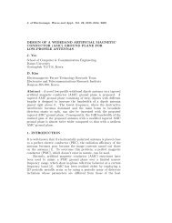
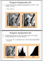
Fig. 1 shows the surface elevations at time between
ts10T and ts11T with an interval of
Tr10. Good agreement is observed between this
figure and Fig. 2 of Larsen and Dancy Ž 1983 .. This
is because, in shallow water with khs0.1p , the
equations of Nwogu Ž 1993.
are almost the same as
those of Peregrine Ž 1967 .. Numerical solutions of the
wave amplitude by the mass transport approach are
3% larger than those by the energy transport approach
which matches the ratio of CrCe
s1.03 for
khs0.1p.
In Fig. 1, the incident waves generated at the
wave generation point propagate both directions
while the waves reflected from the left boundary
pass through the wave generation point with no
serious numerical distortion. Such good work for
internally generating waves wouldn’t be seen if the
unstaggered grid scheme is used in the Boussinesq
equations of Nwogu Ž Wei et al., 1999 .. This is
probably because the unstaggered grid scheme may
result in distortion of the solution. Lee and Suh
Ž 1998.
found that the use of the unstaggered grid
scheme in the time-dependent mild-slope equations
of Radder and Dingemans Ž 1985.
is all right for the
internal wave generation. This is probably because
the model equations are linear and the distortion of
the solution is not serious. However, the resolved
wave height was found to fluctuate around the exact
solution due to the use of the unstaggered grid
Fig. 1. Surface elevations of internally generated cnoidal waves; solid linesenergy transport, dashed linesmass transport.

160
( )
C. Lee et al.rCoastal Engineering 42 2001 155–162
scheme. In the study of Lee and Suh, the phenomenon
of such fluctuations is not observed for the
equations of Copeland Ž 1985 ., which is because the
variables are placed at the staggered grids.
In Fig. 1, the wave heights are not very constant
along the channel which is also found in Fig. 2 of
Larsen and Dancy. This is probably because, firstly,
the discretization of spatial derivative terms on
high-order stencils may result in distortion of the
solution and, secondly, the induced numerical noise
is not absorbed perfectly at the right boundary and
thus reflected back to the computational domain.
Secondly, sinusoidal waves are generated internally
on a flat bottom while the relative water depth
varies from shallow water Ž khs0.05p . to deep
water Ž khs5p .. The wave period is Ts10 s, and
the wave steepness is arhs0.01. Both the mass
transport and energy transport approaches are used.
The computational domain consists of an inner domain
of 8 L and sponge layers at both the right and
left boundaries. The wave generation point is located
at the mid-point of the inner computational domain.
Wave amplitudes are measured at points between L
and 3L to the right of the wave generation point at
the time ts10T.
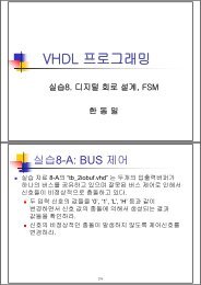
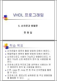
Fig. 2 shows the ratio of measured to incident
wave amplitudes versus relative water depth. The
energy transport approach gives the measured wave
amplitude almost equal to the incident wave amplitude,
while the mass transport approach gives the
measured one different from the incident one by the
ratio of approximately CrC e. This implies that, for
the Boussinesq equations of Nwogu, the internal
generation of waves can be made properly by the
energy transport approach rather than the mass transport
approach. The value of khs5p is far beyond
the traditional deep water limit of khsp , beyond
which the equations of Nwogu yield large errors in
the dispersion. Although there is a point in going to
large value of kh for a wide range demonstration
that Ce
works better than C, the equations are
useless for the value of kh much larger than p.
Fig. 2. Ratio of amplitude of internally generated sinusoidal waves to target one vs. relative water depth; osenergy transport, xsmass
transport, solid linesCrC . e

( )
C. Lee et al.rCoastal Engineering 42 2001 155–162 161
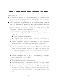
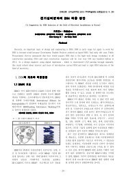
Fig. 3. Normalized surface elevations of internally generated cnoidal waves with different heights using energy transport approach; solid
linesnumerical solution, dashed linesexact solution.
Thirdly, cnoidal waves with different heights are
internally generated in shallow water using the energy
transport approach. The wave period is Ts20 s
and the water depth is hs10 m. The wave heights
are Hs0.1, 0.5, 3 m, so the Ursell numbers are
Ur
s0.05, 0.24, 1.44, respectively. The computa-
tional domain consists of an inner domain of 8 L and
sponge layers at both the right and left boundaries.
The wave generation point is located at the mid-point
of the inner computational domain.
Fig. 3 shows a comparison of the numerical solution
of the surface elevation to the exact solution at
the time ts10T. In the figure, the horizontal distance
is normalized by the wavelength obtained by
the linearized dispersion relation. For the case of
Hs0.1 m, the waves simulated are almost the same
as the sinusoidal waves. Good agreement is observed
between the numerical solution to the exact one
which shows the capability of the present technique
in generating nonlinear waves as well as linear sinusoidal
waves. As the wave height is larger, the wave
crest is steeper, the trough is flatter, the wavelength
is longer, and the phase speed is faster. These are the
characteristics of nonlinear shallow-water waves.
4. Conclusion
It is studied to find out whether the mass transport
or the energy transport is a proper approach for
internally generating waves in the extended Boussinesq
equations of Nwogu Ž 1993 .. The geometric
optics approach is used to get analytically the phase
and energy velocities for the linearized Boussinesq
equations of Nwogu. The variables of the surface
elevation and the particle velocity in the equations of
Nwogu are placed in a staggered grid system. Sponge
layers are placed at the boundaries in order to minimize
wave reflections from the boundaries.
In a horizontally one-dimensional domain, both
the cnoidal and sinusoidal waves are generated inside
the computational domain. It is found that the

162
( )
C. Lee et al.rCoastal Engineering 42 2001 155–162
waves which pass through the wave generation point
cause no serious numerical distortion while the incident
waves are generated at the point. The numerical
results of internal generation of sinusoidal waves,
with different water depths ranging from shallow to
deep waters, show that the energy transport approach
gives wave amplitudes properly. However, the mass
transport approach gives wave amplitudes different
from the desired ones by the ratio of phase to energy
velocities. The technique of internal generation of
waves shows the capability of generating nonlinear
cnoidal waves as well as linear sinusoidal waves.
Although the numerical experiment supports that the
energy transport is a proper approach to internally
generating waves in the extended Boussinesq equations,
a theoretical investigation would be much
valuable.
Acknowledgements
The first author wishes to acknowledge the financial
support of the Korea Science and Engineering
Foundation Ž no. 2000-1-31100-001-3.
during the visit
of the University of Delaware. The second author
wishes to acknowledge the financial support of the
Korea Science and Engineering Foundation Žno.
1999-2-311-005-3 ..
References
Boussinesq, J.V., 1872. Theorie ´ des ondes et des remous qui se
propaent le long d’un canal rectangulaire horizontal, en communiquant
au liquide contenu dans ce canal des vitesses
sensiblement pareilles de la surface au dond. J. Math. Pures
Appliq. 17, 55–108.
Chen, Y., Liu, P.L.-F., 1995. Modified Boussinesq equations and
associated parabolic models for water wave propagation. J.
Fluid Mech. 288, 351–388.
Chen, Q., Madsen, P.A., Schaffer, ¨ H.A., Basco, D.R., 1998.
Wave–current interaction based on an enhanced Boussinesq
approach. Coastal Eng. 33, 11–39.
Copeland, G.J.M., 1985. A practical alternative to the Amild-slopeB
wave equation. Coastal Eng. 9, 125–149.
Larsen, J., Dancy, H., 1983. Open boundaries in short wave
simulations—a new approach. Coastal Eng. 7, 285–297.
Lee, C., Suh, K.D., 1998. Internal generation of waves for timedependent
mild-slope equations. Coastal Eng. 34, 35–57.
Madsen, P.A., Larsen, J., 1987. An efficient finite-difference
approach to the mild-slope equation. Coastal Eng. 11, 329–351.
Madsen, P.A., Schaffer, ¨ H.A., 1998. Higher-order Boussinesq-type
equations for surface gravity waves: derivation and analysis.
Philos. Trans. R. Soc. London A 356, 3123–3184.
Madsen, P.A., Sorensen, O.R., 1992. A new form of the Boussinesq
equations with improved linear dispersion characteristics:
Part 2. A slowly varying bathymetry. Coastal Eng. 18, 183–
204.
Madsen, P.A., Murray, R., Sorensen, O.R., 1991. A new form of
the Boussinesq equations with improved linear dispersion
characteristics. Coastal Eng. 15, 371–388.
Nwogu, O., 1993. Alternative form of Boussinesq equations for
nearshore wave propagation. J. Waterw., Port, Coastal Ocean
Eng. 119, 618–638.
Peregrine, D.H., 1967. Long waves on a beach. J. Fluid Mech. 27,
815–827.
Press, W.H., Teukolsky, S.A., Vetterling, W.T., Flannery, B.P.,
1992. Numerical Recipes in Fortran: The Art of Scientific
Computing. 2nd edn. Cambridge Univ. Press, pp. 42–47.
Radder, A.C., Dingemans, M.W., 1985. Canonical equations for
almost periodic, weakly nonlinear gravity waves. Wave Motion
7, 473–485.
Suh, K.D., Lee, C., Park, W.S., 1997. Time-dependent equations
for wave propagation on rapidly varying topography. Coastal
Eng. 32, 91–117.
Wei, G., Kirby, J.T., Grilli, S.T., Subramanya, R., 1995. A fully
nonlinear Boussinesq model for surface waves: Part 1. Highly
nonlinear unsteady waves. J. Fluid Mech. 294, 71–92.
Wei, G., Kirby, J.T., Sinha, A., 1999. Generation of waves in
Boussinesq models using a source function method. Coastal
Eng. 36, 271–299.
Yoon, S.B., Lee, J.I., Lee, J.K., Chae, J.W., 1996. Boundary
treatment techniques of numerical model for the prediction of
harbor oscillation. J. Korean Soc. Civ. Eng. 16, 53–62, ŽIn
Korean ..