ENT 108-099 - IJME

Section ENT 108-099
Algorithmic Complexity Measure and Lyapanov matrices of the
Dynamical Systems
Davoud Arasteh
Department of Electronic Engineering Technology
Southern University, Baton Rouge, LA 70813
davouda@engr.subr.edu
Abstract
The problem of distinguishing order from disorder in dynamical systems can be answered by
certain quantities such as Lyapanov exponents, fractal dimensions, power spectrum density, and
algorithmic complexity measures. In this paper, we have compared two approaches to evaluate
the order and disorder in dynamic systems behavior. First, this is done by mapping the system
output signal to a binary string and calculating the complexity measure of the time-series data.
The results from algorithmic complexity are compared with the results from Lyapunov metrics
computation. Using these two metrics, we can distinguish noise from chaos and order. This is
important because modern engineering disciplines deal with signals acquired in the form of time
series. The signals obtained from biological, electrical or mechanical systems appear to be
complex. Therefore by extracting their characteristic features in such processes, one can make a
correlation to a certain class of perception or behavior in cognitive sciences. This can be used for
better analysis, control and diagnosis.
Introduction
In this paper we have addressed two practical approaches to evaluate the order and disorder in
nonlinear systems output signal using algorithmic complexity measure [1,2,3] and largest
Lyapanov exponent [4,5]. Mapping the system output signal to a binary string and calculating the
complexity measure of the time-series data, does the characterization of strange attractors by the
pattern formation in phase space attractors. The results obtained from complexity measure are
compared with the results from Lyapunov metrics computation. In nonlinear chaotic systems
small changes in initial conditions lead eventually to large changes in the behavior of the system.
Nevertheless the system remains stable due to its deterministic nature, this occurs because the
chaotic attractors with fractal geometry are confined in a certain region in phase space. For
example in neural systems the divergence from initial state is the fundamental characteristics of
perception to distinguish very close perceptual entities. The artificial cognitive informatics is
concerned with the extraction of characteristic features, their measurement and characterization
of phase space patterns in the processes related to perception and cognition. Signals obtained
from such processes like EEG, ECG or behavioral signals appear to be random. Despite the fact
that, these signals are not random and can be classified as chaotic [6,7,8,9,10]. There are several
metrics to measure chaos, depending on what one wants to characterize in the chaotic trajectory.
Certain quantities such as Lyapanov exponents, fractal dimensions, K-entropy, algorithmic
complexity and power spectrum analysis have been used as screening tools to detect chaos in
nonlinear systems. But methods like Fourier transform, and the resulting power spectrum
Proceedings of The 2006 IJME - INTERTECH Conference

density, fails to distinguish between chaos and noise, because both phenomena are broadband.
This paper deals with the fundamental concept of measuring chaos in dynamical systems through
algorithmic complexity measure and Lyapanov exponents. Algorithmic complexity is a useful
practical tool to characterize spatiotemporal patterns of nonlinear dynamical systems. Both
metrics are capable of distinguishing chaos from order but only complexity metric is capable of
distinguishing deterministic chaos from random noise. In the next section, we introduce the
concept of algorithmic complexity.
Mathematical background
Algorithmic complexity theory defines randomness based only on the characteristics of the
signal, without any knowledge of the source of the data. Application of algorithmic complexity
in multi-dimensional discrete and continuous dynamical systems as a characterizing parameter is
discussed in [11]. We have used Henon discrete map, and forced-dissipative oscillator system to
exemplify and illuminate the concept. We will see that for continuous nonlinear dynamical
system algorithmic complexity measure is as powerful as other characteristics like spectrum of
dimensions and entropies. The numerical effort needed to extract these spectra is rather large.
This limits their determination to systems with dimensionality lower than ten. Therefore it is
necessary to develop analytical tools in order to characterize chaotic motion in high-dimensional
dynamical systems, e.g. spatiotemporal turbulence, or poorly stirred chemical reactions.
The algorithmic complexity of a string is defined to be the length in bits of the shortest algorithm
required for a computer to produce the given string. For our purposes it is not necessary to assign
an absolute value for the complexity of a string of bits. This means relative values are always
sufficient. The shortest algorithms are referred to as minimal programs. The complexity of a
string is thus the length in bits of the minimal program necessary to produce the given string. The
definition of a random number can now be given as any binary string whose algorithmic
complexity is judged to be essentially equal to the length of the string. Qualitatively, the
information embodied in a random number cannot be reduced or compressed to a more compact
form. As the string S grows in length, the length of program grows like n, and the length of the
computer program in bits is essentially the same as the length of S. Such a string satisfies the
definition of a random number since the algorithmic complexity of the string is essentially the
same as the length in bits of the string.
One of the major challenges in chaotic dynamics is to extract a meaningful signal from data that
have every appearance of being random. Clearly algorithmic complexity is a concept aimed
specifically at the problem of distinguishing between the random and the nonrandom.
Nevertheless it can distinguish between chaotic, quasi-periodic, and periodic signals. The
problem lies in determining a computable measure of complexity. No absolute measure is
possible because minimal programs by definition correspond to random numbers, and it is not
possible to determine a truly random number in any formal system. Nevertheless, it is possible to
define a measure of complexity. A relative measure is sufficient for many purposes. For the first
time Kasper and Schuster applied this idea to dynamic systems exhibiting chaos based on work
of Lempel and Ziv. The measure of complexity introduced by Lempel and Ziv is referred as LZ
complexity for brevity. The LZ complexity measures the number of distinct patterns that must be
copied to reproduce a given string. Therefore the only computer operations considered in
constructing a string are copying old patterns and inserting new ones. Briefly described, a string
S is scanned from left to right and complexity counter c (S) increased by one unit every time a
Proceedings of The 2006 IJME - INTERTECH Conference

new sub-string of consecutive digits is encountered in the scanning process. The resultant
number c (S) is the complexity measure of the string S. Clearly any procedure such as this will
over estimate the complexity of strings, but nevertheless we expect comparisons to be
meaningful.
Our efforts here are directed toward outlining a computational algorithm and giving examples of
the LZ complexity measure for various dynamic systems. In quantifying these ideas it becomes
necessary to introduce certain definitions. Let A denote the alphabet of symbols from which the
finite length sequences S are constructed and denote the length of these sequences as L (S) = n.
A sequence S may be written in the form S = S1S2S3...Sn, where Si is mapped from phase space
attractor pattern of a dynamic system based on a mapping rule. The vocabulary of a sequence S,
denoted by V (S), is the set of all substrings of S. The LZ complexity of a given string S is the
number of insertions of new symbols required to reconstruct S, where every attempt is made to
construct S by copying alone without inserting any new symbols. The process is iterative and the
first symbol must always be inserted. Notice that the minimum value for LZ complexity is two.
Furthermore the LZ complexity measure for a given string S is unique and only relative values of
c (n) are meaningful. In particular it is the comparison with the complexity of the random string
that is meaningful. That is one should always compare the LZ complexity of a given string to the
LZ complexity of random strings of the same length, lim n→∞ [c (n)/b (n)], where for a random
string of length n, the LZ complexity is given by b (n) = n/log 2 (n). Fig. 1 shows the complexity
measure calculation flowchart.
Results
The usefulness of the algorithmic complexity measure as a characteristic metrics in dynamic
systems to distinguish the order from disorder is studied next. In this approach, the phase space
pattern of a certain nonlinear system is mapped to an array of symbols. Then the algorithmic
complexity of the resulting bit string is calculated. Our first example is a famous discrete map
called Henon map. The Henon map is a prototypical 2-D invertible iterated dynamical with
chaotic solutions proposed by the French astronomer Michel Henon in 1976 [12]; as a simplified
model of the Poincare map for the Lorenz model. In 1963 the meteorologist Edward Lorenz
observed that a dynamical system with three coupled first-order nonlinear differential equations
could lead to completely chaotic trajectories [13]. Non- linearity is a necessary, but not sufficient
condition of chaos. It is necessary condition, because linear differential equations can be solved
by Fourier transform procedures and do not lead to chaos. The system Lorenz used to model the
dynamics of weather differs from Hamiltonian systems mainly by its dissipativity.
Proceedings of The 2006 IJME - INTERTECH Conference

Start
(String
length N)
C=1
L=1
I=0
K=1
K MAX =1
S(I+K)=S(L+K)
YES
K=K+1
NO
(I+K)>N
NO
S (I+K)=S(L+K)
NO
YES
K MAX =K
C=C+1
YES
I=I+1
END
I=L
YES
K=1
NO
YES
C=C+1
L=L+KMAX
(L+1) > N
NO
Figure 1
Flowchart for calculating LZ complexity for string S with length N
A dissipative system is not conservative but “open”, with an external control parameter that can
be tuned to critical values causing the transitions to chaos. Henon map can illustrate the basic
concepts of complex dynamical systems from non-linearity to chaos with rather simple
computer-assisted methods. Henon map is defined by following quadratic (nonlinear) recursive
map: X n+1
= 1 - a X n
2
+ Yn , Y n +1 = b X n
Where 0

is increased further beyond a critical value a 3 =1.05, the period length doubles. If “a” is increased
further and further; then the period doubles each time with a sequence of critical values a 2 , a 3 .
But beyond a critical value a, the development becomes more and more irregular and chaotic.
For these values, the mapping is contracting the area and has a trapping region, so it exhibits an
attractor. However, for all values |b|

Figure 2
The LZ complexity of strings constructed from the Henon map as a function of
control parameter “a”
Figure 3
Henon bifurcation diagram vs. control parameter “a”.
Figure 4
Largest Lyapunov exponent as a function of control parameter “a”
Proceedings of The 2006 IJME - INTERTECH Conference

Our next example is a continuous dynamical system called Forced-Dissipative-Oscillator. It is
used as a mathematical model for many physical and engineering systems like forced-dissipative
pendulum and Josephson junction under microwave radiation [14, 15, 16], given by following
dynamical equation: D 2 X+ k(DX) + Sin X = g Cos ( d
t), DX = dX/dt
Control parameters are; “k” as system dissipative coefficient, “g” as external driving force
amplitude, and d
external driving force frequency. Roughly speaking, a dissipative system is not
conservative but “open”, with an external control parameter that can be tuned to critical values
causing the transitions to chaos. More precisely, conservative as well as dissipative systems are
characterized by nonlinear differential equations dx/dt = F (x, G) with a nonlinear function F of
the vector x = (x1, ..., xd) depending on an external control parameter G. While for conservative
systems the volume elements in the corresponding phase space change their shape but retain their
volume in the course of time, the volume elements of dissipative systems shrink as time
increases. In dissipative system, or non-Hamiltonian systems, the area-preserving principle does
not apply. In fact, the sum of all the Lyapunov exponents must be negative for physical
dissipative dynamical system. A one-dimensional map like logistic map there is only one
Lyapunov exponent. If it is negative, the map has either limit point stability or limit cycle
stability. In n-dimensional systems, the stretching and contraction along the principal axis in the
phase space produce a spectrum of Lyapunov exponents. For example in three-dimension the
Lyapunov spectrum is (λ1, λ2, λ3). Stable periodic attractors have only zero and negative
Lyapunov exponents. For example, (λ1= 0, λ2= negative number, λ3 = negative number) where
the zero corresponds to the limit-cycle trajectory itself or (λ1= 0, λ2 = 0, λ3 = negative number)
for an attracting 2-torus. Chaotic attractors have just one finite positive Lyapunov exponent. In
three-dimension systems the spectrum of the Lyapunov exponents is (+, 0, -), where the zero
corresponds to the chaotic trajectory itself, with some trajectories expanding, while others are
contracting. For forced oscillator system we have used both tools to explore the regions of
periodic and chaotic behaviors.
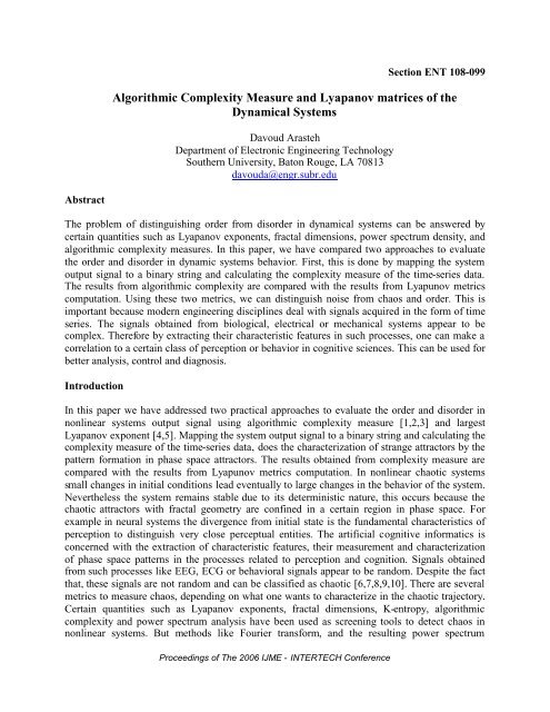
The complexity of the oscillator map is calculated by setting control parameters to following
values. d
= 2/3, k = 0.5, and g is varied in the range [0.9, 1.5], with ∆g = 0.001. An array from
n= 20000 iterations is constructed after removing the transient values for a specific external force
amplitude (g). A digit “1” is mapped into the array if the velocity (DX) of the oscillator is larger
than zero (a pendulum passing its equilibrium state), otherwise digit “0” is inserted in the array.
The choice of using this encoding scheme is based on the symmetrical velocity distribution
function. This function is calculated from distribution density of 80000 phase space points of a
chaotic attractor (Fig. 5), with normalized frequency of 2/3, dissipation coefficient of 0.5, and
external driving amplitude of 1.2. We have computed the algorithmic complexity measure of
each experiment versus the corresponding driving force amplitudes (Fig. 6). For comparison we
have also plotted the bifurcation diagram (Fig. 7) as well as the largest Lyapunov exponent (Fig.
8). The results indicate distinct regions corresponding to chaotic and periodic behaviors. When
Forced-Dissipative-Oscillator system has periodic behaviors of 1-cycle, 2-cycle, … and
displayed in bifurcation windows, the LZ complexity measure is small. This corresponds to the
limit-cycle trajectory or an attracting 2-torus. On the other hand chaotic attractors with some
trajectories expanding, while others are contracting, have large LZ complexity, this is nicely
mirrored by the increasing values of c (n) plot. For this system there is only one finite positive
Lyapanov exponent and only one symbolic Lyapanov spectrum of the form (+, 0, -), where the
zero corresponds to the chaotic trajectory itself, with some trajectories expanding, while others
Proceedings of The 2006 IJME - INTERTECH Conference

are contracting.
Figure 5
Forced-dissipative oscillator strange attractor and its Poincare map
g=1.2, k=0.5, ω d =2/3
Figure 6
Forced-Dissipative-Oscillator algorithmic complexity measure versus control
parameter g, amplitude of the external force (0.9

Figure 7
FDO bifurcation diagram versus control parameter g, amplitude of the external
force (0.9

experiment. We observed that the algorithmic complexity of the chaotic responses is much
higher than periodic responses. In this work we showed the usefulness of LZ complexity
measure as a metric to characterize the patterns of discrete and continuous dynamical systems
with chaotic and periodic responses. This is important because it provides a computational metric
to find and classify the complex patterns.
References
[1] A. Lempel, J. Ziv, “On the complexity of individual sequences”, IEEE Transaction in
Information Theory Vol. IT-22, p. 75, 1976.
[2] A. Lempel, J. Ziv, “Compression of Individual Sequences via Variable-Rate Coding”, IEEE
Transaction in Information Theory, Vol. IT-24, NO. 5, 1978.
[3] Torres ME and L. G. Gamero, “Relative Complexity Changes in Time Series using
Information Measures”, Physica A, Vol. 286, Iss. 3-4, pp.457-473, Oct. 2000.
[4] A. Wolf, J. B. Swift, H. L. Swinney, and J. A. Vastano, “Determining Lyapunov exponents
from a time series”, Physica D, vol. 16, pp. 285–317, 1985.
[5] W. Kinsner, “Characterizing Chaos Through Lyapunov Metrics”, IEEE Transactions on
Systems, Man, and Cybernetics, Part C, Vol. 36, No. 2, 2006.
[6] Szczepanski J, JM Amigo, E Wajnryb and MV Sanchez-Vives, “Application of Lempel–Ziv
complexity to the analysis of neural discharges”, Network: Computation in Neural Systems, 14
pp. 335–350, 2003.
[7] Gonzalez Andino SL, Grave de Peralta Menendez R, Thut G, Spinelli L, Blanke O, Michel
CM, Seeck M, Landis T., “Measuring the complexity of time series: an application to
neurophysiological signals”. Hum Brain Mapp. 2000 Sep;11(1):46-57.
[8] Watanabe TA, Cellucci CJ, Kohegyi E, Bashore TR, Josiassen RC, Greenbaun NN, Rapp PE.
“The algorithmic complexity of multichannel EEGs is sensitive to changes in behavior”
Psychophysiology, Jan;40(1):77-97, 2003
[9] Jaeseung, J., Jeong-Ho C., Kim, S. Y. & Seol-Heui, H., “Nonlinear dynamical analysis of the
EEG in patients with Alzheimer’s disease and vacular dementia”, Clin., Neurophysiol 18(1):58-
67, 2001.
[10] Huang L, Fengchi Ju, Enke Zhang, Jingzhi Cheng, “Real-time Estimation of Depth of
Anaesthesia Using the Mutual Information of Electroencephalograms”, Proceedings of the 1st
International IEEE EMBS Conference on Neural Engineering Capri Island. Italy March 20-22,
2003.
[11] F. Kasper, H.G. Shuster, “Easily calculable measure for the complexity of spatiotemporal
patterns.” Physical Review A, Vol. 36, p. 832, 1987.
[12] M. Henon, “A two-dimensional mapping with a strange attractor”, Comm. Math. Phys. Vol.
50, p. 69, 1976.
Proceedings of The 2006 IJME - INTERTECH Conference

[13] E. N. Lorentz, ”Deterministic Nonperiodic Flow”, J. Atoms Sci., Vol. 20, p.130, 1963. In
“Universality in Chaos”, edited by P. Civitanovic, Adam Hilger, 1989.
[14] C. B. Whan and C. J. Lobb, “Complex Dynamical Behavior in RLC-shunted Josephson
Junctions”, IEEE Transaction on Superconductivity, Vol. 5, No. 2, June 1995.
[15] D. D’ Humierres, M. R. Beasley, B. A. Libchaber, “Chaotic states and routes to chaos in the
forced pendulum”, Physical Review A, Vol. 26, No. 6, p. 3483, 1982.
[16] B.A. Huberman, J. P. Crutchfield, N. H. Packard, “Noise phenomena in Josephson
Junction”, Applied Physics Letter, Vol. 37, 750, 1980.
Biography
Davoud Arasteh serves as an assistant professor of Electronic Engineering Technology at
Southern University of Baton Rouge. His research interests include Mobile Computing, Network
Security, Nonlinear Dynamical Systems, Computer Vision, and Technology Based Engineering
Education. He is the chair of departmental curriculum committee and is a member of ASEE,
IEEE, IEEE Computer Society, IEEE Electromagnetic Compatibility Society, and IEEE
Computational Intelligence Society.
Proceedings of The 2006 IJME - INTERTECH Conference