Electric Vehicle Energy Usage Modeling and Measurement ... - IJME
Electric Vehicle Energy Usage Modeling and Measurement ... - IJME
Electric Vehicle Energy Usage Modeling and Measurement ... - IJME

Create successful ePaper yourself
Turn your PDF publications into a flip-book with our unique Google optimized e-Paper software.
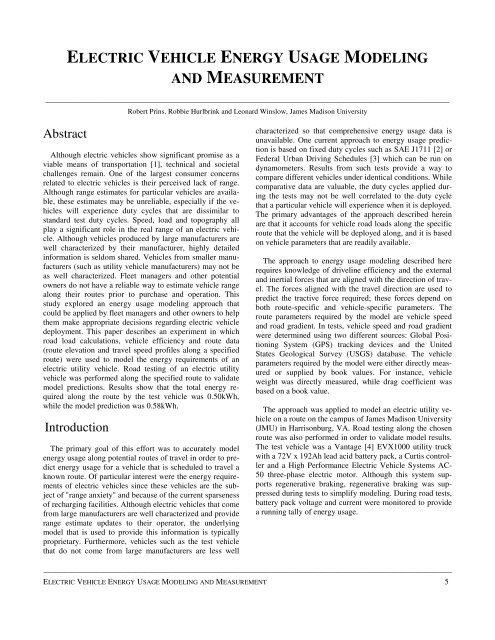
ELECTRIC VEHICLE ENERGY USAGE MODELING<br />
AND MEASUREMENT<br />
——————————————————————————————————————————————–———–<br />
Robert Prins, Robbie Hurlbrink <strong>and</strong> Leonard Winslow, James Madison University<br />
Abstract<br />
Although electric vehicles show significant promise as a<br />
viable means of transportation [1], technical <strong>and</strong> societal<br />
challenges remain. One of the largest consumer concerns<br />
related to electric vehicles is their perceived lack of range.<br />
Although range estimates for particular vehicles are available,<br />
these estimates may be unreliable, especially if the vehicles<br />
will experience duty cycles that are dissimilar to<br />
st<strong>and</strong>ard test duty cycles. Speed, load <strong>and</strong> topography all<br />
play a significant role in the real range of an electric vehicle.<br />
Although vehicles produced by large manufacturers are<br />
well characterized by their manufacturer, highly detailed<br />
information is seldom shared. <strong>Vehicle</strong>s from smaller manufacturers<br />
(such as utility vehicle manufacturers) may not be<br />
as well characterized. Fleet managers <strong>and</strong> other potential<br />
owners do not have a reliable way to estimate vehicle range<br />
along their routes prior to purchase <strong>and</strong> operation. This<br />
study explored an energy usage modeling approach that<br />
could be applied by fleet managers <strong>and</strong> other owners to help<br />
them make appropriate decisions regarding electric vehicle<br />
deployment. This paper describes an experiment in which<br />
road load calculations, vehicle efficiency <strong>and</strong> route data<br />
(route elevation <strong>and</strong> travel speed profiles along a specified<br />
route) were used to model the energy requirements of an<br />
electric utility vehicle. Road testing of an electric utility<br />
vehicle was performed along the specified route to validate<br />
model predictions. Results show that the total energy required<br />
along the route by the test vehicle was 0.50kWh,<br />
while the model prediction was 0.58kWh.<br />
Introduction<br />
The primary goal of this effort was to accurately model<br />
energy usage along potential routes of travel in order to predict<br />
energy usage for a vehicle that is scheduled to travel a<br />
known route. Of particular interest were the energy requirements<br />
of electric vehicles since these vehicles are the subject<br />
of "range anxiety" <strong>and</strong> because of the current sparseness<br />
of recharging facilities. Although electric vehicles that come<br />
from large manufacturers are well characterized <strong>and</strong> provide<br />
range estimate updates to their operator, the underlying<br />
model that is used to provide this information is typically<br />
proprietary. Furthermore, vehicles such as the test vehicle<br />
that do not come from large manufacturers are less well<br />
characterized so that comprehensive energy usage data is<br />
unavailable. One current approach to energy usage prediction<br />
is based on fixed duty cycles such as SAE J1711 [2] or<br />
Federal Urban Driving Schedules [3] which can be run on<br />
dynamometers. Results from such tests provide a way to<br />
compare different vehicles under identical conditions. While<br />
comparative data are valuable, the duty cycles applied during<br />
the tests may not be well correlated to the duty cycle<br />
that a particular vehicle will experience when it is deployed.<br />
The primary advantages of the approach described herein<br />
are that it accounts for vehicle road loads along the specific<br />
route that the vehicle will be deployed along, <strong>and</strong> it is based<br />
on vehicle parameters that are readily available.<br />
The approach to energy usage modeling described here<br />
requires knowledge of driveline efficiency <strong>and</strong> the external<br />
<strong>and</strong> inertial forces that are aligned with the direction of travel.<br />
The forces aligned with the travel direction are used to<br />
predict the tractive force required; these forces depend on<br />
both route-specific <strong>and</strong> vehicle-specific parameters. The<br />
route parameters required by the model are vehicle speed<br />
<strong>and</strong> road gradient. In tests, vehicle speed <strong>and</strong> road gradient<br />
were determined using two different sources: Global Positioning<br />
System (GPS) tracking devices <strong>and</strong> the United<br />
States Geological Survey (USGS) database. The vehicle<br />
parameters required by the model were either directly measured<br />
or supplied by book values. For instance, vehicle<br />
weight was directly measured, while drag coefficient was<br />
based on a book value.<br />
The approach was applied to model an electric utility vehicle<br />
on a route on the campus of James Madison University<br />
(JMU) in Harrisonburg, VA. Road testing along the chosen<br />
route was also performed in order to validate model results.<br />
The test vehicle was a Vantage [4] EVX1000 utility truck<br />
with a 72V x 192Ah lead acid battery pack, a Curtis controller<br />
<strong>and</strong> a High Performance <strong>Electric</strong> <strong>Vehicle</strong> Systems AC-<br />
50 three-phase electric motor. Although this system supports<br />
regenerative braking, regenerative braking was suppressed<br />
during tests to simplify modeling. During road tests,<br />
battery pack voltage <strong>and</strong> current were monitored to provide<br />
a running tally of energy usage.<br />
——————————————————————————————————————————————————–<br />
ELECTRIC VEHICLE ENERGY USAGE MODELING AND MEASUREMENT 5
——————————————————————————————————————————————–————<br />
Methodology<br />
Prediction of energy usage requires a model of the vehicle<br />
<strong>and</strong> the route that the vehicle will travel. After the model<br />
was developed <strong>and</strong> a prediction obtained, the predicted energy<br />
usage was compared to the measured energy usage<br />
along the route. A measure of energy usage along the route<br />
was obtained by monitoring battery energy output while<br />
driving the route. This section describes the vehicle model,<br />
route model, energy usage prediction <strong>and</strong> energy usage<br />
measurement.<br />
<strong>Vehicle</strong> Model<br />
The vehicle model used in this study was based on the<br />
external <strong>and</strong> inertial forces acting on the vehicle that are<br />
aligned with the direction of travel as described by Gillespie<br />
[5]. These external forces are in equilibrium with the tractive<br />
force applied by the wheels:<br />
F T = F R + F D + F G + F A (1)<br />
where,<br />
F T = tractive force<br />
F R = rolling resistance force<br />
F D = force due to drag<br />
F G = force due to gravity<br />
F A = force due to acceleration in the direction of travel<br />
Rolling resistance addresses forces related to contact between<br />
tire <strong>and</strong> road surfaces, drag is due to wind resistance,<br />
the force of gravity accounts for the force required to<br />
change elevation, the acceleration force accounts for the<br />
force required to change speed. Equation 1 can be exp<strong>and</strong>ed<br />
to show the terms associated with each force:<br />
where,<br />
W =<br />
f r =<br />
ρ =<br />
c d =<br />
A =<br />
v =<br />
θ =<br />
g =<br />
a =<br />
F T = W f r + (1/2) ρ c d A v 2 + W sinθ + (W/g) a (2)<br />
weight of loaded vehicle<br />
rolling resistance coefficient<br />
air density<br />
drag coefficient<br />
frontal area<br />
air speed<br />
angle of road<br />
acceleration due to gravity<br />
acceleration in direction of travel<br />
Determination of Rolling Resistance Force<br />
The force of rolling resistance is due to the deformation<br />
of tires rolling along the road surface. Rolling resistance is<br />
affected by factors such as tire pressure, pavement characteristics<br />
<strong>and</strong> tread conditions. During road testing, tire pressure<br />
was maintained at a consistent level while variation in<br />
road surface <strong>and</strong> tread conditions were noted to be negligible.<br />
The weight of the loaded vehicle was measured using a<br />
drive-on scale at a local lumber company; the measured<br />
weight was 14,055N (3,160lb). The rolling resistance coefficient<br />
was determined from coast-down tests. In a coastdown<br />
test, the vehicle is driven at a constant speed <strong>and</strong> then<br />
allowed to “coast down” to a stop [6]. <strong>Vehicle</strong> speed is recorded<br />
at known time intervals during the coast-down period<br />
so that deceleration can be calculated. If the road is flat <strong>and</strong><br />
the speed is relatively low, gravitational force <strong>and</strong> drag<br />
force <strong>and</strong> can be neglected <strong>and</strong> all of the deceleration can be<br />
attributed to rolling resistance. As a perfectly flat test surface<br />
was not available for this effort, coast-down tests were<br />
performed in two directions on a reasonably flat test surface<br />
in order to determine the rolling resistance coefficient. The<br />
results from each direction were used to provide a two-way<br />
average of deceleration. Using this approach, the rolling<br />
resistance coefficient was determined to be 0.014, which<br />
lies within typical values reported by Gillespie [5].<br />
Determination of Drag Force<br />
The force due to drag accounts for wind resistance <strong>and</strong> is<br />
dependent upon the density of air, the shape of the vehicle,<br />
the frontal area of the vehicle <strong>and</strong> the air speed of the vehicle.<br />
Air density was determined based on temperature, pressure<br />
<strong>and</strong> humidity conditions as provided by a h<strong>and</strong>held<br />
weather station at the time of testing. Drag coefficients can<br />
be directly measured in wind tunnels or determined from<br />
high-speed coast-down tests. The vehicle speed was limited<br />
to ~11.5m/s (25MPH), which was determined to be too slow<br />
to get reliable coast-down data for drag force. A book value<br />
of 0.45 associated with similarly shaped pickup trucks [5]<br />
was used for modeling purposes. The frontal area was determined<br />
by direct measurement of the vehicle to be 2.16m 2 .<br />
Testing was done in calm conditions so that air speed could<br />
be well approximated by ground speed. Ground speed along<br />
the route was determined by a GPS tracker <strong>and</strong> verified by<br />
comparison to wheel speed, as shown in Figure 1.<br />
The wheel speed shown in Figure 1 was determined by<br />
monitoring the motor speed signal from the controller while<br />
traveling the route. A combination of the motor speed with<br />
known driveline ratios <strong>and</strong> tire size results in wheel speed.<br />
Figure 1 shows that the GPS-tracker-based speed <strong>and</strong> the<br />
wheel speed compare well along the route.<br />
——————————————————————————————————————————————–————<br />
6 INTERNATIONAL JOURNAL OF MODERN ENGINEERING | VOLUME 13, NUMBER 1, FALL/WINTER 2012
——————————————————————————————————————————————–————<br />
Label Variable Value Unit Source<br />
W weight of loaded vehicle 14055<br />
(3160)<br />
Table 1. Road-Load Variables, Values <strong>and</strong> Sources<br />
N<br />
(lb)<br />
drive-on scale<br />
f r rolling resistance coefficient 0.014 N/A coast down test<br />
r air density varies kg/m 3 equation based on parameters measured at<br />
time of test<br />
c d drag coefficient 0.45 N/A book value for similar vehicle<br />
A frontal area 2.16 m 2 measurement of vehicle<br />
v air <strong>and</strong> ground speed varies continuously m/s route model<br />
q angle of road varies continuously degrees route model<br />
g acceleration due to gravity 9.81 m/s 2 book value<br />
a acceleration varies continuously m/s 2 route model<br />
Table 1 shows that a book value was relied upon for one<br />
variable (drag coefficient) while values for the other variables<br />
were measured. Some of the variables remained constant<br />
during testing while vehicle speed, road angle <strong>and</strong> acceleration<br />
varied continuously. The continuous variables<br />
were measured at a frequency of 1Hz which is the collection<br />
rate of the GPS trackers used in this study.<br />
Route Model<br />
Figure 1. Comparison of GPS-Speed <strong>Measurement</strong> to Wheel-<br />
Speed <strong>Measurement</strong><br />
Determination of Gravitational Force<br />
The force due to gravity accounts for changes in elevation<br />
<strong>and</strong> is dependent upon vehicle weight <strong>and</strong> change in elevation.<br />
The weight of the loaded vehicle was measured as described<br />
above; the road angle was based on sequential GPS<br />
measurements of position <strong>and</strong> elevation.<br />
Determination of Force Due to<br />
Acceleration in the Direction of Travel<br />
The force due to acceleration in the direction of travel<br />
accounts for changes in vehicle speed <strong>and</strong> is dependent on<br />
vehicle mass <strong>and</strong> change in travel speed. The weight of the<br />
loaded vehicle was measured as described above; changes<br />
in travel speed were based on sequential GPS-tracker-based<br />
speed measurements. Table 1 indicates the values of the<br />
variables in Equation (2).<br />
The route model consists of the elevation profile of the<br />
path of travel as well as an expected speed profile of the<br />
vehicle along the path. The elevation profile of the JMU<br />
route used in the energy calculations came from two<br />
sources: GPS trackers <strong>and</strong> the USGS database. The source<br />
of the speed profile was again the GPS trackers.<br />
Determination of Elevation Profile<br />
For this study, GPS trackers <strong>and</strong> USGS data were the<br />
sources of elevation data. In order to determine the elevation<br />
profile of the path, four different methods were used<br />
which were then compared. The four methods were:<br />
• Raw elevation data from Trimble Geo XH GPS<br />
tracker<br />
• Raw elevation data from Garmin eTrex Vista<br />
GPS tracker<br />
• Post-processed (differentially corrected) elevation<br />
data from the Trimble Geo XH GPS tracker<br />
• Elevation data from USGS database<br />
——————————————————————————————————————————————————–<br />
ELECTRIC VEHICLE ENERGY USAGE MODELING AND MEASUREMENT 7
——————————————————————————————————————————————–————<br />
The GPS-tracker-based elevation data were collected by<br />
traveling the route with two active GPS trackers, which<br />
provided elevation data at 1Hz intervals. The GPS trackers<br />
used to conduct this study were a Trimble Geo XH <strong>and</strong> a<br />
Garmin eTrex Vista. The Trimble Geo XH is survey grade,<br />
while the Garmin eTrex Vista is recreational grade. The<br />
Garmin eTrex Vista produces lower accuracy position data<br />
but has a built-in barometric pressure sensor which allows<br />
relative elevation readings to be taken without relying on<br />
satellites.<br />
The Trimble GPS data were also post-processed using<br />
differential correction to provide a third set of elevation<br />
data. Differential correction methods remove anomalies due<br />
to issues in the interaction between satellites <strong>and</strong> GPS receivers<br />
(typically due to atmospheric conditions) based on<br />
readings from nearby GPS receivers that are in a fixed location<br />
[7]. Because the Trimble tracker is survey grade, differentially<br />
corrected route data from the Trimble tracker is<br />
considered to be the most reliable source of route model<br />
data used in this study.<br />
The fourth set of elevation data was sourced from a<br />
USGS database. The USGS has image-based digital elevation<br />
models (DEMs) published online that have a resolution<br />
of 10 meters. This means that in an image, every 10-meter<br />
by 10-meter pixel is assigned an elevation value [8]. For the<br />
case described here, the route was entered into ArcMap<br />
(geospatial analysis software) <strong>and</strong> the elevation data for<br />
points along the route were extracted from the appropriate<br />
DEM.<br />
Elevation data from each of the four methods were processed<br />
to provide elevation relative to a start point. Figure 2<br />
shows the relative elevation profiles resulting from the application<br />
of the four methods discussed above.<br />
beginning of the run, but then follow a similar shape to the<br />
others. One potential problem with relying on USGS data is<br />
observed as a dip near the 7:00 minute mark. The USGS<br />
DEM has 10-meter resolution which is not small enough to<br />
resolve a bridge that was part of the route. In this case, the<br />
USGS DEM provided elevation data for the ravine that the<br />
bridge crosses.<br />
Determination of Speed Profile<br />
The speed profile of the route was determined by traveling<br />
the route at typical speeds with an active GPS tracker.<br />
The GPS trackers provided position data at 1Hz intervals,<br />
vehicle speed was calculated from the difference in position<br />
between sequential position points. The speed profile for the<br />
route is shown in Figure 1. The speed profile used in this<br />
study is based on differentially corrected route data from the<br />
Trimble tracker.<br />
<strong>Energy</strong> <strong>Usage</strong> Prediction<br />
The goal of this effort was to predict the amount of energy<br />
that must be supplied by the battery pack. The amount of<br />
energy required from the battery pack is a function of the<br />
amount of energy required at the wheel <strong>and</strong> vehicle<br />
drivetrain efficiency. <strong>Energy</strong> requirements at the wheel are<br />
based on tractive force predictions while drivetrain efficiency<br />
is based on RPM-specific values published by the motor<br />
manufacturer.<br />
Predictions of energy usage at the wheel are based on the<br />
tractive force model as calculated in Equation (2). Since<br />
some of the tractive force parameters (speed, road angle <strong>and</strong><br />
acceleration) change with each successive time interval, the<br />
energy calculation addresses a single interval. In order to<br />
use tractive force to determine energy usage for a given<br />
interval, the distance across which the tractive force is applied<br />
during the interval must be known, as shown in Equation<br />
(3):<br />
(3)<br />
Figure 2. Elevation Profiles from Four Methods<br />
Figure 2 shows that the Trimble raw, Trimble corrected<br />
<strong>and</strong> USGS elevation data are similar in value <strong>and</strong> shape.<br />
The Garmin elevation data display a ~25m jump near the<br />
where,<br />
∆E wheel,i = energy usage at the wheel to travel<br />
the interval distance ∆d i<br />
F T,i = tractive force during interval i<br />
∆d i = distance traveled during interval i<br />
Equation (3) can be rewritten in terms of speed, as shown<br />
in Equation (4):<br />
——————————————————————————————————————————————–————<br />
8 INTERNATIONAL JOURNAL OF MODERN ENGINEERING | VOLUME 13, NUMBER 1, FALL/WINTER 2012<br />
(4)
——————————————————————————————————————————————–————<br />
where,<br />
∆E wheel,i = energy usage at the wheel to travel for the<br />
interval time ∆t i<br />
F T,i = tractive force during interval i<br />
v i = average speed along path during time<br />
interval i<br />
∆t i = length of time interval i<br />
Equation (5) is an expansion of Equation (4) <strong>and</strong> shows<br />
the tractive force terms from Equation (2). In Equation (5),<br />
terms that are updated for each time interval are given the<br />
interval subscript i.<br />
∆E wheel i = [W f r + (1/2) ρ c d Α v i 2 + W sin(θ i ) +<br />
(W/g)(v i -v i-1 )/∆t i ] v i ∆t i (5)<br />
The amount of energy required from the battery pack depends<br />
on the energy required at the wheel as well as vehicle<br />
drivetrain efficiency. In order to determine the energy required<br />
from the battery pack, an efficiency factor based on<br />
published data from the motor manufacturer that correlates<br />
efficiency to motor RPM at peak load was applied. Motor<br />
RPM was determined from vehicle speed <strong>and</strong> known drive<br />
ratios; motor RPM is continuously variable so that<br />
drivetrain efficiency must be updated for each time interval,<br />
as shown in Equation (6):<br />
∆E battery i × η i = ∆E wheel i (6)<br />
where,<br />
∆E battery i = energy provided from battery pack during<br />
interval i<br />
η = drive efficiency during interval i<br />
∆E wheel i = energy required at wheel during interval i<br />
This method results in a prediction of the incremental<br />
energy provided by the battery pack for each time interval;<br />
the total energy provided by the battery pack along a particular<br />
route is predicted by the summation of the ∆E battery i<br />
values from all of the intervals.<br />
Road Tests<br />
In order to validate the energy usage predictions of the<br />
model, vehicle energy usage was monitored (measured at<br />
the battery pack) while traveling along the route. This was<br />
done by logging battery pack voltage <strong>and</strong> current at 1Hz<br />
time intervals along the route. The amount of energy removed<br />
from the battery during each time interval is the<br />
product of the battery pack voltage, current <strong>and</strong> time interval,<br />
as shown in Equation 7.<br />
E measured,i = V measured,i I measured,i ∆t i (7)<br />
where,<br />
E measured,i = energy removed from battery pack<br />
during interval i<br />
V measured,i = battery pack voltage during interval i<br />
I measured,i = battery pack current during interval i<br />
∆t i = length of time of interval i<br />
This approach results in a measurement of the incremental<br />
energy provided by the battery pack for each time interval;<br />
the total energy provided by the battery pack along a<br />
particular route is the summation of the ∆E measured i values<br />
from all of the intervals.<br />
Results<br />
The results of this effort include the raw speed <strong>and</strong> elevation<br />
data used to construct the route model, battery energy<br />
usage predictions based on tractive force prediction, <strong>and</strong><br />
measured energy usage from road testing.<br />
Figure 3 shows a typical set of elevation <strong>and</strong> speed profile<br />
data for a particular route along with the corresponding energy<br />
usage prediction (based on differentially corrected<br />
Trimble tracker elevation data). <strong>Energy</strong> usage is graphed as<br />
cumulative energy usage so that the final point on the graph<br />
represents the total energy prediction for the route. The dependency<br />
of energy usage predictions on route elevation<br />
<strong>and</strong> speed profiles can be seen in Figure 3. For instance,<br />
note that near the 2:50 minute mark, the vehicle speed is<br />
near zero <strong>and</strong> there is little elevation change which suggests<br />
that little energy input is required. The cumulative energy<br />
graph is nearly flat at this point, which indicates little predicted<br />
energy usage at that time. On the other h<strong>and</strong>, note<br />
that near the 7:00 minute mark, the road increases in elevation<br />
while speed is maintained at a constant ~9m/s<br />
(20MPH), which suggests that significant energy input is<br />
required. The cumulative energy graph has a steep slope at<br />
this time which indicates high predicted energy usage.<br />
Recall that four different methods were used to determine<br />
elevation in the route model. Each method results in a different<br />
route elevation profile, as shown in Figure 2. The<br />
elevation profile variation affects energy usage predictions,<br />
as shown in Figure 4.<br />
The energy values in Figure 4 are graphed as cumulative<br />
energy usage so that the final points on the graph represent<br />
the total energy predictions for the route. Figure 4 also includes<br />
the measured energy from road testing for comparison.<br />
It can be seen that the lines representing the four energy<br />
usage predictions are similar in shape <strong>and</strong> value to the<br />
line that represents measured energy usage. The prediction<br />
——————————————————————————————————————————————————–<br />
ELECTRIC VEHICLE ENERGY USAGE MODELING AND MEASUREMENT 9
——————————————————————————————————————————————–————<br />
with the worst agreement is the one that relies on the Garmin<br />
GPS tracker for elevation profile. All predictions overpredicted<br />
the energy usage required for the entire route,<br />
although not at all points along the route. Table 2 summarizes<br />
the predictions of energy usage along the route from the<br />
four methods, as well as their variation from the measured<br />
energy usage.<br />
Table 2. Total <strong>Energy</strong> to Travel Route<br />
Data Source<br />
Trimble<br />
(corrected)<br />
Total <strong>Energy</strong> to<br />
Travel Route (kWh)<br />
% Variation from<br />
Road Test<br />
0.577 + 14.8<br />
Garmin 0.611 + 21.4<br />
USGS 0.560 + 11.3<br />
Trimble (raw) 0.542 + 7.9<br />
Road Test 0.503 -<br />
(a) Elevation <strong>and</strong> Speed Profiles of Route<br />
Table 2 shows that variation between energy usage measured<br />
during the road test <strong>and</strong> energy usage predictions varies<br />
from 8% to 22%. The major contributor to variation is<br />
the source of the elevation model used to predict energy<br />
usage. The Garmin tracker, which reported an elevation<br />
profile dissimilar to the Trimble tracker <strong>and</strong> the USGS model,<br />
is the source of the elevation model that varies by nearly<br />
22% from the road test values. Although the raw Trimble<br />
tracker data show the lowest variation (8%) relative to road<br />
test data, the differentially corrected output from the Trimble<br />
tracker (Trimble corrected) is likely a better source of<br />
elevation data.<br />
Figure 4 demonstrates that the model over predicts the<br />
measured energy usage. At the end of the route, the total<br />
energy usage predicted by the most reliable model (Trimble<br />
corrected) was 0.58kWh in comparison to a measurement of<br />
0.50kWh; this represents a variation of ~15%.<br />
(b) Prediction of <strong>Energy</strong> <strong>Usage</strong> along Route<br />
Figure 3. <strong>Energy</strong> <strong>Usage</strong> Prediction along Route <strong>and</strong> the Underlying<br />
Elevation <strong>and</strong> Speed Profiles<br />
Figure 4. <strong>Energy</strong> <strong>Usage</strong> Prediction <strong>and</strong> Road Test Results<br />
Discussion<br />
The selected route included ~20m total descent <strong>and</strong> ~55m<br />
total ascent, which is representative of typical routes traveled<br />
on the campus of JMU. It can be seen from Figure 4<br />
that energy usage predictions <strong>and</strong> measured energy usage<br />
exhibit similar form although differences do exist. If the<br />
variation between predicted <strong>and</strong> measured energy usage is<br />
characterized as ~14% (the average variation), different<br />
conclusions could reasonably be drawn. For some purposes,<br />
14% variation may be considered acceptable in which case<br />
an avenue for future work would be to further test <strong>and</strong> validate<br />
the current approach on other routes <strong>and</strong> with other<br />
vehicles to gain confidence that the approach is universally<br />
reliable. For other purposes, 14% variation may be considered<br />
unacceptable in which case further refinement of the<br />
model would be in order.<br />
Efforts directed at model refinement could begin with a<br />
comparison of Figures 4 <strong>and</strong> 3a which suggest that while in<br />
——————————————————————————————————————————————–————<br />
10 INTERNATIONAL JOURNAL OF MODERN ENGINEERING | VOLUME 13, NUMBER 1, FALL/WINTER 2012
——————————————————————————————————————————————–————<br />
general the energy usage models tend to over predict energy<br />
usage, this is especially noticeable from 3:45 - 4:40 minutes<br />
(minimal elevation change combined with varied speeds)<br />
<strong>and</strong> from 6:20 - 7:47 minutes (extended deceleration while<br />
making an ascent). While such observations provide some<br />
insight, it would be ill-advised to make adjustments to the<br />
model in order to better match the measured energy usage<br />
without underst<strong>and</strong>ing the interactions between vehicle<br />
model parameters <strong>and</strong> route model parameters. This suggests<br />
that an avenue for further work would be to continue<br />
to work with the test vehicle under controlled conditions of<br />
slope, speed <strong>and</strong> payload in order to scrutinize the model.<br />
The main strength of using a GPS-tracker approach to<br />
developing a route model is that elevation measurements<br />
along the route are made directly. This means that the model<br />
does not depend on DEMs from the USGS which may not<br />
resolve critical route features. The main weakness of using<br />
the GPS-tracker approach is that the route must be driven<br />
while collecting tracker data. For relatively long routes, the<br />
effect of route features that are not properly resolved by<br />
DEMs may not be significant, in which case predictions of<br />
total energy usage should be reasonably close to actual energy<br />
requirements. This suggests that another avenue for further<br />
work would be development <strong>and</strong> validation of USGSbased<br />
route models with the intent of developing a reliable<br />
prediction of energy usage that does not require physical<br />
presence along the route.<br />
Conclusions<br />
An energy usage model that accounts for the route of an<br />
electric vehicle was applied to a small, electric-powered<br />
utility vehicle traveling a route with significant elevation<br />
variation. A model of tractive force as well as elevation <strong>and</strong><br />
speed profiles of the route provided energy usage predictions<br />
along the route. The predictions were validated by a<br />
road test in which the route was traveled while energy usage<br />
from the battery pack was monitored. At the end of the<br />
route, the total predicted energy usage varied from the<br />
measured energy usage by ~15%.<br />
Paths for future work include continued testing of the<br />
current model along other routes <strong>and</strong> with other vehicles,<br />
refinement of the model, <strong>and</strong> further development of USGSbased<br />
route models.<br />
Acknowledgements<br />
The authors thank Kelly Sites of James Madison University<br />
Facilities Management - Transportation for use of the<br />
electric vehicle <strong>and</strong> the Alternative Fuels <strong>Vehicle</strong> Laborato-<br />
ry (AFV) for providing work space; Dr. Carole Nash, Assistant<br />
Professor in the Department of Integrated Science <strong>and</strong><br />
Technology at James Madison University, for sharing her<br />
expertise in geospatial sensing <strong>and</strong> modeling; <strong>and</strong> Ed Thurnau,<br />
electrical engineer with GE Intelligent Platforms, for<br />
sharing his expertise in signal conditioning <strong>and</strong> processing.<br />
This research was supported in part by the ‘Shen<strong>and</strong>oah<br />
Valley as a National Demonstration Project Achieving 25<br />
Percent Renewable <strong>Energy</strong> by the Year 2025’ under U.S.<br />
Department of <strong>Energy</strong> Grant #DE-EE0003100. The views<br />
expressed are those of the authors <strong>and</strong> do not necessarily<br />
reflect those of the sponsors.<br />
References<br />
[1] Larminie, James, <strong>and</strong> Lowry, John (2012). <strong>Electric</strong><br />
<strong>Vehicle</strong> Technology Explained. (2 nd ed.). West Sussex,<br />
United Kingdom: John Wiley <strong>and</strong> Sons, Ltd.<br />
[2] Society of Automotive Engineers Surface <strong>Vehicle</strong><br />
Recommended Practice, SAE J1711 – Recommended<br />
Practice for Measuring Fuel Economy of Hybrid-<br />
<strong>Electric</strong> <strong>Vehicle</strong>s, Society of Automotive Engineers<br />
Publication, Issued March 1999.<br />
[3] Testing <strong>and</strong> Measuring Emissions. (2011). Retrieved<br />
March 3, 2011, from http://www.epa.gov/nvfel/<br />
testing/dynamometer.htm<br />
[4] Vantage <strong>Electric</strong> <strong>Vehicle</strong>s. (n.d.). Retrieved October<br />
14, 2012, from http://www.vantagevehicle.co.<br />
[5] Gillespie, T. D. (1992). Fundamentals of <strong>Vehicle</strong><br />
Dynamics. Warrendale, PA: Society of Automotive<br />
Engineers.<br />
[6] White, R. & Korst, H. (1972). The Determination of<br />
<strong>Vehicle</strong> Drag Contributions from Coast-Down Tests.<br />
SAE Technical Paper 720099.<br />
[7] Chivers, Morag. (2003). Differential GPS Explained.<br />
Retrieved September 25, 2011 from http://<br />
www.esri.com/news/arcuser/0103/<br />
differential1of2.htm<br />
[8] Blackwell, P.R., & Wells, G. (1999). DEM Resolution<br />
<strong>and</strong> Improved Surface Representation Esri International<br />
User Conference. San Diego, CA.<br />
Biographies<br />
ROBERT PRINS is an Assistant Professor of Engineering<br />
at James Madison University in Harrisonburg, VA. He<br />
earned his B.S. degree (Mechanical Engineering, 1993)<br />
from Michigan Tech, M.S. (Mechanical Engineering, 1996)<br />
from The University of Virginia, <strong>and</strong> Ph.D. (Mechanical<br />
Engineering, 2005) from Virginia Tech. Dr. Prins' interests<br />
are development <strong>and</strong> testing of electric vehicles as well as<br />
——————————————————————————————————————————————————–<br />
ELECTRIC VEHICLE ENERGY USAGE MODELING AND MEASUREMENT 11
——————————————————————————————————————————————–————<br />
project-based engineering education. Dr. Prins may be<br />
reached at prinsrj@jmu.edu<br />
ROBBIE HURLBRINK is a junior in the engineering<br />
program at James Madison University. Mr. Hurlbrink is<br />
interested in electric propulsion <strong>and</strong> intends to pursue graduate<br />
work in mechanical engineering. Mr. Hurlbrink can be<br />
reached at hurlbrrw@gmail.com<br />
LEONARD WINSLOW is a recent graduate of James<br />
Madison University where he earned his B.S. degree<br />
(Geographic Science, 2012). Mr. Winslow can be reached at<br />
winslolf@dukes.jmu.edu<br />
——————————————————————————————————————————————–————<br />
12 INTERNATIONAL JOURNAL OF MODERN ENGINEERING | VOLUME 13, NUMBER 1, FALL/WINTER 2012