Homework Assignment #1:Answer Key
Homework Assignment #1:Answer Key
Homework Assignment #1:Answer Key
You also want an ePaper? Increase the reach of your titles
YUMPU automatically turns print PDFs into web optimized ePapers that Google loves.
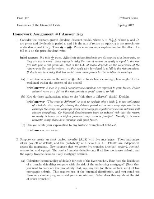
Econ 497<br />
Economics of the Financial Crisis<br />
Professor Ickes<br />
Spring 2012<br />
<strong>Homework</strong> <strong>Assignment</strong> <strong>#1</strong>:<strong>Answer</strong> <strong>Key</strong><br />
1+<br />
1. Consider the constant-growth dividend discount model, where = ,where − and <br />
are prices and dividends in period and istherateofreturnonequity, is the growth rate<br />
of dividends, and .Then <br />
<br />
= 1+ . Provide an economic explanation for the effect of a<br />
−<br />
fall in on the price-dividend ratio.<br />
brief answer If falls <br />
<br />
rises. Effectively future dividends are discounted at a lower rate, so<br />
they are worth more. Since equity is risky the rate of return on equity is equal to the risk<br />
free rate plus a risk premium (that in the CAPM model depends on the covariance of the<br />
return with the market return), so this could also be related to a fall in the risk premium.<br />
If stocks are less risky that too could cause their prices to rise relative to earnings.<br />
(a) If we observe a rise in the ratio of <br />
<br />
relative to its historic average, how might this be<br />
explained within the context of the model?<br />
brief answer Arisein could occur because earnings are expected to grow faster. Faller<br />
interest rates or a fall in the risk premium could cause to fall.<br />
(b) How do these explanations relate to the ”this time is different” thesis? Explain.<br />
brief answer ”Thistimeisdifferent” is used to explain why a high is not indicative<br />
<br />
of a bubble. For example, during the dotcom period prices were very high relative to<br />
earnings the story was earnings would eventually grow faster because the internet will<br />
change everything. Or financial developments have so reduced risk that the return<br />
to equity is lower so a higher price-earnings ratio is justified. Usually it is some<br />
fantastic story about how earnings will grow faster.<br />
(c) Can you relate your explanation to any historic examples of bubbles?<br />
brief answer see above<br />
2. Suppose we create an asset backed security (ABS) with five mortgages. These mortgages<br />
either pay off or default, and the probability of a default is 1. Defaults are independent<br />
across the mortgages. Now suppose that we create five tranches (senior1, senior2, senior3,<br />
mezzanine, andequity). The senior1 tranche defaults only if all five mortgages default, and<br />
the equity tranche defaults if any mortgage defaults.<br />
(a) Calculate the probability of default for each of the five tranches. How does the likelihood<br />
of a tranche defaulting compare with the risk of the underlying mortgages? [Note that<br />
you need to calculate the probability that, say, any two (or three, or four, etc.) of five<br />
mortgages default. This requires use of the binomial distribution, and you could use<br />
Excel or a similar program to aid your computation.]. What does this say about the risk<br />
of senior tranches?<br />
1
ief answer The senior tranche defaults only if all five mortgages default, the senior2<br />
if there are four defaults, and so forth. So we use the cumulative binomial<br />
distribution to calculate the ways that four mortgages default out of five experiments,<br />
then how three can default, etc. For example, the senior1 defaults only if<br />
all five default, so calculate the cumulative probability of only four defaults. Call this<br />
BinomialDist(4; 51) Then 1 − BinomialDist(4; 51) gives the probability of five defaults.<br />
We do this for each tranche. We obtain:<br />
tranche probability of default<br />
senior1<br />
00001<br />
senior2<br />
00046<br />
.<br />
senior3<br />
00856<br />
mezzanine 08146<br />
equity<br />
40951<br />
The senior tranche is obviously very secure. The probability of default is practically<br />
non-existent. The same is true for the senior2 and senior 3, the probability of<br />
default is still very low.<br />
(b) Suppose we now form a new security made up of mezzanine tranches. That is, we combine<br />
five securities with the same probability of default you calculated for the mezzanine<br />
tranche in part a. Call this a Again tranche this new security into five parts with<br />
the same pattern of seniority. Calculate the probability of default of the various tranches<br />
of the <br />
brief answer The probability of default of the mezzanine tranche is 08 So just imagine<br />
we have five bonds with the default probability of this mezzanine trance and form a<br />
new security. It is evident that the default probabilities should fall, since 08 1, that<br />
is the default probability of the mezzanine tranche is less than that of the underlying<br />
mortgage. So with uncorrelated risks, the CDO should be even less risky. That is<br />
what we indeed see. If we tranche it just as in part (a), and perform the same calculation<br />
we obtain:<br />
Default Probability of the CDO of Mezzanine Tranches<br />
tranche probability of default<br />
senior1<br />
000004<br />
senior2<br />
000205<br />
<br />
senior3<br />
004756<br />
mezzanine .056117<br />
equity<br />
345918<br />
We note that the senior tranches still show very low default rates.<br />
(c) Suppose that the probability of default of the underlying mortgages is really 15. How<br />
does this change the probability of the default of the tranches of the ? Howmuch<br />
riskier (say, in percentage terms) does the mezzanine tranche of the get given this<br />
50% increase in the default probability?<br />
brief answer With a higher underlying default probability the default probabilities of<br />
the tranches rise, and the lower tranches somewhat significantly. The default probability<br />
of the mezzanine rises from 08146 to 1648. Sousing1648 in our CDO we get:<br />
2
Default Probability of the CDO of Mezzanine Tranches with .1648 probability of default<br />
tranche probability of default<br />
senior1<br />
00012<br />
senior2<br />
00314<br />
<br />
<br />
senior3<br />
03397<br />
mezzanine .19111<br />
equity<br />
59165<br />
We see that the tranches of the CDO are now riskier that before, essentially by<br />
an order of magnitude. For example, the senior3 tranche had a default probability of<br />
.0047, now it has a default probability of .03397, almost ten times more likely. So the<br />
CDO and CDO 2 are more sensitive to changes in the underlying default probability<br />
than the original ABS is.<br />
(d) What if there were 100 mortgages, 10 to a tranche, and the probability of default of<br />
the underlying loans is 05. Consider tranche10, which defaults if 10 or more mortgages<br />
default. What is the default probability of that tranche? What of the made up of<br />
tranche10 securities? What happens if the underlying probability of default rises to 06?<br />
brief answer The analysis is the same as before. We need to calculate the likelihood<br />
that ten mortgages default out of 100 possibilities. So again use the binomial distribution.<br />
We calculate 1 − BinomialDist(9; 10005) = 002818 8. Now if we form<br />
a CDO made up to tranche10 securities we expect that these will have low default<br />
probabilities, since the default probability of tranche10 is less than that of the underlying<br />
mortgages (028 1). Andindeed,1 − BinomialDist(9; 10002818) = 00054.<br />
But now here is the really interesting part. Suppose that the probability of default<br />
was just a little higher, 06. This is a 20% increase in the risk of the underlying<br />
mortgages. What happens to the default probability of these tranches? We calculate<br />
1 − BinomialDist(9; 10006) = 0775. Notice that the percentage increase in risk of<br />
this tranche is huge: 0775−0281 =%175. For the CDO it is even bigger. We calculate<br />
0281<br />
1 − BinomialDist(9; 1000775) = 02467 which is represents a 2467−00054 = 45339%<br />
00054<br />
increase in risk. That is quite a significant change, so we can conclude that the CDO<br />
tranches are indeed quite sensitive to the underlying default probabilities.<br />
3. Consider the limits to arbitrage model with three types of agents (noise, investors, and arbitragers)<br />
and three periods. In period 3 the value of the asset is , and arbitragers know this<br />
(so 3 = ). Noise traders receive a signal in periods 1 and 2 ( 1 2 ) that may cause them<br />
to be pessimistic. Investors supply funds to arbitragers, and they base their decisions on past<br />
performance. Let the demand for the asset on the part of noise traders be () = − <br />
<br />
at<br />
= 1 abitragers know 1 ,butnot 2 . In particular, there is some chance that 2 1 The<br />
supply of the asset is one for simplicity. Let be the resources available to arbitragers in .<br />
(a) Given that markets clear show that the 2 depends positively on and 2 and negatively<br />
on 2 .Whatdoes 1 depend on? Explain.<br />
brief answer Demand in period 2 from noise traders is − 2<br />
2<br />
, arbitragers want to purchase<br />
as much as they can in period 2, 2<br />
2<br />
, and supply is unity, so 1= − 2<br />
2<br />
+ 2<br />
2<br />
<br />
and thus 2 = − 2 + 2 .Asfor 1 this depends on noise trader demand in period<br />
one, − 1<br />
1<br />
and how much arbitragers will demand. But this is not necessarily equal<br />
3
to 1 , because arbitragers may wait to save some of their gunpowder till period two.<br />
Hence, 1= − 1<br />
1<br />
+ 1<br />
1<br />
,whichimplies 1 = − 1 + 1 .<br />
(b) If arbitragers had access to unlimited funds what will 2 equal?<br />
brief answer If 2 −→ ∞ then arbitragers will offset all noise trader risk and we have<br />
1 = 2 = <br />
(c) Suppose that the supply function of funds to investors is given by<br />
" µ1 2<br />
2 = 1 + #<br />
1 − 1<br />
(1)<br />
1 1 1<br />
(1) = 1 0 ≥ 1 00 ≤ 0<br />
where 1 is the amount invested by arbitragers in period 1, and 0 measures the sensitivity<br />
of 2 to the term in the brackets. If 2 = 1 what happens to 2 ? What happens<br />
if 2 1 ? Explain why this could be important.<br />
brief answer If 2 = 1 then we have 2 = 1 h³ ´ i<br />
1<br />
1<br />
+<br />
1 − 1<br />
1<br />
=⇒ 2 = 1 ,that<br />
is if there is no change in price then funds available are the same. If prices fall,<br />
however, then clearly 2 1 . How much this falls depends on the size of 0 ,the<br />
more sensitive is supply to recent returns the greater the fall. This could be important<br />
because it makes traders reluctant to fully commit to arbitrage possibilities. A shortterm<br />
fluctuation could wipe them out. This makes noise trader sentiment more<br />
important. If fund supply is very sensitive then arbitragers may even have to sell out<br />
in period two, which would move prices even farther from V.<br />
(d) What does 0 0 imply about the nature of arbitrage? Explain. If 0 is larger are<br />
arbitragers more likely to succeed or more likely to fail in offsetting noise traders signals<br />
in period 2?<br />
brief answer When we have PBA then agency intrudes into the arbitrage process. This<br />
means that arbitragers must take into account the possibility that they will lose funds<br />
at the most opportune times for investment. This makes them less willing to commit<br />
their funds and makes it less likely that noise traders are offset.<br />
4


