NE Resilience Report - Conservation Gateway
NE Resilience Report - Conservation Gateway
NE Resilience Report - Conservation Gateway

You also want an ePaper? Increase the reach of your titles
YUMPU automatically turns print PDFs into web optimized ePapers that Google loves.
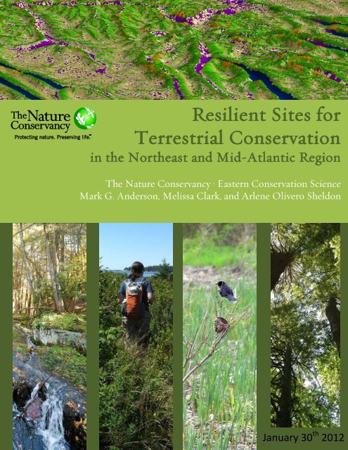
Resilient Sites for<br />
Terrestrial <strong>Conservation</strong><br />
in the Northeast and Mid-Atlantic Region<br />
The Nature Conservancy • Eastern <strong>Conservation</strong> Science<br />
Mark G. Anderson, Melissa Clark, and Arlene Olivero Sheldon<br />
January 30 th 2012
Acknowledgements<br />
This project would not have been possible without the expertise contributed by Brad McRae of<br />
The Nature Conservancy and Brad Compton of University of Massachusetts both who have<br />
created powerful new tools for measuring permeability. They were always willing to listen to our<br />
questions, provide guidance in using the tools correctly, and, in some cases, run the analysis for<br />
us. Charles Ferree also contributed to the mapping and modeling of landforms, and in calculating<br />
the landform variety and elevation range metrics.<br />
We extend warm thanks to Lise Hanners and Barbara Vickery for editing the final report in its<br />
entirety. The report was immensely improved by extensive written comments from Doug<br />
Samson, Judy Duncomb, Barbara Vickery, Lise Hanners, Rodney Bartgis, and Andy Finton, and<br />
verbal comments from many others. We also benefited by review of the final products by<br />
scientists at the Cary Institute and the U.S. Fish and Wildlife Service.<br />
Completing this project took several years; throughout we were guided by an internal team of<br />
Nature Conservancy scientists “the eastern resilience team” who provided assistance with data<br />
gathering, analysis, editing, and review. We would like to thank especially the scientists and<br />
partners in the Central Appalachian region: Judy Dunscomb, Tamara Gagnolet, Thomas Minney,<br />
Angela Watland, Nels Johnson, Rodney Bartgis, Amy Cimarolli, and the Northern Appalachian<br />
region: Barbara Vickery, Mark Zankel, Dirk Bryant, Philip Huffman, Andrew Finton, Megan de<br />
Graaf, Daniel Coker, Louise Gratton, Rebecca Shirer, Rose Paul, Daryl Burtnett, Andrew Cutko,<br />
and Steve Walker. The latter group was instrumental in extending the analysis to Maritime<br />
Canada. Both teams provided critical feedback regarding the results and methodology, and on<br />
the utility of various outputs.<br />
Finally, we would like to thank John Cook, Michael Lipford, and Rodney Bartgis for motivating<br />
this project in the first place and then remaining incredibly patient as we worked out the methods<br />
and tested the analysis. I am sure they watched with dismay as we rejected many more versions<br />
of each analysis than we retained, but we hope the final products prove to be worth the wait.<br />
We are grateful for funding provided by The Doris Duke Charitable Foundation, the Northeast<br />
Association of Fish and Wildlife Agencies, and The Nature Conservancy.<br />
Please cite as:<br />
Anderson, M.G., M. Clark, and A. Olivero Sheldon. 2012. Resilient Sites for<br />
Terrestrial <strong>Conservation</strong> in the Northeast and Mid-Atlantic Region. The Nature<br />
Conservancy, Eastern <strong>Conservation</strong> Science. 168 pp.
Table of Contents<br />
Chapter 1 - Introduction .............................................................................................................................................. 1<br />
Chapter 2 – Defining Sites and Geophysical Settings ........................................................................................... 3<br />
The Sites - 1,000 Acre Hexagons ................................................................................................................ 3<br />
Geophysical Settings ..................................................................................................................................... 3<br />
Grouping Hexagons into Geophysical Settings ............................................................................................ 9<br />
Results ........................................................................................................................................................... 9<br />
Descriptions of the Settings ........................................................................................................................ 11<br />
Low Elevation: Coastal and Very Low Settings ............................................................................ 11<br />
Mid Elevation: Settings from 800’ to 2500’ .................................................................................. 13<br />
High Elevation: Settings over 2500’ .............................................................................................. 14<br />
Chapter 3 – Estimating <strong>Resilience</strong> ............................................................................................................................. 15<br />
Section 1: Landscape Complexity............................................................................................................... 15<br />
Background .................................................................................................................................... 15<br />
Landform Variety........................................................................................................................... 16<br />
Elevation Range ............................................................................................................................. 20<br />
Wetland Density ............................................................................................................................ 20<br />
Landscape Complexity Combined Index ....................................................................................... 24<br />
Section 2: Landscape Permeability ............................................................................................................. 27<br />
Local Connectedness ..................................................................................................................... 28<br />
Species Diversity as a <strong>Resilience</strong> Factor ........................................................................................ 29<br />
Section 3: Combining <strong>Resilience</strong> Factors ................................................................................................... 35<br />
A Common Scale ........................................................................................................................... 35<br />
Landscape Complexity: Integrated Score ...................................................................................... 35<br />
Estimates of <strong>Resilience</strong>: Integrated Score ...................................................................................... 35<br />
Chapter 4 – Regional Linkages .................................................................................................................................. 36<br />
Regional Flow Patterns ............................................................................................................................... 36<br />
Integration with Other Metrics .................................................................................................................... 39<br />
Chapter 5 – Results: Scores for the Settings .......................................................................................................... 41<br />
Sites (1,000 Acre Hexagons) ...................................................................................................................... 42<br />
Individual Geophysical Settings ................................................................................................................. 42<br />
Results by Setting ...................................................................................................................................... 43<br />
Low Elevation Settings .................................................................................................................. 43<br />
Low Elevation Coastal Settings ..................................................................................................... 69<br />
Mid Elevation Settings ................................................................................................................... 77<br />
High Elevation Settings ................................................................................................................. 95
Chapter 6 – Results: Resilient Sites ........................................................................................................................ 110<br />
<strong>Resilience</strong> and Vulnerability ..................................................................................................................... 110<br />
<strong>Resilience</strong> and Geophysical Settings ........................................................................................................ 112<br />
Ecological Regions .................................................................................................................................. 114<br />
Ecoregion Results ..................................................................................................................................... 117<br />
Central Appalachian .................................................................................................................... 120<br />
Chesapeake Bay Lowland ........................................................................................................... 126<br />
High Allegheny Plateau .............................................................................................................. 132<br />
Lower New England – Northern Piedmont ................................................................................. 138<br />
North Atlantic Coast ................................................................................................................... 144<br />
Northern Appalachian - Acadian ................................................................................................ 150<br />
Thirteen-State Region ............................................................................................................................... 156<br />
Composite Map of all Ecoregions ............................................................................................................. 156<br />
Discussion ................................................................................................................................................ 156<br />
Highest scoring areas for estimated resilience ........................................................................... 159<br />
The most resilient examples of each geophysical setting ........................................................... 160<br />
Focal areas with high estimated resilience .................................................................................. 161<br />
Key places of current and future biodiversity ............................................................................ 162<br />
Networks of resilient sites based on linkages and focal areas ..................................................... 163<br />
Securement status of the focal areas ........................................................................................... 164<br />
Highest scoring areas for estimated resilience by setting across the region ............................... 165<br />
Comparison of scores for full region, individual settings and settings within ecoregion ........... 166<br />
References ...................................................................................................................................................................... 167<br />
Appendices ..................................................................................................................................................................... 170<br />
Appendix I: Northern Appalachian-Acadian Foundational Maps ........................................................... 171<br />
Appendix II: Detail on Ecological Land Units ......................................................................................... 178<br />
Appendix III: Detailed Data Sources and Methods .................................................................................. 186<br />
Appendix IV: Species Names used in the <strong>Report</strong> ..................................................................................... 189
CHAPTER<br />
Introduction<br />
1<br />
Climate change is expected to alter species distributions. As species move to adjust to changing<br />
conditions, conservationists urgently require a way to prioritize strategic land conservation that will<br />
conserve the maximum amount of biological diversity despite shifting distribution patterns (IPCC 2007).<br />
Current conservation approaches based on species locations or on predicted species’ responses to climate,<br />
are necessary, but hampered by uncertainty. Here we offer a complementary approach, one that aims to<br />
identify key areas for conservation based on land characteristics that increase diversity and resilience.<br />
The central idea of this project is that by mapping key geophysical settings and evaluating them for<br />
landscape characteristics that buffer against climate effects, we can identify the most resilient places in<br />
the landscape. Ideally, these places will conserve the full spectrum of physical arenas that create and<br />
support species diversity. Additionally, each individual place will offer a range of microclimates and<br />
options for species movement, thus maintaining landscape functionality and improving the chances of<br />
species’ survival in a changing climate. Our approach is based on observations that species diversity is<br />
highly correlated with geophysical diversity in the Northeast and Mid-Atlantic (Anderson and Ferree<br />
2010), that species take advantage of the micro-climates available in complex landscapes, and that species<br />
can move to adjust to climatic changes if the area is permeable. Thus, the characteristics of geophysical<br />
representation, landscape complexity and landscape permeability, are primary concepts in this research.<br />
This report has three basic parts: first, we ensure that all geophysical settings are represented in a<br />
conservation network (Chapter 2); second, we make certain that the sites within a network are selected<br />
for characteristics that increase resilience (Chapter 3); and third, we ensure that the sites are regionally<br />
well connected (Chapter 4). The latter two sections introduce new methodologies to quantify the physical<br />
and structural aspects of the landscape and explain how we identify important linkages between sites. The<br />
metrics developed for estimating site resilience are discussed in the chapters and include models that<br />
measure a site’s physical complexity (landform variety, elevation range, and wetland density) and<br />
permeability (local connectedness and regional flow patterns). Finally, each metric is calculated for a 13-<br />
state U.S. region and the Maritime Provinces of Canada. The results sections of this report (Chapters 5<br />
and 6) identify the network of sites with the highest estimated resilience within each ecological region. As<br />
part of the results, we compare the resilient sites identified in the report with sites previously identified for<br />
their significant biodiversity.<br />
We use the term “resilience” (Gunderson 2000) to refer to the capacity of a site to adapt to climate<br />
change while still maintaining diversity, but we do not assume that the species currently located at these<br />
sites will necessarily be the same species present in a century or two. Instead, we presume that if<br />
conservation succeeds, each setting will support species that thrive in the conditions defined by the<br />
physical setting. For example, low elevation limestone valleys will support species that benefit from<br />
calcium rich soils, alkaline waters, and cave or karst features, while acidic outwash sands will support a<br />
distinctly different set of species. Each geophysical setting, in turn, contains a variety of species habitats<br />
and natural communities. A limestone valley, for example, may contain fens, marshes, and riverine<br />
wetlands, as well as forests, grasslands or barrens on flats or gently sloping dry terrain. These<br />
communities are often associated with the variety of landforms present; our intent was to identify resilient<br />
examples of a geophysical setting that encompass a variety of habitats.<br />
The value of conserving a spectrum of physical settings is based on extensive empirical evidence<br />
(Anderson and Ferree 2010), but there are further conservation choices to make concerning geophysical<br />
representation. For example, out of all the possible low elevation limestone valleys that could be<br />
Resilient Sites for Terrestrial <strong>Conservation</strong> in the Northeast and Mid-Atlantic Region 1<br />
The Nature Conservancy • Eastern <strong>Conservation</strong> Science • Eastern Division • 99 Bedford St • Boston, MA 02111
conserved, which one is the most likely to remain functional and sustain its biological diversity? The<br />
second section of this report focuses specifically on prioritizing among examples of the same setting<br />
using physical characteristics that increase resilience. These characteristics fall into two categories. The<br />
first, landscape complexity, refers to the number of microhabitats and climatic gradients available within<br />
a given area. Complexity is measured by counting the variety of landforms present in a small area, and<br />
modifying that slightly by the elevation range and the density of wetlands. Because topographic diversity<br />
buffers against climatic effects, the persistence of most species within a given area increases in landscapes<br />
with a wide variety of microclimates (Weiss et al. 1988). Landscape permeability, the second factor, is<br />
defined as the number of barriers and degree of fragmentation within a landscape. A highly permeable<br />
landscape promotes resilience by facilitating range shifts and the reorganization of communities. Roads,<br />
development, dams, and other structures create resistance that interrupts or redirects movement and,<br />
therefore, lowers landscape permeability. Maintaining a connected landscape is the most widely cited<br />
strategy in the scientific literature for building resilience (Heller and Zavaleta 2009) and has been<br />
suggested as an explanation for why there were few extinctions during the last period of comparable rapid<br />
climate change, the so-called “Quaternary conundrum” (Botkin et al. 2007).<br />
The report structure follows the structure described in this introduction: representing all geophysical<br />
settings, estimating site resilience and linking sites into networks. The results section presents and<br />
describes the results with respect to individual 1000-acre sites within ecological regions. The ecoregions<br />
have been previously defined by The Nature Conservancy based on the subsections delineated by the U.S.<br />
Forest service and Canadian Provinces (Anderson 1999). Because each region represents an area of<br />
similar physiography and landscape features, it is thus an appropriate natural unit in which to evaluate<br />
geophysical representation and to compare and contrast sites.<br />
Summary: <strong>Resilience</strong> concerns the ability of a living system to adjust to climate change, to moderate<br />
potential damages, to take advantage of opportunities, or to cope with consequences; in short, its capacity<br />
to adapt. In this project we aim to identify the most resilient examples of key geophysical settings (e.g.<br />
sand plains, granite mountains, limestone valleys, etc.) to provide conservationists with a nuanced picture<br />
of the places where conservation is most likely to succeed over centuries. The project had three parts:<br />
1) identifying and mapping the geophysical settings, 2) developing a quantitative estimate of resilience<br />
for each setting based on landscape complexity and permeability, and 3) identifying key linkages that may<br />
be important in facilitating climate-induced regional movements. The final products include the<br />
identification of sites with high or low estimated resilience and overlays of these sites with the TNC<br />
portfolio of important biodiversity sites. The products were presented in an ecoregional context,<br />
highlighting sites with the highest estimated resilience for each setting within each ecoregion.<br />
2 Resilient Sites for Terrestrial <strong>Conservation</strong> in the Northeast and Mid-Atlantic Region<br />
The Nature Conservancy • Eastern <strong>Conservation</strong> Science • Eastern Division • 99 Bedford St • Boston, MA 02111
CHAPTER<br />
Defining Sites and<br />
2<br />
Geophysical Settings<br />
This section describes the process of characterizing local landscapes (sites) and classifying them into<br />
distinct geophysical settings. Although the settings were defined by physical characteristics, they differ in<br />
the flora and fauna they support, and in their inherent resilience; the latter differences reflecting both<br />
historical management and ecological character. A classification enabled us to compare resilience<br />
characteristics among sites that represent similar geophysical settings. For example, the region’s high<br />
granite mountains are both largely intact and topographically complex, whereas low coastal sandplains<br />
are both highly fragmented and relatively flat. By comparing characteristics among sites of the same type<br />
(e.g. among all low coastal sandplain sites) we could identify the most resilient examples of each setting,<br />
recognizing that some settings are inherently more vulnerable than others.<br />
Our choice of classification factors was guided by previous work to understand the physical factors that<br />
underlie the region’s biodiversity patterns. Specifically, geology classes and elevations zones follow those<br />
described in Anderson and Ferree (2010) and found to be tightly correlated with species diversity patterns<br />
in this region. (see: http://www.plosone.org/article/info%3Adoi%2F10.1371%2Fjournal.pone.0011554)<br />
The Sites - 1,000 Acre Hexagons: Our primary unit of analysis was a 1,000-acre hexagon. We chose this<br />
unit because the size allowed assessment of relatively fine-scale detail, and because the hexagon shapes<br />
match edge-to-edge to perfectly tessellate the entire landscape – like a soccer ball. The entire 13-state<br />
region subdivides into 156,581 hexagons and we calculated the variables described below for each one,<br />
plus the three Canadian Maritime Provinces and the lower portion of Quebec. Additionally, the size of the<br />
unit allowed us to maintain the sensitivity of the exact location of the rare species (“element<br />
occurrences”) and allowed for some spatial error in those locations. We refer to each hexagon as a “site”<br />
but in later sections the individual hexagons aggregate to form larger “conservation areas,” or larger<br />
patches of the setting. The full extent of each setting in the region is the sum of all the variously-sized<br />
patches and sites that share the same physical characteristics.<br />
We attributed each hexagon with basic information about its land and water features, its geographic<br />
context, and the species and communities it currently contains. The attributes ranged from simple location<br />
information, such as the state and ecoregion that contained the hexagon, to the specific geophysical<br />
characteristics described below. Note that some of the analyses described later in this report were done at<br />
finer or coarser scales, and these were then summarized to the hexagon scale – see figure 5.1 in Chapter<br />
5 for an illustration.<br />
Geophysical Settings: Information on geology, elevation, and landforms was used to characterize the<br />
physical attributes of each hexagon, and these attributes were used to identify sets of hexagons that<br />
represent the same geophysical setting. Throughout this report, we use descriptive terms to refer to these<br />
characteristics, but each one was mapped using carefully defined quantitative criteria. For example, what<br />
we descriptively call a flat summit (the level top of a mountain or ridge) is defined in mapping terms as a<br />
landform with 0-2 degrees slope, found in the highest land position. We provide maps and illustrations to<br />
Resilient Sites for Terrestrial <strong>Conservation</strong> in the Northeast and Mid-Atlantic Region 3<br />
The Nature Conservancy • Eastern <strong>Conservation</strong> Science • Eastern Division • 99 Bedford St • Boston, MA 02111
help users understand how the characteristics lay out on the landscape and further explanation of the<br />
landform model is given in Chapter 4. Additionally, greater detail about the process of defining and<br />
mapping each attribute is provided in Appendix II and in Anderson (1999) and Anderson and Ferree<br />
(2010).<br />
The geophysical categories used to define the setting were:<br />
Elevation Zones (Map 3.1)<br />
These zones correspond to major changed in vegetation patterns (see Anderson 1999)<br />
Low: 0’ to 800’ elevation, includes coastal (0-20’) and very low oak-pine zones<br />
Mid: 800’ to 2500’ elevation, includes current northern hardwood and transition zones<br />
High: 2500’ to 3600’+, includes current spruce-fir and alpine zones<br />
Geology Classes (Map 3.2)<br />
To create a regional geology map, the state and provincial digitized geological maps were compiled and<br />
synthesized; the large array of individual bedrock and surficial sediment types were grouped into one of<br />
these major classes. The nine categories were based on the chemical and physical properties of the soils<br />
derived from them, and are correlated with regional biodiversity patterns (see Anderson and Ferree 2010<br />
and appendix for full listing).<br />
Acidic sedimentary: Fine to coarse-grained, acidic sedimentary or meta-sedimentary rock, this group<br />
included: mudstone, claystone, siltstone, non-fissile shale, sandstone, conglomerate, breccia, greywacke,<br />
and arenites. Metamorphic equivalents: slates, phyllites, pelites, schists, pelitic schists, granofels.<br />
Acidic shale: This group included any fine-grained loosely compacted acidic fissile shale.<br />
Calcareous: Alkaline, soft, sedimentary or metasedimentary rock with high calcium content, this group<br />
included: limestone, dolomite, dolostone, marble, other carbonate-rich clastic rocks.<br />
Moderately Calcareous: Neutral to alkaline, moderately soft sedimentary or meta-sedimentary rock with<br />
some calcium but less so than the calcareous rocks, this group included: calcareous shales, pelites and<br />
siltstones, calcareous sandstones, lightly metamorphosed calcareous pelites, quartzites, schists and<br />
phyllites, calc-silicate granofels.<br />
Acidic Granitic: Quartz-rich, resistant acidic igneous and high grade meta-sedimentary rock, this group<br />
includes: granite, granodiorite, rhyolite, felsite, pegmatite, granitic gneiss, charnockites, migmatites,<br />
quartzose gneiss, quartzite, quartz granofel.<br />
Mafic: Quartz-poor alkaline to slightly acidic rock, this group includes: (ultrabasic) anorthosite (basic),<br />
gabbro, diabase, basalt (intermediate), quartz-poor: diorite/ andesite, syenite/ trachyte, greenstone,<br />
amphibolite, epidiorite, granulite, bostonite, essexite.<br />
Ultramafic: Magnesium-rich alkaline rock, this group includes: serpentine, soapstone, pyroxenites,<br />
dunites, peridotites, talc schist.<br />
Coarse Surficial Sediment: This group includes deep unconsolidated sand and gravel.<br />
Fine Surficial Sediment: This group includes deep unconsolidated silt and mud.<br />
4 Resilient Sites for Terrestrial <strong>Conservation</strong> in the Northeast and Mid-Atlantic Region<br />
The Nature Conservancy • Eastern <strong>Conservation</strong> Science • Eastern Division • 99 Bedford St • Boston, MA 02111
Landform Types (Map 3.3)<br />
The landform modeling is described in detail in Chapter 4.1 and in Appendix II, and images of how each<br />
mapped type fit within a landscape are provided. Although any numbers of landforms can be delineated,<br />
we used an eleven-unit model:<br />
1) Cliff/steep slope (includes cliffs, and steep slopes of warm and cool aspects)<br />
2) Summit/ridgetop (includes flat summit, upper ridges, and slope crests)<br />
3) Northeast sideslope (includes moderately steep sideslopes of cooler aspects)<br />
4) Southwest sideslope (includes moderately steep sideslopes of warmer aspects)<br />
5) Cove/slope bottom (includes slope bottom flats, and coves of warm and cool aspects)<br />
6) Low hill<br />
7) Low hilltop flat<br />
8) Valley/toeslope<br />
9) Dry flat<br />
10) Wet flat<br />
11) Water (includes lakes, ponds, rivers and estuaries)<br />
Species and Natural Community Information<br />
Each geophysical setting supports a variety of species habitats and natural communities. A limestone<br />
valley, for example, may contain fens, marshes, and riverine wetlands associated with wet flats and<br />
streams, as well as forests, grasslands, and barrens associated with flats or gently sloping dry terrain. The<br />
variety of landforms present often determines the variety of communities and habitats. To quantify the<br />
types of species and communities currently found in each setting we overlaid locations of rare species and<br />
exemplary natural communities tracked and inventoried by the State Natural Heritage field inventory<br />
programs. Sensitive locations were used with permission, and are not available for redistribution. For the<br />
overlays, all source occurrence datasets (points and polygons) were converted to point features based on<br />
the polygon’s centroid. Point location with adequate precision to overlay with 1,000 acre hexagons were<br />
then tagged with the identification of the hexagon in which they fell. If multiple occurrences of the same<br />
species or community fell in the same hexagon, the number of occurrences was recorded, but the<br />
attributes of the hexagon were only counted once for that feature. The results of the species overlays are<br />
included in Appendix III along with more details on the mapping and overlay of the species known<br />
locations. The results of the community overlays are included in the descriptions of each setting because,<br />
although we expect the composition of these communities to rearrange, they give a clear idea of the types<br />
of ecosystems that the setting supports and will likely remain present in some future form.<br />
Resilient Sites for Terrestrial <strong>Conservation</strong> in the Northeast and Mid-Atlantic Region 5<br />
The Nature Conservancy • Eastern <strong>Conservation</strong> Science • Eastern Division • 99 Bedford St • Boston, MA 02111
Map 3.1: Elevation zones. The three zones are further subdivided into six on this map.<br />
6 Resilient Sites for Terrestrial <strong>Conservation</strong> in the Northeast and Mid-Atlantic Region<br />
The Nature Conservancy • Eastern <strong>Conservation</strong> Science • Eastern Division • 99 Bedford St • Boston, MA 02111
Map 3.2: The nine geology classes used in this report.<br />
Resilient Sites for Terrestrial <strong>Conservation</strong> in the Northeast and Mid-Atlantic Region 7<br />
The Nature Conservancy • Eastern <strong>Conservation</strong> Science • Eastern Division • 99 Bedford St • Boston, MA 02111
Map 3.3: Landform types. Note that in this map some of the eleven basic landform types are further<br />
subdivided by aspect or location (see text) .<br />
8 Resilient Sites for Terrestrial <strong>Conservation</strong> in the Northeast and Mid-Atlantic Region<br />
The Nature Conservancy • Eastern <strong>Conservation</strong> Science • Eastern Division • 99 Bedford St • Boston, MA 02111
Grouping Hexagons into Geophysical Settings: We tabulated the abundance and percentage of each<br />
physical element described above for each hexagon, and this information formed the basis for measuring<br />
similarity among hexagons. Specifically, we classified all hexagons into geophysical settings based on<br />
their geological composition (nine classes) and elevation zones (three classes); potentially 27 distinct<br />
settings (e.g. low elevation granite). First, we identified and tagged all the homogenous hexagons<br />
composed 80 percent or more of a single elevation zone and single geologic class. Second, we used a<br />
cluster analysis to assign the hexagons with more heterogeneous compositions into the most similar<br />
setting based on elevation, geology and landform.<br />
For example, a single hexagon, classified as high elevation granite, might be composed of:<br />
90 percent high elevation granite<br />
10 percent high elevation mafic<br />
50 percent side slopes<br />
35 percent steep slopes<br />
15 percent summits<br />
5 percent wet flat<br />
0 percent all other attributes<br />
The above example could be assigned to a group by a simple query of attribute values and applying the 80<br />
percent criteria, and this method worked for the vast majority of hexagons. For more heterogeneous<br />
hexagons we used quantitative clustering to determine which geophysical group the unclassified had the<br />
most attributes in common with. Clustering was performed using a hierarchical cluster analysis (PCORD,<br />
McCune and Grace 2002) using the Sorenson similarity index applied to the geophysical attributes<br />
(including landforms), using a flexible beta linkage technique with Beta set at ¬25 (McCune and Grace<br />
2002). After clustering the samples, we performed an indicator species analysis (Dufrene and Legendre<br />
1997) to identify the geophysical attributes that were the most faithful and exclusive to each setting.<br />
Because of the large size of the dataset, much of the clustering was performed in batches. The classified<br />
hexagons were then rejoined with the main coverage to create a single unified coverage.<br />
Results: The results indicated that one of the potential 27 settings did not occur in the region (i.e.. high<br />
elevation ultramafic); however, four other distinct settings were identified that consisted of intermixed<br />
complexes of two settings (low elevation granite and coarse sand) or extreme landforms (extremely steep<br />
slopes). In the end, we recognized 30 distinct geophysical settings, and assigned each of the 150,000+<br />
hexagons into one of them. The settings are described and mapped below (Map 3.4), and evaluated in<br />
chapter 5. They included 15 low elevation settings, 8 mid elevation settings, 6 high elevation setting and 1<br />
miscellaneous high slope setting.<br />
Resilient Sites for Terrestrial <strong>Conservation</strong> in the Northeast and Mid-Atlantic Region 9<br />
The Nature Conservancy • Eastern <strong>Conservation</strong> Science • Eastern Division • 99 Bedford St • Boston, MA 02111
Map 3.4: Geophysical Settings used in this <strong>Report</strong>. The settings are combinations of an elevation zone<br />
and a geology class such as “low elevation calcareous” (L:CALC). See Appendix I for the corresponding<br />
map showing Maritime Canada and the full Northern Appalachian-Acadian extent.<br />
10 Resilient Sites for Terrestrial <strong>Conservation</strong> in the Northeast and Mid-Atlantic Region<br />
The Nature Conservancy • Eastern <strong>Conservation</strong> Science • Eastern Division • 99 Bedford St • Boston, MA 02111
Descriptions of the Settings.<br />
The descriptions are organized by three broad elevation zones, and the number of settings decreases with<br />
increasing elevation. Information on the species and communities that are currently located in the setting<br />
are based on Natural Heritage occurrences, and are provided to give users an indication of the type of<br />
biodiversity that this setting favors. We do not expect these species or communities to occur in these<br />
settings in all parts of the region or to stay the same in the future, but we do expect the future composition<br />
to be of a similar character.<br />
LOW ELEVATION: Coastal and Very Low Elevation Settings.<br />
Settings below 800’ including coastal plains, large floodplains, river mouths and deltas, coastal<br />
shorelines, beaches and dunes, tidal marshes and other low elevation settings.<br />
Rare species currently found across most of these settings includes the following: Vertebrates:<br />
Cooper's hawk, grasshopper sparrow, pied-billed grebe, red-headed woodpecker, sharp-shinned hawk,<br />
yellow-breasted chat, american bittern, bobolink, long-eared owl, red-shouldered hawk, vesper<br />
sparrow, yellow rail, upland sandpiper, black tern, eastern meadowlark, common nighthawk, brown<br />
thrasher, spotted turtle, carpenter frog, tiger salamander, New England cottontail, glassy darter.<br />
Invertebrates: eastern lampmussel, eastern pond mussel, fragile papershell, tidewater mucket, yellow<br />
lampmussel, glassy darter<br />
Geophysical Settings in the Low Elevation Group<br />
Non-coastal settings: the non-coastal low elevation settings occur above 20’ and below 800’, these are<br />
the most abundant and widespread environments in the region.<br />
Low Elevation Coarse Sand (L-COARSE): Coastal plain settings with oak-pine forest, pine barrens,<br />
coastal plain ponds. Numerous rarities.<br />
Low Elevation Granite (L-GRAN): Rocky bedrock-based acidic setting with hilltop woodlands.<br />
Low Elevation Mixed Granite and Coarse Sand (L-GRAN/COARSE): A common setting supporting<br />
acidic forests, inland dunes, and many rarities.<br />
Low Elevation Fine Silt (L-FI<strong>NE</strong>): Fertile silt or clay setting in old lake beds and floodplains.<br />
Low Elevation Mafic (L-MAFIC): Setting on volcanic basalts, or other mafic rocks such as trap rock<br />
ridges or old ring dikes; often with a richer flora and fauna than the more acidic settings.<br />
Low Elevation Acidic Sedimentary (L-SED): Widespread settings on sandstone, siltstone, conglomerate<br />
usually overlain with shallow till and supporting many common acidic forests types.<br />
Low Elevation Sedimentary and Coarse Sand (L-SED/COARSE): Uncommon setting characterized by<br />
river bluffs, shoreline marshes, dry forests and acidic wetlands.<br />
Low Elevation Calcareous (L-CALC): Fertile agricultural and timber lands on limestone and dolomite<br />
that support an array of distinctive communities and rare species.<br />
Resilient Sites for Terrestrial <strong>Conservation</strong> in the Northeast and Mid-Atlantic Region 11<br />
The Nature Conservancy • Eastern <strong>Conservation</strong> Science • Eastern Division • 99 Bedford St • Boston, MA 02111
Low Elevation Moderately Calcareous (L-MODCALC): Fertile settings similar to calcareous but less<br />
distinctive and slightly more common. Bedrock is a mixture of acidic and calcareous rock.<br />
Low Elevation Granitic and Calcareous (L-GRAN/CALC): Mixed settings with pockets of limestone<br />
communities embedded in an acidic granitic matrix.<br />
Low Elevation Acidic Shale (L-SHALE): Settings on unstable shale slopes often supporting a unique<br />
flora and sedimentary-like shale lowlands.<br />
Low Elevation Ultramafic (L-ULTRA): Settings on toxic soils high in nickel and chromium supporting<br />
stunted trees and a unique flora.<br />
Coastal settings: we present the information on the coastal zone for completeness and interest; however,<br />
the methods presented here have numerous problems in the coastal zone. Foremost among these, is that<br />
the data sets are inconsistent in their coastal boundaries and most of the coastal hexagons extend into the<br />
“ocean” outside of this analysis. Thus, the generated numbers and calculations for these settings are<br />
not trustworthy and the results may be misleading. On the settings maps (Map 3.4), these three<br />
settings can be seen as to fringe the coastal boundary.<br />
Coastal Bedrock Settings (L-COAST/BED): Maritime settings under 20’ elevation where bedrock of<br />
any type predominates. Forests and swamps.<br />
Coastal Coarse Sand (L-COAST/COARSE): Maritime settings under 20’ elevation on coarse sand.<br />
Beaches, dunes, swales and sandplains.<br />
Coastal Fine Silt (L-FI<strong>NE</strong>): Maritime settings under 20’ elevation on fine silts and mud. Coastal tidal<br />
marshes, salt marsh, river mouths, swamps.<br />
12 Resilient Sites for Terrestrial <strong>Conservation</strong> in the Northeast and Mid-Atlantic Region<br />
The Nature Conservancy • Eastern <strong>Conservation</strong> Science • Eastern Division • 99 Bedford St • Boston, MA 02111
Mid Elevation: Settings from 800’ to 2500’.<br />
Communities in this elevation zone that are inventoried and monitored by the State Natural<br />
Heritage Programs: boreal conifer swamp, limestone / dolomite barren, acidic shrub swamp,<br />
ridgetop dwarf-tree forest, high-energy riverbank community, allegheny oak forest,<br />
broadleaf-conifer swamp, maple-basswood rich mesic forest, boreal acidic cliff, hemlock<br />
forest. intermediate fen, montane dry calcareous forest, northern new england calcareous<br />
seepage swamp, rich hemlock-hardwood peat swamp, spruce-fir swamp, glacial bog,<br />
hemlock palustrine forest, hillside graminoid-forb fen, ice cave talus community, mountain<br />
acidic woodland, mountain acidic seepage swamp, seepage forest, acidic rocky summit/rock<br />
outcrop community, spruce flats, acidic talus slope woodland.<br />
Rare Species in this elevation zone that are inventoried and monitored by the State Natural<br />
Heritage Programs: Vertebrates: Shenandoah salamander, West Virginia spring salamander,<br />
peregrine falcon, golden eagle, blackpoll warbler,yellow-bellied flycatcher, bluebreast darter,<br />
spotted darter, Tippecanoe darter, rock vole, eastern massasauga, timber rattlesnake,<br />
Invertebrates: Franz's cave isopod, Henrot's cave isopod, Elk River crayfish, Helma's netspinning<br />
caddisfly, Harris's checkerspot, rubifera dart, New England bluet, yellow lance,<br />
northern riffleshell, snuffbox, Atlantic pigtoe, longsolid, clubshell, round pigtoe, Plants:<br />
northern monk's-hood, musk root, shale barren rockcress, Bartram shadbush, piratebush, blue<br />
ridge bittercress, Hammond's yellow spring beauty, Schweinitz' sedge, spreading pogonia,<br />
blunt manna-grass, auricled twayblade, drooping bluegrass<br />
Geophysical Settings in the Mid Elevation Group<br />
These are settings that occur above 800’ and below 2500’.<br />
Mid Elevation Granite (M-GRAN): Mountainous settings supporting natural communities typical of<br />
acid nutrient-poor shallow-soil environments<br />
Mid Elevation Mafic (M-MAFIC): Mountainous settings often intermixed with granite, but derived from<br />
volcanic basalts or intrusive igneous rocks, and supporting a richer flora and fauna.<br />
Mid Elevation Acidic Sedimentary (M-SED): Resistant ridges and high plateaus composed of<br />
sandstone, siltstone, or conglomerates. This abundant setting supports many common acidic forests types.<br />
Mid Elevation Calcareous (M-CALC): Fertile rolling settings on limestone and dolomite that support an<br />
array of distinctive communities including caves, alkaline wetlands and limestone barrens.<br />
Mid Elevation Moderately Calcareous (M-MODCALC): Fertile settings similar to calcareous, but less<br />
distinctive and slightly more common. Bedrock is a mixture of acidic and calcareous rock.<br />
Mid elevation Acidic Shale (M-SHALE): Settings on unstable shale slopes often supporting a unique<br />
flora and sedimentary-like shale lowlands<br />
Mid Elevation Surficial Sediments (M-SURF): Valley or flat settings with surficial deposits of sand or<br />
silt: floodplains and shorelines.<br />
Mid elevation Ultramafic (M-ULTRA): Very rare settings on toxic serpentine soils high in nickel and<br />
chromium supporting stunted trees and a unique flora.<br />
Resilient Sites for Terrestrial <strong>Conservation</strong> in the Northeast and Mid-Atlantic Region 13<br />
The Nature Conservancy • Eastern <strong>Conservation</strong> Science • Eastern Division • 99 Bedford St • Boston, MA 02111
High Elevation: Settings over 2500’.<br />
Communities in the elevation zone that are inventoried and monitored by the State Natural Heritage<br />
Programs: alpine krummholz, alpine peatland, grass bald, montane yellow birch-red spruce forest,<br />
montane spruce-fir forest, mountain fir forest, mountain peatland, high-elevation seepage swamp, highelevation<br />
cove forest, northeast boreal heathland, northeast moist subalpine heathland, northern new<br />
england cold-air talus, red spruce-fraser fir /southern mt cranberry forest, red spruce / great laurel<br />
forest.<br />
Rare Species in this elevation zone of that are inventoried and monitored by the State Natural Heritage<br />
Programs: Vertebrates: Cheat Mountain salamander, Cow Knob salamander, Peaks of Otter<br />
salamander , Bicknell's thrush, candy darter, cheat minnow, Virginia northern flying squirrel, southern<br />
rock vole, southern water shrew, virginia big-eared bat, Invertebrates: White Mountain fritillary,<br />
hudsonian whiteface, bog copper, White Mountain butterfly, Katahdin arctic, Spruce Knob threetooth,<br />
Plants: bog rosemary,dwarf white birch, sand-heather, long-stalked holly, Marcescent sandwort,<br />
Robbins' cinquefoil, northern meadow-sweet, small cranberry.<br />
High Elevation Granite or Mafic (H-GRAN): Bedrock mountain setting of intrusive granitic rock,<br />
plutons of mafic rock or volcanic basalts.<br />
High Elevation Sedimentary (H-SED): Bedrock mountain setting of sandstone, quartzite, conglomerate<br />
or other resistant sedimentary rocks .<br />
High Elevation Mixed Sedimentary and Calcareous (H-SED/CALC): Mountains and ridges of<br />
resistant sandstone intermixed with valleys or lowlands of limestone or other calcareous bedrock.<br />
High Elevation Calcareous and Moderately Calcareous (H-CALC/MOD): Mountainous landscapes of<br />
rich limestone or dolomite.<br />
High Elevation Acidic Shale (L-SHALE): Settings on stable and unstable shale slopes.<br />
Alpine and Subalpine (ALP-ALL): Very high elevation settings over 2500’ on any substrate with<br />
systems dominated by extreme wind and cold. Alpine areas often have stunted trees (krumholz) and<br />
unique floras.<br />
14 Resilient Sites for Terrestrial <strong>Conservation</strong> in the Northeast and Mid-Atlantic Region<br />
The Nature Conservancy • Eastern <strong>Conservation</strong> Science • Eastern Division • 99 Bedford St • Boston, MA 02111
CHAPTER<br />
Estimating <strong>Resilience</strong><br />
3<br />
A central premise of this report is that the physical characteristics of a landscape can buffer an area from<br />
the direct effects of a changing climate by offering a connected array of microclimates that allow species<br />
to persist. We call this quality the site’s adaptive capacity, or its resilience. In this section we describe the<br />
concepts, methods, and data used to estimate the relative resilience of any given site. The two factors<br />
important to the estimate - landscape complexity and landscape permeability – are discussed separately,<br />
because the tools for assessing and measuring them are distinctly different.<br />
Section 1: Landscape Complexity<br />
Background: The actual climate experienced by an individual organism at a given point on the ground<br />
may differ dramatically from the regional norm because the land’s surface features break up climate into a<br />
variety of microclimates influenced by landforms like hills, hollows, and water bodies. As the climate<br />
changes, these microclimates offer options to resident species, and in response to climatic changes,<br />
species are likely to shift their locations slightly to take advantage of this variation and stay within their<br />
preferred temperature and moisture regimes. Thus, the variety of microclimates present in a landscape,<br />
what we term the site’s landscape complexity, can be used to estimate the capacity of the site to maintain<br />
species and functions. We measured landscape complexity as a function of topography, elevation range,<br />
and moisture gradients.<br />
Topography describes the natural surface features of an area, and these natural features can be grouped<br />
into local units known as landforms (e.g. cliffs, summits, coves, basins, valleys). Landforms are a primary<br />
edaphic controller of species distributions, even without climatic considerations, due to the variation in<br />
rates of erosion and deposition, in soil depth and texture, in nutrient availability, and in the distribution of<br />
moisture. Each landform, then, represents a local expression of solar radiation, soil development, and<br />
moisture availability; a variety of landforms results in a variety of meso and micro climates. When<br />
climate is considered, landform variation increases the persistence of species and buffers against direct<br />
climate effects by providing many combinations of temperature and moisture within a local<br />
neighborhood.<br />
Researchers have documented how topographic variation can create surprisingly large temperature ranges<br />
in close proximity. For example, in South Carolina’s Blue Ridge Mountains south-facing slopes were<br />
measured at 104 0 in July, while a few hundred yards away the sheltered ravines were a cool 79 0 (P.<br />
McMillan, personal communication, October 2010). Weiss et al. (1988) measured micro-topographic<br />
thermal climates in relation to butterfly species and their host plants, and concluded that areas of high<br />
local landscape complexity, even on a scale of tens of meters, appear particularly important for long-term<br />
population persistence under variable climatic conditions. Extinctions predicted from coarse-scale climate<br />
envelope models have recently come into question because many current models fail to capture the effects<br />
of topographic and elevation diversity in creating “microclimatic buffering” (Willis and Bhagwat 2009).<br />
For example, Randin et al. (2008) found that models predicting the loss of all suitable habitats for plants<br />
in the Swiss Alps conversely predicted the persistence of suitable habitats for all species when they were<br />
rerun at local scales that captured topographic diversity. Similarly, a model that included topographic<br />
diversity and elevation range predicted only half the species loss of butterflies in a mountainous area<br />
compared to a model based solely on climate (Luato and Heikkinen 2008).<br />
Resilient Sites for Terrestrial <strong>Conservation</strong> in the Northeast and Mid-Atlantic Region 15<br />
The Nature Conservancy • Eastern <strong>Conservation</strong> Science • Eastern Division • 99 Bedford St • Boston, MA 02111
We hypothesized that sites with a large variety of landforms and long elevation gradients will retain more<br />
species throughout a changing climate by offering ample microclimates and thus more options for<br />
rearrangement. However, we found that in areas with very little topographic diversity, we needed a finerscale<br />
indicator of subtle micro topographic features, to distinguish between otherwise similar landscapes.<br />
We chose wetland density as a surrogate for micro-topography in flat landscapes after experimenting with<br />
several rugosity measures. Our final measure of landscape complexity was based on landform variety,<br />
elevation range and, in flats, wetland density. Below we describe how we measured each of these<br />
landscape elements.<br />
Landform Variety: To be explicit about the number of microclimatic settings created by an area’s surface<br />
features we created a landform model that delineated local environments with distinct combinations of<br />
moisture, radiant energy, deposition, and erosion. The model, based on Ruhe and Walker’s (1968) fivepart<br />
hillslope model of soil formation, and Conacher and Darymple’s (1977) nine-unit land surface model,<br />
categorizes various combinations of slope, land position, aspect, and moisture accumulation (Figure 3.1<br />
and 3.2). The methods to develop the model were based on Fels and Matson (1997) and are described in<br />
Anderson (1999) and in Appendix II. The major divisions are based on relative land position and slope<br />
(Figure 3.3) with side slopes further subdivided by aspect, and flats further subdivided by flow<br />
accumulation. The landform model can distinguish an unlimited number of landform units, but we used a<br />
simple 11 unit model that captures the major differences in settings and combines some landform types<br />
that typically occur as pairs (e.g. cliff/steep slope, cove/slope bottom) so they did not skew the results.<br />
The types include the following (Figure 3.1-3.3):<br />
Cliff/steep slope<br />
Summit/ridgetop<br />
<strong>NE</strong> sideslope<br />
SE sideslope<br />
Cove/slope bottom,<br />
Low hill<br />
Low hilltop flat<br />
Valley/toeslope<br />
Dry flat<br />
Wet flat<br />
Water/lake/river<br />
To calculate the landform variety metric we tabulated the number of landforms within a 100-acre circle<br />
around every 30-meter cell in the region using a focal variety analysis on the 11 landform types. Scores<br />
for each cell ranged from 1 to 11 (Map 3.1, Figure 3.4 a. & b.) with a mean of 6.05 and a standard<br />
deviation of 1.85.<br />
With respect to climate change, our assumption was that separate landform settings will retain their<br />
distinct processes despite a changing climate. For example, a hot dry eroding upper slope will continue to<br />
offer a climatic environment different from a cool moist accumulating toe slope.<br />
16 Resilient Sites for Terrestrial <strong>Conservation</strong> in the Northeast and Mid-Atlantic Region<br />
The Nature Conservancy • Eastern <strong>Conservation</strong> Science • Eastern Division • 99 Bedford St • Boston, MA 02111
Figure 3.1: Topographic position and basic relationship to community types. The diversity of<br />
landforms within certain geologic settings leads to distinct expressions of biological diversity.<br />
Physical Diversity<br />
Landforms<br />
Flat<br />
Summit<br />
Granitic<br />
Cliff<br />
Cliff<br />
Steep Slope<br />
Sideslope<br />
River<br />
Rounded<br />
Summit<br />
Sideslope<br />
Slope<br />
Bottom<br />
Flat<br />
Upper Slope<br />
Steep<br />
Slope<br />
Slope Crest<br />
<strong>NE</strong> Facing<br />
Sideslope<br />
Sedimentary<br />
Cove Toe Slope<br />
Dry Flat<br />
Stream<br />
Sedimentary<br />
Wet Flat<br />
Dry Flat on Fine<br />
Sediment<br />
Dry Flat on<br />
Coarse Sediment<br />
River<br />
Physical Diversity<br />
Biological Diversity<br />
Red Spruce<br />
Woodland<br />
Oak-Hickory<br />
Woodland<br />
Northern<br />
Hardwoods<br />
Sparse<br />
Acidic Cliff<br />
Northern<br />
Hardwoods<br />
Rich Northern<br />
Hardwoods<br />
Spruce-Fir-<br />
Tamarack<br />
Swamp<br />
White Pine -<br />
Northern<br />
Hardwood<br />
Forest<br />
Black Spruce<br />
Peatland<br />
Cedar<br />
Swamp<br />
Cattail<br />
Marsh<br />
Calcareous Ultramafic Acidic Granitic Acidic Sedimentary<br />
Resilient Sites for Terrestrial <strong>Conservation</strong> in the Northeast and Mid-Atlantic Region 17<br />
The Nature Conservancy • Eastern <strong>Conservation</strong> Science • Eastern Division • 99 Bedford St • Boston, MA 02111
Figure 3.2: An 11-unit landform model mapped for Mount Mansfield, VT. This graphic shows how<br />
the landforms lie across on the landscape.<br />
18 Resilient Sites for Terrestrial <strong>Conservation</strong> in the Northeast and Mid-Atlantic Region<br />
The Nature Conservancy • Eastern <strong>Conservation</strong> Science • Eastern Division • 99 Bedford St • Boston, MA 02111
Figure 3.3: The underlying slope and land position model used to create the mapped landform<br />
grids. Adapted from Fels and Matson 1997<br />
Resilient Sites for Terrestrial <strong>Conservation</strong> in the Northeast and Mid-Atlantic Region 19<br />
The Nature Conservancy • Eastern <strong>Conservation</strong> Science • Eastern Division • 99 Bedford St • Boston, MA 02111
The landform model describes major difference in local climatic settings, but it is theoretically possible to<br />
detect smaller gradations in topography, or to distinguish between settings that have the same landform<br />
diversity, but longer or shorter elevation gradients. We experimented with a variety of ways to measure<br />
these nuances and settled on the two described below after comparing the results at known sites and<br />
talking with practitioners about the results.<br />
Elevation Range: Species distributions may increase or decrease in elevation in concert with climate<br />
changes, particularly in hilly and mountainous landscape where the effects of elevation are magnified by<br />
slope. In flat landscapes, small elevation changes may have a dramatic effect on hydrologic processes<br />
such as flooding. To measure local elevation range we created an elevation range index by compiling a<br />
30-meter digital elevation model for the region (USGS 2002) and using a focal range analysis to tabulate<br />
the range in elevation within a 100-acre circle around each cell. Scores for each cell ranged from 1 to 795<br />
meters (Map 3.2, Figure 3.4 c) with a mean of 59.4 m and a standard deviation of 54.3. The data were<br />
highly skewed towards zero and were log transformed for further analysis (mean 3.64 and standard<br />
deviation of 1.08).<br />
Wetland Density: A large part of this region is flat and wet, the result of past glaciations. Moreover,<br />
climate models disagree on whether the region will get wetter or drier, or both. In these flat areas,<br />
landform variety is low, elevation change is minimal, and wetlands are extensive. Visual examination of<br />
the landform variety and elevation range maps described above suggested that this information alone did<br />
not always provide enough separation between sites, with respect to the long term resilience of extensive<br />
wetland areas. Further, modeled measures of moisture accumulations had the highest rates of error in<br />
extremely flat landscapes. After experimentation with local rugosity measures, we determined that<br />
directly measuring wetland density provided the best available gauge of small and micro-scale<br />
topographic diversity and patterns of freshwater accumulation. We assumed that areas with high density<br />
of wetlands had higher topographic variation, and therefore offered more options to species, and that<br />
small isolated wetlands were more vulnerable to shrinkage and disappearance than wetlands embedded in<br />
a landscape crowded with other wetlands. Thus, our hypothesis was that wetland dependent species and<br />
communities would be more resilient in a landscape where there was a higher density of wetland features<br />
corresponding to more opportunities for suitable habitat nearby.<br />
20 Resilient Sites for Terrestrial <strong>Conservation</strong> in the Northeast and Mid-Atlantic Region<br />
The Nature Conservancy • Eastern <strong>Conservation</strong> Science • Eastern Division • 99 Bedford St • Boston, MA 02111
Map 3.1: Landform variety. This map counts the number of landforms (11 possible) in a 100-acre circle<br />
around a central cell, and compares it to the regional average. See Appendix I for the corresponding map<br />
showing Maritime Canada and the full Northern Appalachian-Acadian extent.<br />
Resilient Sites for Terrestrial <strong>Conservation</strong> in the Northeast and Mid-Atlantic Region 21<br />
The Nature Conservancy • Eastern <strong>Conservation</strong> Science • Eastern Division • 99 Bedford St • Boston, MA 02111
Map 3.2: Elevation range. This map measures the elevation range in a 100-acre circle around a central<br />
cell and compares it to the regional average. See Appendix I for the corresponding map showing Maritime<br />
Canada and the full Northern Appalachian-Acadian extent.<br />
22 Resilient Sites for Terrestrial <strong>Conservation</strong> in the Northeast and Mid-Atlantic Region<br />
The Nature Conservancy • Eastern <strong>Conservation</strong> Science • Eastern Division • 99 Bedford St • Boston, MA 02111
Figure 3.4 a-d: A three-dimensional look at the metrics of landscape complexity, Finger Lakes<br />
region of NY. All metrics are measured in 100-acre circles around every point (30-m cell) on the<br />
landscape. A. Landforms show the original landform model. B Landform Variety show the number of<br />
landforms with dark green as high and dark purple as low. C. Elevation Range shows the range of<br />
elevation with darker greens indicating a wider range. D. Wetland density is shown with purple as high<br />
and brown as low.<br />
Resilient Sites for Terrestrial <strong>Conservation</strong> in the Northeast and Mid-Atlantic Region 23<br />
The Nature Conservancy • Eastern <strong>Conservation</strong> Science • Eastern Division • 99 Bedford St • Boston, MA 02111
To assess the density of wetlands, we created a wetland grid for the region by combining the National<br />
Wetland Inventory, NLCD (2001) wetlands, and Southern Atlantic GAP programs wetlands datasets<br />
(http://www.basic.ncsu.edu/segap/index.html). We revised this source wetland dataset using the landform<br />
models to identify and remove erroneously mapped wetlands on summits, cliffs, steep slopes, and<br />
ridgetop landforms. To match the 100-acre scale of landform variety and elevation range, we generated<br />
the percent of wetlands within a 100-acre circle for each 30-meter cell in the region using a focal sum<br />
function in GIS. Additionally, to gauge the wetland density of the larger context, we generated the percent<br />
of wetlands of an area one magnitude larger (1000 acre circle) around each 30-meter cell in the region<br />
(Note: for the coastal areas where much of the area within the 100-acre or 1000 acre circles was actually<br />
ocean, the percent of wetlands was based on only the percent of the land area, not ocean area, within the<br />
100-acre or 1000 acre circle around each cell).<br />
To summarize the wetland density for each cell, we combined the values from search distances, weighting<br />
the 100-acre wetland density twice as much as the 1000 acre wetland density and summing the values into<br />
an integrated metric. Lastly, we log-transformed the values to approximate a normal distribution and<br />
divided by the maximum value to yield a dataset normalized between 0-100 (Map 3.3, Figure 3.4d). Raw<br />
scores for each cell ranged from 0 to 100 percent with a mean of 7.1 percent and a standard deviation of<br />
15.6 percent for the 100-acre search radius and a mean of 7.1 percent and standard deviation of 12.4<br />
percent for the 1000 acre radius. The combined weighted value had a mean of 10.5 and standard deviation<br />
of 21.1. Finally, wetland density metrics were only applied to cells that had close to zero slope as defined<br />
by their landforms (hilltop flat, gentle slope, wetflat, dry flat, and valley/toe slope).<br />
Landscape Complexity Combined Index: To create a standardized metric of landscape complexity (LC)<br />
we transformed all three indices (landform variety (LV), elevation range (ER), and wetland density (WD)<br />
to standardized normal distributions (“Z-scores” with a mean of 0 and standard deviation of 1) then<br />
combined them into a single index.<br />
In the combined index we weighted landform variety twice as much as the other two values because of<br />
the importance of this feature in creating well defined microclimates (Map 3.4). Further, wetland density<br />
was only added when the setting was a flat landform (dry flat, wet flat, slope bottom flat). The final index<br />
was:<br />
Landscape Complexity<br />
Flats = (2 LV + 1 ER + 1WD)/4<br />
Slopes = (2 LV + 1 ER)/3<br />
24 Resilient Sites for Terrestrial <strong>Conservation</strong> in the Northeast and Mid-Atlantic Region<br />
The Nature Conservancy • Eastern <strong>Conservation</strong> Science • Eastern Division • 99 Bedford St • Boston, MA 02111
Map 3.3: Wetland density. This map measures the weighted density of wetlands in a 100 and 1000 acre<br />
circle around a central cell and compares it to the regional average. See Appendix I for the corresponding<br />
map showing Maritime Canada and the full Northern Appalachian-Acadian extent.<br />
Resilient Sites for Terrestrial <strong>Conservation</strong> in the Northeast and Mid-Atlantic Region 25<br />
The Nature Conservancy • Eastern <strong>Conservation</strong> Science • Eastern Division • 99 Bedford St • Boston, MA 02111
Map 3.4: Landscape complexity. This map estimates the degree of landscape complexity of a cell based<br />
on the combined values of landform variety, elevation range and wetland density, and compares it to the<br />
regional average. See Appendix I for the corresponding map showing Maritime Canada and the full<br />
Northern Appalachian-Acadian extent.<br />
26 Resilient Sites for Terrestrial <strong>Conservation</strong> in the Northeast and Mid-Atlantic Region<br />
The Nature Conservancy • Eastern <strong>Conservation</strong> Science • Eastern Division • 99 Bedford St • Boston, MA 02111
Section 2: Landscape Permeability<br />
The natural world constantly rearranges, but climate change is expected to accelerate natural dynamics,<br />
shifting seasonal temperature and precipitation patterns and altering disturbance cycles of fire, wind,<br />
drought, and flood. Rapid periods of climate change in the Quaternary, when the landscape was<br />
comprised of continuous natural cover, saw shifts in species distributions, but few extinctions (Botkin et<br />
al. 2007). Now, however, pervasive landscape fragmentation disrupts ecological processes and impedes<br />
the ability of many species to respond, move, or adapt to changes. The concern is that broad-scale<br />
degradation will result from the impaired ability of nature to adjust to rapid change, creating a world<br />
dominated by depleted environments and weedy generalist species. Fragmentation then, in combination<br />
with habitat loss, poses one of the greatest challenges to conserving biodiversity in a changing climate.<br />
Not surprisingly, the need to maintain connectivity has emerged as a point of agreement among scientists<br />
(Heller and Zavaleta 2009, Krosby et al. 2010). In theory, maintaining a permeable landscape, when done<br />
in conjunction with protecting and restoring sufficient areas of high quality habitat, should facilitate the<br />
expected range shifts and community reorganization.<br />
We use the term ‘permeability’ instead of ‘connectivity’ because the conservation literature commonly<br />
defines ‘connectivity’ as the capacity of individual species to move between areas of habitat via corridors<br />
and linkage zones (Lindenmayer and Fischer 2006). Accordingly, the analysis of landscape connectivity<br />
typically entails identifying linkages between specific places, usually patches of good habitat or natural<br />
landscape blocks, with respect to a particular species (Beier et al. 2011). In contrast, facilitating the largescale<br />
ecological reorganization expected from climate change - many types of organisms, over many<br />
years, in all directions – requires a broader and more inclusive analysis, one appropriate to thinking about<br />
the transformation of whole landscapes.<br />
Landscape permeability, as used here, is not based on individual species movements, but is a measure of<br />
landscape structure: the hardness of barriers, the connectedness of natural cover, and the arrangement of<br />
land uses. It is defined as the degree to which regional landscapes, encompassing a variety of natural,<br />
semi-natural and developed land cover types, will sustain ecological processes and are conducive to the<br />
movement of many types of organisms (Definition modified from Meiklejohn et al. 2010). To measure<br />
landscape permeability, we developed methods that map permeability as a continuous surface, not as a set<br />
of discrete cores and linkages typical of connectivity models. In line with our definition, we aimed for an<br />
analysis that quantified the physical arrangement of natural and modified habitats, the potential<br />
connections between areas of similar habitat within the landscape, and the quality of the converted lands<br />
separating these fragments. Essentially, we wanted to create a surface that revealed the implications of the<br />
physical landscape structure with respect to the continuous flow of natural processes, including not only<br />
the dispersal and recruitment of plants and animals, but the rearrangement of existing communities.<br />
Hence we use the term “ecological flows” or just “flows” to refer to both species movements and<br />
ecological processes.<br />
Because permeability is a multidimensional characteristic, we developed two separate analytical models<br />
to assess different aspects of its local and regional nature. The first, local connectedness, started with a<br />
focal cell and looked at the resistance to flows outward in all directions through the cell’s local<br />
neighborhood. The second, regional flow patterns, looked at broad east-west and north-south flow<br />
patterns across the entire region and measures how flow patterns become slowed, redirected, or channeled<br />
into concentration areas, due to the spatial arrangements of cities, towns, farms, roads, and natural land.<br />
Regional flow patterns are discussed in Chapter 4 because the results were not used as an estimate of site<br />
resilience, but rather for connections linking sites into resilient networks.<br />
Resilient Sites for Terrestrial <strong>Conservation</strong> in the Northeast and Mid-Atlantic Region 27<br />
The Nature Conservancy • Eastern <strong>Conservation</strong> Science • Eastern Division • 99 Bedford St • Boston, MA 02111
Our basic assumption in both models was that the permeability of two adjacent cells increases with the<br />
similarity of those cells and decreases with their contrast. If adjacent landscape elements are identical<br />
(e.g. developed next to developed, or natural next to natural), then there is no disruption in permeability.<br />
Contrasting elements are presumed less permeable because of differences in structure, surface texture,<br />
chemistry, or temperature, which alters flow patterns (e.g. developed land adjacent to natural land). Our<br />
premise was that organisms and processes can, and do, move from one landscape element to another, but<br />
that sharp contrasts alter the natural patterns, either by slowing down, restricting, or rechanneling flow,<br />
depending on the species or process. We expect the details of this to be complex and that in many cases,<br />
such as with impervious surfaces, some processes may speed up (overland flow) while others (infiltration)<br />
slow down.<br />
Both of the models discussed below are based on land cover / land use maps consisting of three basic<br />
landscape elements subdivided into finer land cover types, and we used these categories in the weighting<br />
schemes described below.<br />
Natural lands: landscape elements where natural processes are unconstrained and unmodified by human<br />
intervention such as forest, wetlands, or natural grasslands. Human influences are common, but are<br />
mostly indirect, unintentional, and not the dominant process.<br />
Agricultural or modified lands: landscape elements where natural processes are modified by direct,<br />
sustained, and intentional human intervention. This usually involves modifications to both the structure<br />
(e.g. clearing and mowing), and ecological processes (e.g. flood and fire suppression, predator regulation,<br />
nutrient enrichment).<br />
Developed lands: landscape elements dominated by the direct conversion of physical habitat to<br />
buildings, roads, parking lots, or other infrastructure associated with human habitation and commerce.<br />
Natural processes are highly disrupted, channeled or suppressed. Vegetation is highly tended, manicured<br />
and controlled.<br />
Our analyses were intentionally focused on natural lands, but we recognize that there are species that<br />
thrive in both developed and modified lands.<br />
Local Connectedness: The local connectedness metric measures how impaired the structural connections<br />
are between natural ecosystems within a local landscape. Roads, development, noise, exposed areas,<br />
dams, and other structures all directly alter processes and create resistance to species movement by<br />
increasing the risk (or perceived risk) of harm. This metric is an important component of resilience<br />
because it indicates whether a process is likely to be disrupted or how much access a species has to the<br />
microclimates within its given neighborhood.<br />
The method used to map local connectedness for the region was resistant kernel analysis, developed and<br />
run by Brad Compton using software developed by the UMASS CAPS program (Compton et al. 2007,<br />
http://www.umasscaps.org/). Connectedness refers to the connectivity of a focal cell to its ecological<br />
neighborhood when it is viewed as a source; in other words, it asks the question: to what extent are<br />
ecological flows outward from that cell impeded or facilitated by the surrounding landscape? Specifically,<br />
each cell is coded with a resistance value base on land cover and roads, which are in turn assigned<br />
resistance weights by the user. The theoretical spread of a species or process outward from a focal cell is a<br />
function of the resistance values of the neighboring cells and their distance from the focal cell out to a<br />
maximum distance of three kilometers (Figure 3.5).<br />
To calculate this metric, resistance weights were assigned to the elements of a land cover/road map. A<br />
variety of methods have been developed for determining resistance weights, in particular metrics of<br />
ecological similarity in community types (e.g. oak forest to oak forest assumed to be more connected than<br />
28 Resilient Sites for Terrestrial <strong>Conservation</strong> in the Northeast and Mid-Atlantic Region<br />
The Nature Conservancy • Eastern <strong>Conservation</strong> Science • Eastern Division • 99 Bedford St • Boston, MA 02111
oak forest to spruce forest) have been used to good effect (B. Compton personal communication 2009,<br />
Compton et al. 2007). However, our weighting scheme was intentionally more generalized, such that any<br />
natural cover adjacent to other natural cover was scored as highly connected. We did not differentiate<br />
between forest types, and only slightly between open wetland and upland habitats (Table 3.1). Our<br />
assumption was that the requirements for movement and flows through natural landscape were less<br />
specific than the requirements for breeding, and that physical landscapes are naturally composed of an<br />
interacting mosaic of different ecosystems. Our goal was to locate areas where these arrays occur in such<br />
a way as to maintain their natural relationships and the connections between all types of flows, both<br />
material processes and species movements, not to maximize permeability for a single species (Hunter and<br />
Sulzer 2002, Ferrari and Ferrarini 2008, Forman and Godron 1986).<br />
The resistance grid we created was based on a 90-meter classified land use map with roads embedded in<br />
the grid. The source data was the 2001 NLCD for United States and NALC 2005 for Canada that identify<br />
each grid cell as one of 16 classes of land cover (NALCMS 2005). We used 90-meter grid cells to make a<br />
reasonable processing time because the CAPS software program is computationally intense. Weights<br />
assigned to the land cover grid are shown in Table 3.1.<br />
Table 3.1: Land Cover classes and the assigned resistance weights.<br />
Land Cover Class Land Element Category Weight<br />
Developed Medium Intensity/Minor Roads Developed: Medium/High Intensity 100<br />
Developed High Intensity/Major Roads Developed: Medium/High Intensity 100<br />
Developed Open Space Developed: Low Intensity 90<br />
Developed Low Intensity Developed: Low Intensity 90<br />
Pasture/Hay Agriculture 80<br />
Cultivated Crops Agriculture 80<br />
Barren Land (Rock/Sand/Clay) Barren Land (Rock/Sand/Clay) 50<br />
Open Water Natural Water 50<br />
Deciduous Forest Natural 10<br />
Evergreen Forest Natural 10<br />
Mixed Forest Natural 10<br />
Shrub/Scrub Natural 10<br />
Grassland/Herbaceous Natural 10<br />
Woody Wetlands Natural 10<br />
Emergent Herbaceous Wetlands Natural 10<br />
The final result was a grid of 90-meter cells for the entire region where each cell was scored with a local<br />
connectivity value from 0 (least connected) to 100 (most connected). Actual scores had a mean of 31.8<br />
and standard deviation of 30.6 for the region (Map 3.5, Figure 3.6, 3.7, and 3.8)<br />
Species Diversity as a Potential <strong>Resilience</strong> Factor: Ecosystems comprised of large number of species may<br />
have a high capacity to adapt to novel conditions because the diversity of species ensures that there are<br />
more possible combinations of species tolerances and microclimates available. Thus, it is less likely that<br />
all species will be effected the same way by a changing climate and more likely that some species will<br />
thrive in the new environment (Petterson et al 1998). Conversely, depauperate systems, like some acidic<br />
bogs, have persisted over thousands of years with a very low diversity of species.<br />
We did not include species diversity as a direct variable in estimating resilience, but instead created a<br />
weighting factor based on the relationship between latitude and diversity as a way of examining potential<br />
resilience gains due to increased diversity of species across latitude. The weighting is described in<br />
Chapter 4.<br />
Resilient Sites for Terrestrial <strong>Conservation</strong> in the Northeast and Mid-Atlantic Region 29<br />
The Nature Conservancy • Eastern <strong>Conservation</strong> Science • Eastern Division • 99 Bedford St • Boston, MA 02111
Figure 3.5: Examples of four resistant kernel cells shown against the land cover and roads map. The<br />
focal cell is the central point of each kernel and the spread, or size, of the kernel is the amount of<br />
constraints, so the score for the focal cell reflects the area around the cell. Kernel A is the most<br />
constrained; D is the least constrained.<br />
30 Resilient Sites for Terrestrial <strong>Conservation</strong> in the Northeast and Mid-Atlantic Region<br />
The Nature Conservancy • Eastern <strong>Conservation</strong> Science • Eastern Division • 99 Bedford St • Boston, MA 02111
Figure 3.6: Detailed look at Kernel B in Figure 3.5. The top left image shows the topographic map for<br />
a rough location. The top right shows detail of the land use grid. The bottom left shows the aerial and the<br />
3km circular resistant kernel distance. The bottom right shows the kernel spread. Kernel B is constrained<br />
on the west by roads and railroads and on the east by water. The kernel can flow well through the natural<br />
landscape in the north and south direction.<br />
Resilient Sites for Terrestrial <strong>Conservation</strong> in the Northeast and Mid-Atlantic Region 31<br />
The Nature Conservancy • Eastern <strong>Conservation</strong> Science • Eastern Division • 99 Bedford St • Boston, MA 02111
Figure 3.7: Visual comparison of local connectedness grid (top) with aerial photo of site (bottom).<br />
This shows a fragmented landscape on Prince Edward Island. The top image is a close up of the local<br />
connectedness surface with the site shown in blue outline. The bottom image shows a photo of the area<br />
with the approximate site area shown as a blue circle.<br />
32 Resilient Sites for Terrestrial <strong>Conservation</strong> in the Northeast and Mid-Atlantic Region<br />
The Nature Conservancy • Eastern <strong>Conservation</strong> Science • Eastern Division • 99 Bedford St • Boston, MA 02111
Figure 3.8: A gallery of satellite images and their corresponding local connectedness (lc) scores. The<br />
mean scores are based on a roughly circular site positioned at the center of each image (not shown). Z is<br />
units of standard deviation from the regional mean.<br />
Resilient Sites for Terrestrial <strong>Conservation</strong> in the Northeast and Mid-Atlantic Region 33<br />
The Nature Conservancy • Eastern <strong>Conservation</strong> Science • Eastern Division • 99 Bedford St • Boston, MA 02111
Map 3.5: Local connectedness. This map estimates the degree of connectedness of a cell with its<br />
surroundings within a three kilometer radius, and compares it to the regional average. See Appendix I for<br />
the corresponding map showing Maritime Canada and the full Northern Appalachian-Acadian extent.<br />
34 Resilient Sites for Terrestrial <strong>Conservation</strong> in the Northeast and Mid-Atlantic Region<br />
The Nature Conservancy • Eastern <strong>Conservation</strong> Science • Eastern Division • 99 Bedford St • Boston, MA 02111
Section 3: Combining <strong>Resilience</strong> Factors<br />
In this section we describe our methods for combining the separate resilience factors into an integrated<br />
score. The integrated score is useful for thinking about how the factors combine to create resilience, but<br />
we encourage users to look closely at the individual factors because they reveal interesting and different<br />
information about the landscape<br />
A Common Scale: In order to combine and compare resilience factors, we transformed each metric to<br />
standardized normalized scores (Z-scores) so that each had a mean of zero and a standard deviation of 1<br />
(the standard normal distribution- see below). This ensured that the data sets could be combined with each<br />
factor receiving equal weight, allowing us to manipulate the weights systematically. Due to the large size<br />
of the source datasets, each dataset was transformed into an integer grid and the Z distribution was<br />
multiplied by 1000 (e.g. 1 standard deviation = value of 1000) for more efficient data processing and<br />
storage.<br />
Using the mean µ ("mu"), and standard deviation σ ("sigma") of the scores for all cells in the region, we<br />
converted it into a z score by using the following formula on each individual score “x”:<br />
Landscape Complexity: Integrated Score: Because the variety of landforms was the factor most directly<br />
related to the number of microclimates based on the current literature, we gave twice the weight to this<br />
factor in the combined score:<br />
Landscape Complexity = Flats (2*LV + 1* ER + 1 WD)/4) + Slopes (2*LV + 1* ER/3).<br />
Where LV = landform variety, ER = elevation range, and WD = wetland density.<br />
Estimates of <strong>Resilience</strong>: Integrated Score: We created a basic estimate of resilience for each cell by<br />
summing the Z-values for: 1) local connectedness and 2) landscape complexity, and taking the average.<br />
Both inputs had equal weights and we transformed the resultant grid into a Z distribution. Regional flow<br />
patterns were not used in this calculation.<br />
Estimated <strong>Resilience</strong> = (LC1 +LC2)/2<br />
Where LC1 = local connectedness and LC2 = landscape complexity<br />
Resilient Sites for Terrestrial <strong>Conservation</strong> in the Northeast and Mid-Atlantic Region 35<br />
The Nature Conservancy • Eastern <strong>Conservation</strong> Science • Eastern Division • 99 Bedford St • Boston, MA 02111
CHAPTER<br />
Regional Linkages<br />
4<br />
Regional Flow Patterns: The previously described “local connectedness” metric quantified the<br />
permeability of the landscape based on the local neighborhood surrounding every 90 m cell in the region,<br />
but the local connectedness metric did not account for broader scale movements such as directional range<br />
shifts, north-south migrations, or upslope dispersal patterns. This metric, regional flow patterns, was<br />
designed to identify potential larger-scale directional movements and pinpoint the areas where they are<br />
likely to become concentrated, diffused, or rerouted, due to the structure of the landscape. We used the<br />
software tool Circuitscape (McRae and Shah 2009), based on electric circuit theory, to model these larger<br />
flow patterns for the region. Like the local connectedness analysis, the underlying data for this analysis<br />
was land-cover and road data converted to a resistance grid by assigning weights to the cell types based<br />
on their similarity to cells of natural cover. However, instead of quantifying local neighborhoods, the<br />
Circuitscape program calculates a surface of effective resistance to current moving across the whole<br />
landscape. The output of the program, an effective resistance surface, shows the behavior of directional<br />
flows. Analogous to electric current or flowing water, the physical landscape structure creates areas of<br />
high and low concentrations similar to the diffuse flow, braided channels, and concentrated channels one<br />
associates with a river system. Three basic patterns can be seen in the output, as the current flow will: 1)<br />
avoid areas of low permeability, 2) diffuse in highly intact/highly permeable areas, or 3) concentrate in<br />
key linkages where flow accumulates or is channeled through a pinch point. Concentration areas are<br />
recognized by their high current density, and the program’s ability to highlight concentration areas and<br />
pinch-points made it particularly useful for identifying the linkage areas that may be important to<br />
maintaining a base level of permeability across the whole region.<br />
Before applying the model to the entire region we calibrated it by focusing on a few well-studied places<br />
that served as linkages between conservation areas, such as the region surrounding the Adirondacks<br />
(Figure 4.1). Our aim was to experiment with a variety of scales and parameters, until the model<br />
systematically identified these known linkages. The results in Figure 4.1 show where the Circuitscape<br />
analysis, overlaid on the local connectedness map, revealed directional flow concentration areas that are<br />
distinctly different from, and complementary to, the local connectedness analysis. In this figure, the<br />
highest flow concentration areas are mapped in brown on top of the local connectedness grid mapped in<br />
green. The figure illustrates where east-west ecological flows disperse and become diffuse in the highly<br />
intact central region of the Adirondacks (where local connectedness is very high), and how the flows<br />
concentrate in the broad linkages in and out of the Adirondacks, that are highlighted in several places and<br />
correspond well with key linkage areas identified through local studies. This was the scale of flow<br />
concentrations that we wanted to identify across the region, and the parameters described below reflect<br />
this scale.<br />
The Circuitscape program “sees” the landscape as made up of individual cells. For this analysis we used a<br />
270 meters cell size and each cell was coded with a resistance score? derived by assigning it a value based<br />
on land cover and roads, with a proportional weight. We used the same land cover maps supplemented<br />
with major and minor roads, and the same weighting scheme as for the local connectedness analysis<br />
(Chapter 3). In this weighting scheme, natural lands have the least resistance, agriculture or modified<br />
lands have more resistance and developed lands have the highest resistance (Table 3.1). In the<br />
Circuitscape program, the landscape is converted into a graph, with every cell in the landscape<br />
represented by a node (or a vertex) in the graph and connections between cells represented as edges in the<br />
graph with edge weights based on the average resistance of the two cells being connected (Shah and<br />
McRae 2008). The program performs a series of combinatorial and numerical operations to compute<br />
resistance-based connectivity metrics, calculating net passage probabilities for random walkers passing<br />
36 Resilient Sites for Terrestrial <strong>Conservation</strong> in the Northeast and Mid-Atlantic Region<br />
The Nature Conservancy • Eastern <strong>Conservation</strong> Science • Eastern Division • 99 Bedford St • Boston, MA 02111
through nodes or across edges. Unlike a least cost path approach, Circuitscape incorporates multiple<br />
pathways, which can be helpful in identifying corridors (McRae and Beier 2007). More detail about the<br />
model, its parameterization, and potential applications in ecology, evolution, and conservation planning<br />
can be found in McRae and Brier (2007) and McRae and Shah (2009).<br />
Figure 4.1: Flow concentration areas. This figure shows the flow concentration areas in brown overlaid<br />
on the resistant kernel analysis (green) for the Adirondack region. In this figure the flow concentration<br />
areas are regions where east-west flows become concentrated because the structure of the landscape<br />
provides limited options for movement. Areas within the center of the region have moderate scores<br />
because the flow is dispersed across a highly intact landscape.<br />
Resilient Sites for Terrestrial <strong>Conservation</strong> in the Northeast and Mid-Atlantic Region 37<br />
The Nature Conservancy • Eastern <strong>Conservation</strong> Science • Eastern Division • 99 Bedford St • Boston, MA 02111
Circuitscape was originally designed to run resistance-based connectivity metrics from one focal area<br />
(habitat patch) to another. To get at overall landscape permeability, however, we measured current<br />
accumulation using continuous equal inputs across the entire landscape instead of providing a set of<br />
points/patches to connect. After many trials, test runs, and conversations with the software developer, we<br />
developed a method to get complete wall-to-wall coverage by running the model in gridded landscape<br />
squares where one whole side was assigned to be source and the other side the ground, repeating the run<br />
for each of four directions: east-west, west-east, north-south, south-north, and then summing the results.<br />
This method gave stable and repeatable results for the central region of each square (the focus area) but<br />
was subject to edge effect around the perimeter. Thus, to create a continuous surface we clipped out the<br />
central area of each square and tiled them together. Our final methods were as follows:<br />
First, the study area was divided into 53 tiles – or calculation areas –<br />
comprised of 1500 cells by 1500 cells (~ 405 kilometers). Each tile<br />
was intersected with a land cover and road map coded for resistance<br />
using the weighting scheme in Table 3.1. (The analysis was run for all<br />
tiles with complete land cover information, but tiles that were solely<br />
water were ignored).<br />
Second, within each tile we identified a focus area that was one<br />
quarter the size of the total calculation area. In the final results we<br />
used only the results from the central focus area because the results in<br />
this region stayed consistent even as the calculation area is increased.<br />
This eliminated the margin of the calculation area, which appeared,<br />
based on many trials to have considerable noise created by the starting<br />
points.<br />
Focus Area<br />
750 grid cells<br />
Calculation area<br />
Third, we ran Circuitscape for each of the 53 calculation areas. To<br />
calculate the resistant surface, we set one side of the square to be the<br />
source and the other side area to be the ground. Current was injected<br />
into the system from each grid cell on the source side of the square.<br />
Because current seeks the path of least resistance from the source cells<br />
to any grid cell on the ground side, a square run with the west edge as<br />
source and the east side as ground will not produce the same current<br />
map as a square run with the east edge as source and west edge as<br />
ground. To account for these differences, we ran the program for all<br />
four of the direction possibilities - west to east, east to west, north to<br />
south, south to north, and summed the results.<br />
Source<br />
1500 grid cells<br />
Ground<br />
Lastly, the focus area was clipped out of each calculation area and joined together to create a continuous<br />
coverage of results for the region (Map 4.2). The square focus areas had scores that were normalized to<br />
their calculation area, and we also created a surface where all scores were normalized to the whole region.<br />
When we compared these two results we found that the former map, normalized to each calculation area,<br />
was more effective at highlighting local concentration areas and pinch points while still revealing regional<br />
scale patterns as well. Thus, the results we used in the analysis and shown here, were normalized to the<br />
calculation area.<br />
38 Resilient Sites for Terrestrial <strong>Conservation</strong> in the Northeast and Mid-Atlantic Region<br />
The Nature Conservancy • Eastern <strong>Conservation</strong> Science • Eastern Division • 99 Bedford St • Boston, MA 02111
Integration with Other Metrics: The flow concentration attribute differs from the previous resilience<br />
metrics in that it was primarily concerned with the resilience of the entire network, not necessarily an<br />
individual site, thus we did not integrate this attribute directly into the cell and hexagon-based resilience<br />
score, but treated it as a separate score providing information on the importance of the site’s location in<br />
maintaining large scale processes.<br />
Notes on the use of Circuitscape: As suggested by McRae we did try using the source side as focal<br />
region. This allowed the current to flow not from every point on the source side, but to flow from the<br />
optimum point on the source side to the ground side. This did show the most direct flow of current from<br />
the source to the ground, but did not represent how current would flow through the landscape as a whole.<br />
Additionally, the primary reason for using the 270 m grid cell was that Circuitscape is a memory intensive<br />
program and we ran the program for a very large area. This also had the nice property of highlighting<br />
meaningful groups of cell at the scale of interest to us. At the 30-meter scale, more individual grid cells<br />
are highlighted making the patterns more dispersed. To change the spatial resolution from 90-meters<br />
eastern region dataset to 270 meters the aggregate function was used. When aggregating, the maximum<br />
value of the 9 smaller 90-meter grid cells was used. This insured that the barriers (roads, developed areas)<br />
were not averaged out. Cell size is important, but as long as it remains fine enough to capture relevant<br />
landscape elements, such as narrow corridors and barriers, the program has great flexibility to get similar<br />
results with varying cell size (McRae et al 2008). The developers note that it is particularly important to<br />
capture absolute barriers (such as roads and railroads) to movement that may not be detectable at larger<br />
cell sizes (McRae et al 2008). A 270 meter grid cell size is much smaller than was used in published case<br />
studies. For a landscape genetic example using wolverine, McRae and Beier (2007) used a grid cell size<br />
of 5 kilometers, which they thought was course enough for computation on a desktop computer, but<br />
allowed them to capture major landscape features and minimizing categorization errors.<br />
Resilient Sites for Terrestrial <strong>Conservation</strong> in the Northeast and Mid-Atlantic Region 39<br />
The Nature Conservancy • Eastern <strong>Conservation</strong> Science • Eastern Division • 99 Bedford St • Boston, MA 02111
Map 4.2: Regional flow patterns. This map shows areas of concentrated flow (above average), diffuse<br />
or dispersed flow (average) and low or blocked flow (below average).<br />
40 Resilient Sites for Terrestrial <strong>Conservation</strong> in the Northeast and Mid-Atlantic Region<br />
The Nature Conservancy • Eastern <strong>Conservation</strong> Science • Eastern Division • 99 Bedford St • Boston, MA 02111
CHAPTER<br />
Results:<br />
5<br />
Scores for the Settings<br />
This section describes how we applied the estimates and attributes of resilience to each site to identify the<br />
most resilient areas of each geophysical setting. The maps are accompanied by examples of the species<br />
and communities that are currently located within the setting, and a summary of the setting’s level of<br />
securement. Integrated maps are presented following the maps of individual settings.<br />
To estimate a score for an individual hexagon, we combined information collected across a variety of<br />
scales: from a 100-acre circle to a 3 kilometers radius. The information was summarized at the scale of a<br />
30-meter cell and then re-summarized into a 1000 acre hexagon scale (Figure 5.1). Our goal was to<br />
combine the data such that each layer contributed equally to the final scores, unless intentionally<br />
weighted.<br />
Figure 5.1: The variety of local neighborhood sizes used in this assessment. The information was all<br />
tagged to the 30-meter cell (the smallest center point) and summarized by 1000 acre hexagons. Landscape<br />
variety, elevation range, and wetland density all used a 100-acre search radius around each 30-meter cell,<br />
with the later also weighted by a 1000 acre search. The regional flow patterns were assessed as a 270<br />
meter grid (the square box). Local connectivity was scored to the 30-meter cell, but evaluated over a<br />
search radius covering 3 kilometer (pink circle).<br />
Resilient Sites for Terrestrial <strong>Conservation</strong> in the Northeast and Mid-Atlantic Region 41<br />
The Nature Conservancy • Eastern <strong>Conservation</strong> Science • Eastern Division • 99 Bedford St • Boston, MA 02111
Sites (1000 Acre Hexagons): We attributed each hexagon with information and scores for the resilience<br />
factors described in the previous chapters: landform variety, elevation range, wetland density, local<br />
connectedness, regional flow concentrations, and the integrated variables of landscape complexity and<br />
estimated resilience. For each factor, we calculated the minimum, maximum, range, mean, standard<br />
deviation, sum, variety, majority, minority, and median for each hexagon using zonal statistics in ArcGIS<br />
Toolbox. Additionally, we overlaid point locations of rare species and natural communities compiled<br />
from the 13 State Natural Heritage program’s ongoing inventory.<br />
Individual Geophysical Settings: For each geophysical setting we identified the area with the highest<br />
resilience scores by calculating the mean estimated resilience score for all cells of each setting, and then<br />
identifying those hexagons that scored above the mean OR that were above the mean for the entire<br />
region. The end of this chapter presents each setting individually with a list of the associated communities<br />
and rare species, the geophysical characteristics, the securement status, and the final resilience scores<br />
(Maps 5.1 - 5.17). The content and structure of each page is shown below.<br />
____________________________________________________________________________________<br />
LAYOUT AND CONTENT OF THE SETTINGS PAGES<br />
ABREVIATION: NAME OF SETTING<br />
Description: Short description of key characteristics of this setting<br />
Figure: a map of the distribution of the setting, exaggerated to make it easy<br />
to see single cell (compare with the map below).<br />
Example: Current Communities<br />
Examples of natural communities located primarily within this setting, and<br />
that are inventoried and monitored by the State Natural Heritage Programs<br />
Securement status: The total amount of this setting that falls on secured land (GAP 1, 2 or3, top row),<br />
and the percentage of each resilience category that falls on each type of secured land (Rows 4-8). In this<br />
example the 4 percent secured as Gap 1 or 2 is composed of 1 percent on far above average sites.<br />
<strong>Resilience</strong> Score Category Percents Acres<br />
GAP1 or 2 GAP3 Unsecured Total Acres<br />
L:COARSE 4% 6% 90% 9,653,844<br />
1: Far Below Average 0% 1% 18% 1,782,104<br />
2: Below Average 0% 1% 13% 1,298,121<br />
3: Average 2% 2% 34% 3,663,419<br />
4: Above Average 1% 1% 12% 1,316,133<br />
5: Far Above Average 1% 2% 14% 1,594,067<br />
Map: A map of the setting with each cell colored by its resilience score category, either above or below<br />
the average for the setting.<br />
____________________________________________________________________________________<br />
42 Resilient Sites for Terrestrial <strong>Conservation</strong> in the Northeast and Mid-Atlantic Region<br />
The Nature Conservancy • Eastern <strong>Conservation</strong> Science • Eastern Division • 99 Bedford St • Boston, MA 02111
Results by Setting: This section presents the descriptions, maps and results for each of 28 geophysical<br />
settings.<br />
Low Elevation 20 – 800 feet, Maps 5.1 to 5.12<br />
Coastal* 0 – 20 feet, Maps 5.13 to 5.15<br />
Mid Elevation 800-2500 feet Maps 5.16 to 5.23<br />
High Elevation > 2500 feet Maps 5.24 to 5.29<br />
Steep Slopes Map 5.30<br />
LOW ELEVATION SETTINGS<br />
Low Elevation Coarse Sand (L-COARSE): Coastal plain settings with oak-pine forest, pine barrens,<br />
coastal plain ponds. Numerous rarities.<br />
Low Elevation Granite (L-GRAN): Bedrock based setting with hilltop woodlands<br />
Low Elevation Mixed Granite and Coarse Sand (L-GRAN/COARSE): A common setting supporting<br />
acidic forests, inland dunes, and many rarities.<br />
Low Elevation Fine Silt (L-FI<strong>NE</strong>): Fertile silt or clay setting in old lake beds and floodplains<br />
Low Elevation Mafic (L-MAFIC): Setting on volcanic basalts, or other mafic rocks such as trap rock<br />
ridges or old ring dikes; often with a richer flora and fauna than the more acidic settings.<br />
Low Elevation Acidic Sedimentary (L-SED): Widespread settings on sandstone, siltstone,<br />
conglomerate, and equivalent meta-sedimentary rock, usually overlain with shallow till and supporting<br />
many common acidic forests types.<br />
Low Elevation Sedimentary and Coarse Sand (L-SED/COARSE): Uncommon setting characterized by<br />
river bluffs, shoreline marshes, dry forests and acidic wetlands.<br />
Low Elevation Calcareous (L-CALC): Fertile agricultural and timber lands on limestone and dolomite<br />
that support an array of distinctive communities and rare species.<br />
Low Elevation Moderately Calcareous (L-MODCALC): Fertile settings similar to calcareous but less<br />
distinctive and slightly more common. Bedrock is a mixture of acidic and calcareous rock.<br />
Low Elevation Granitic and Calcareous (L-GRAN/CALC): Mixed settings with pockets of limestone<br />
communities embedded in an acidic granitic matrix.<br />
Low Elevation Acidic Shale (L-SHALE): Settings on unstable shale slopes often supporting a unique<br />
flora and sedimentary-like shale lowlands<br />
Low Elevation Ultramafic (L-ULTRA): Settings on toxic soils high in nickel and chromium supporting<br />
stunted trees and a unique flora.<br />
Resilient Sites for Terrestrial <strong>Conservation</strong> in the Northeast and Mid-Atlantic Region 43<br />
The Nature Conservancy • Eastern <strong>Conservation</strong> Science • Eastern Division • 99 Bedford St • Boston, MA 02111
Low Elevation Coarse Sand Settings (L-Coarse)<br />
Description: Settings defined by deep sand and other coarse unconsolidated sediments at elevations<br />
below 800’ and above 20’. This environment is characterized by acidic nutrient-poor soils, and supports a<br />
variety of distinctive communities, such as fire dependent Pitch Pine barrens.<br />
Example: Current Communities<br />
Uplands: Dry oak-pine forest,<br />
Dwarf pine plains, Pitch pine -<br />
heath barrens, Pitch pine<br />
woodlands, Beech-tulip tree<br />
woodland, White oak- sweetgum<br />
forest, Coastal oak-beech forest,<br />
Coastal oak-hickory forest, Coastal<br />
plain floodplain Forest, Inland dune<br />
community, Riverwash hudsonia<br />
barren, Inland beach strand,<br />
Sandplain heathland.<br />
Wetlands: Atlantic white cedar<br />
swamp, Coastal plain peatlandsphagnum<br />
bog, Buttonbush swamp,<br />
Coastal plain pond and pondshore,<br />
Coastal plain poor fen, Fresh tidal<br />
marsh, Pine barrens shrub swamp,<br />
White oak-sweetgum forest red<br />
maple-blackgum swamp. riverside<br />
ice meadow, acidic level fen,<br />
Securement status: 10 percent secured, 5 percent on above average sites.<br />
<strong>Resilience</strong> Score Category Percents Acres<br />
GAP1 or 2 GAP3 Unsecured Total Acres<br />
L:COARSE 4% 6% 90% 9,653,844<br />
1: Far Below Average 0% 1% 18% 1,782,104<br />
2: Below Average 0% 1% 13% 1,298,121<br />
3: Average 2% 2% 34% 3,663,419<br />
4: Above Average 1% 1% 12% 1,316,133<br />
5: Far Above Average 1% 2% 14% 1,594,067<br />
44 Resilient Sites for Terrestrial <strong>Conservation</strong> in the Northeast and Mid-Atlantic Region<br />
The Nature Conservancy • Eastern <strong>Conservation</strong> Science • Eastern Division • 99 Bedford St • Boston, MA 02111
Map 5.1: <strong>Resilience</strong> scores for L-COARSE<br />
Resilient Sites for Terrestrial <strong>Conservation</strong> in the Northeast and Mid-Atlantic Region 45<br />
The Nature Conservancy • Eastern <strong>Conservation</strong> Science • Eastern Division • 99 Bedford St • Boston, MA 02111
Low Elevation Granite Settings (L-GRAN)<br />
Description: Settings underlain by granitic bedrock at low elevation below 800’ and above 20’. These<br />
settings support a variety of shallow soil bedrock-based hilltop woodlands, and poorly drained wetlands.<br />
Example: Current Communities<br />
Upland: Jack pine woodland,<br />
Spruce slope forest, Red pine<br />
woodland, Pitch pine woodland,<br />
Mesic transitional acidic forest,<br />
Pitch pine-oak-heath rocky<br />
summit, Acidic rocky summit,<br />
Herbaceous low riverbank, Rocky<br />
summit grassland,<br />
Acidic talus community, Riverside<br />
prairie<br />
Wetland: Alluvial swamp, Level<br />
bog, Acidic seepage swamp, High<br />
brackish tidal riverbank marsh,<br />
Tidal creek bottom<br />
Graminoid emergent marsh, Red<br />
maple-sweetgum swamp<br />
Securement Status; 10 percent secured, 4 percent on above average sites.<br />
<strong>Resilience</strong> Score Category Percents Acres<br />
GAP1 or 2 GAP3 Unsecured Total Acres<br />
L:GRAN 3% 7% 90% 2,968,251<br />
1: Far Below Average 0% 0% 17% 503,104<br />
2: Below Average 0% 1% 16% 486,007<br />
3: Average 1% 2% 36% 1,153,061<br />
4: Above Average 0% 1% 11% 374,033<br />
5: Far Above Average 1% 2% 12% 452,047<br />
46 Resilient Sites for Terrestrial <strong>Conservation</strong> in the Northeast and Mid-Atlantic Region<br />
The Nature Conservancy • Eastern <strong>Conservation</strong> Science • Eastern Division • 99 Bedford St • Boston, MA 02111
Map 5.2: <strong>Resilience</strong> scores for L-GRAN<br />
Resilient Sites for Terrestrial <strong>Conservation</strong> in the Northeast and Mid-Atlantic Region 47<br />
The Nature Conservancy • Eastern <strong>Conservation</strong> Science • Eastern Division • 99 Bedford St • Boston, MA 02111
Low Elevation Mixed Settings of Granite and Coarse Sediments (L-<br />
GRAN/COARSE)<br />
Description: A common setting of coarse sand underlain by granitic bedrock at low elevation below 800’<br />
and above 20’ with characteristics of both coarse sand and granitic settings.<br />
Example Communities<br />
Upland: Mixed oak forest, Inland<br />
dune/sand barren, Pitch pine - scrub<br />
oak community, Ridgetop chestnut<br />
oak forest, Chestnut oak woodland,<br />
Dry transitional forest on sand,<br />
Inland beach strand community,<br />
Acidic rocky summit/outcrop.<br />
Wetland: Coastal plain floodplain<br />
swamp, Graminoid marsh,<br />
Highbush blueberry thicket,<br />
Coastal plain quagmire, acidic<br />
basin swamp, Acidic level fen,<br />
Hemlock - hardwood pocket<br />
swamp, Perched hemlockhardwood<br />
swamp, Level bog,<br />
Blackgum/red maple basin swamp,<br />
Atlantic white cedar swamp,<br />
Floating kettlehole bog, Outwash<br />
seepage forest, Red maple -<br />
sensitive fern swamp<br />
Securement Status: 10 percent secured, 4 percent on above average sites.<br />
<strong>Resilience</strong> Score Category Percents Acres<br />
GAP1 or 2 GAP3 Unsecured Total Acres<br />
L:GRAN/COARSE 2% 8% 91% 8,737,741<br />
1: Far Below Average 0% 0% 15% 1,318,126<br />
2: Below Average 0% 1% 19% 1,716,168<br />
3: Average 1% 3% 35% 3,341,293<br />
4: Above Average 0% 1% 10% 1,040,062<br />
5: Far Above Average 1% 2% 12% 1,322,092<br />
48 Resilient Sites for Terrestrial <strong>Conservation</strong> in the Northeast and Mid-Atlantic Region<br />
The Nature Conservancy • Eastern <strong>Conservation</strong> Science • Eastern Division • 99 Bedford St • Boston, MA 02111
Map 5.3: <strong>Resilience</strong> scores for L-GRAN/COARSE<br />
Resilient Sites for Terrestrial <strong>Conservation</strong> in the Northeast and Mid-Atlantic Region 49<br />
The Nature Conservancy • Eastern <strong>Conservation</strong> Science • Eastern Division • 99 Bedford St • Boston, MA 02111
Low Elevation Settings in Silt and Fine Sediment (L-FI<strong>NE</strong>)<br />
Description: Flat or rolling settings in silt or clay at low elevation below 800’ and above 20’. Fertile<br />
settings in ancient lake beds, clayplains, or active floodplains.<br />
Example Communities<br />
Upland: Basic oak - hickory forest,<br />
Loblolly pine savanna, Valley<br />
clayplain forest, Red maple<br />
floodplain forest. Major river<br />
floodplain, Silver maple-sensitive<br />
fern riverine floodplain forest, Lake<br />
sediment/river terrace forest,<br />
Coastal plain bottomland<br />
hardwoods, Pine barren savanna,<br />
Swamp white oak floodplain forest<br />
Wetland: Piedmont seepage bog,<br />
Domed bog ecosystem, Seepage<br />
forest and marsh, Red maple-white<br />
pine-huckleberry swamp, Sheep<br />
laurel shrub bog, Wild rice marsh,<br />
Lakeshore grassland, Pitch pine<br />
saturated woodland, Tidal<br />
riverbank marsh, Acidic level fen,<br />
Alluvial marsh, Buttonbush swamp,<br />
Deep broadleaf marsh, Swamp<br />
white oak basin swamp,<br />
Secured status: 6 percent secured, 3 percent on above average sites.<br />
<strong>Resilience</strong> Score Category Percents Acres<br />
GAP1 or 2 GAP3 Unsecured Total Acres<br />
L:FI<strong>NE</strong> 2% 4% 93% 7,730,679<br />
1: Far Below Average 0% 0% 15% 1,223,165<br />
2: Below Average 0% 1% 15% 1,246,106<br />
3: Average 1% 1% 37% 3,015,227<br />
4: Above Average 0% 1% 12% 1,032,073<br />
5: Far Above Average 1% 1% 13% 1,214,108<br />
50 Resilient Sites for Terrestrial <strong>Conservation</strong> in the Northeast and Mid-Atlantic Region<br />
The Nature Conservancy • Eastern <strong>Conservation</strong> Science • Eastern Division • 99 Bedford St • Boston, MA 02111
Map 5.4: <strong>Resilience</strong> scores for L-FI<strong>NE</strong><br />
Resilient Sites for Terrestrial <strong>Conservation</strong> in the Northeast and Mid-Atlantic Region 51<br />
The Nature Conservancy • Eastern <strong>Conservation</strong> Science • Eastern Division • 99 Bedford St • Boston, MA 02111
Low Elevation Settings on Mafic Bedrock (L-MAFIC)<br />
Description: Low elevation settings under 800’ and above 20’ in volcanic basalts (traprock) and other<br />
mafic bedrocks. Mafic (from Magnesium and ferric) bedrock is resistant to weathering and forms<br />
distinctive ridges or ring dikes in some areas. Soils derived from this parent material may support a flora<br />
similar to calcareous rocks or to the ultra-mafic serpentines.<br />
Example Communities<br />
Upland: Traprock glade/rock<br />
outcrops, Serpentine barrens, Rich<br />
mesic forest, Dry rich forest,<br />
Maritime spruce-fir forest,<br />
Subacidic cold talus forest,<br />
subacidic Rocky summit/outcrop,<br />
Rocky summit grassland,<br />
Calcareous shoreline outcrop,<br />
Wetland: Circumneutral seep,<br />
Basin swamp, Forest seep<br />
community, Acidic shrub fen,<br />
Acidic Atlantic white cedar basin<br />
swamp, calcareous fen, Alluvial<br />
Atlantic white cedar swamp,<br />
Alluvial red maple swamp, Red<br />
maple-sweetgum swamp<br />
Securement status: 9 percent secured, 4 percent on above average sites.<br />
<strong>Resilience</strong> Score Category Percents Acres<br />
GAP1 or 2 GAP3 Unsecured Total Acres<br />
L:MAFIC 2% 7% 91% 3,271,264<br />
1: Far Below Average 0% 0% 15% 499,075<br />
2: Below Average 0% 1% 20% 692,033<br />
3: Average 1% 2% 32% 1,164,115<br />
4: Above Average 0% 1% 9% 343,012<br />
5: Far Above Average 1% 3% 14% 573,029<br />
52 Resilient Sites for Terrestrial <strong>Conservation</strong> in the Northeast and Mid-Atlantic Region<br />
The Nature Conservancy • Eastern <strong>Conservation</strong> Science • Eastern Division • 99 Bedford St • Boston, MA 02111
Map 5.5: <strong>Resilience</strong> scores for L-MAFIC.<br />
Resilient Sites for Terrestrial <strong>Conservation</strong> in the Northeast and Mid-Atlantic Region 53<br />
The Nature Conservancy • Eastern <strong>Conservation</strong> Science • Eastern Division • 99 Bedford St • Boston, MA 02111
Low Elevation Acidic Sedimentary Settings (L-SED)<br />
Description: A widespread setting on sandstone, siltstone, conglomerate, slate, and other acidic<br />
sedimentary or metasedimentary bedrocks at low elevations below 800‘and above 20’. Common acidic<br />
forest types are found here as well as extensive river systems.<br />
Example Communities<br />
Upland: Chestnut oak-sweet<br />
birch/mountain laurel forest, Red<br />
spruce - mixed conifer woodland,<br />
Rich cove/mesic slope forest, Dry<br />
rich forest on acidic soil, Dry<br />
central hardwood forest ,<br />
Circumneutral shoreline outcrop,<br />
Riverside Outcrop Barren,<br />
Sycamore-silver maple floodplain,<br />
Circumneutral cliff, High-energy<br />
riverbank community, Pitch pineheath<br />
barrens, cold talus forest,<br />
River gravel community<br />
Wetland: Appalachian - Acadian<br />
basin swamp, Black spruce<br />
woodland bog, Red maple alluvial<br />
swamp, Riverside meadow, Deep<br />
broadleaf marsh, Seepage marsh,<br />
Oxbow pond, Acidic broadleaf<br />
swamp, Hemlock swamp, Perched<br />
bog<br />
Securement status: 6 percent secured, 3 percent in above average sites<br />
Resilence Score Category Percents Acres<br />
GAP1 or 2 GAP3 Unsecured Total Acres<br />
L:SED 1% 5% 94% 13,982,991<br />
1: Far Below Average 0% 0% 14% 1,972,999<br />
2: Below Average 0% 1% 20% 2,938,238<br />
3: Average 1% 2% 35% 5,221,505<br />
4: Above Average 0% 1% 11% 1,617,076<br />
5: Far Above Average 0% 2% 14% 2,233,173<br />
54 Resilient Sites for Terrestrial <strong>Conservation</strong> in the Northeast and Mid-Atlantic Region<br />
The Nature Conservancy • Eastern <strong>Conservation</strong> Science • Eastern Division • 99 Bedford St • Boston, MA 02111
Map 5.6: <strong>Resilience</strong> scores for L-SED.<br />
Resilient Sites for Terrestrial <strong>Conservation</strong> in the Northeast and Mid-Atlantic Region 55<br />
The Nature Conservancy • Eastern <strong>Conservation</strong> Science • Eastern Division • 99 Bedford St • Boston, MA 02111
Low Elevation Mixed Settings of Sedimentary Bedrock and Coarse<br />
Sediments (L-SED/COARSE)<br />
Description: Substrates of sandstones and other sedimentary or metasedimetary bedrock mixed with<br />
with deep coarse unconsolidated sands at low elevations below 800’and above 20’.<br />
Example Communities<br />
Upland: Northern white cedar<br />
rocky summit, Pitch pine-scrub oak<br />
barrens and heaths, Mesic mapleash-hickory-oak<br />
Forest, New<br />
England dry sandy riverbluff,<br />
Shoreline outcrop<br />
Wetland: Pine barrens vernal pond,<br />
Buttonbush swamp, Mesotrophic<br />
dimictic lake, Floodplain forest,<br />
Deep bulrush marsh, Alluvial<br />
atlantic white cedar swamp, Red<br />
maple-sweetgum swamp, Deep<br />
emergent marsh, Silver maple-ash<br />
swamp<br />
Securement Status: 4 percent secured, with 1 percent on above average sites.<br />
<strong>Resilience</strong> Score Category Percents Acres<br />
GAP1 or 2 GAP3 Unsecured Total Acres<br />
L:SED/COARSE 1% 3% 96% 2,012,143<br />
1: Far Below Average 0% 0% 15% 297,035<br />
2: Below Average 0% 0% 18% 367,048<br />
3: Average 1% 1% 39% 816,993<br />
4: Above Average 0% 0% 10% 212,043<br />
5: Far Above Average 0% 1% 14% 319,024<br />
56 Resilient Sites for Terrestrial <strong>Conservation</strong> in the Northeast and Mid-Atlantic Region<br />
The Nature Conservancy • Eastern <strong>Conservation</strong> Science • Eastern Division • 99 Bedford St • Boston, MA 02111
Map 5.7: <strong>Resilience</strong> scores for LSED/COARSE<br />
Resilient Sites for Terrestrial <strong>Conservation</strong> in the Northeast and Mid-Atlantic Region 57<br />
The Nature Conservancy • Eastern <strong>Conservation</strong> Science • Eastern Division • 99 Bedford St • Boston, MA 02111
Low Elevation Calcareous Settings (L-Calc)<br />
Description: Settings on limestone, dolomite, marble and other calcareous substrates at low elevations<br />
below 800’and above 20’. These fertile alkaline soils are considered prime land for agriculture and timber<br />
production. They support a high density of distinctive communities and rare species, including unique<br />
cave fauna.<br />
Example: Current Communities<br />
Upland: Dry circumneutral forest,<br />
Inland calcareous lake shore,<br />
Limestone bluff cedar-pine forest,<br />
Limestone woodland, Dry-mesic<br />
calcareous forest, Calcareous<br />
rocky summit, Circumneutral<br />
cliffs, Riverside outcrop, Great<br />
lakes dunes, Red cedar rocky<br />
summit, Calcareous cliff.<br />
Wetland: Highly alkaline lake,<br />
Red maple-hardwood swamp,<br />
Calcareous seepage swamp,<br />
Circumneutral fen, Red mapletamarack<br />
peat swamp, Rich<br />
graminoid fen, Riverside seep,<br />
Calcareous spring marsh / muck<br />
fen, Calcareous fen, Silver mapleash<br />
swamp, Red maple-northern<br />
white cedar swamp, Rich shrub<br />
fen, Calcareous sloping fen<br />
Securement Status: 3 percent secured, 1 percent on above average sites.<br />
<strong>Resilience</strong> Score Category Percents Acres<br />
GAP1 or 2 GAP3 Unsecured Total Acres<br />
L:CALC 1% 2% 97% 4,687,406<br />
1: Far Below Average 0% 0% 14% 672,088<br />
2: Below Average 0% 0% 21% 1,016,066<br />
3: Average 0% 0% 35% 1,678,188<br />
4: Above Average 0% 0% 11% 562,020<br />
5: Far Above Average 0% 1% 15% 759,044<br />
58 Resilient Sites for Terrestrial <strong>Conservation</strong> in the Northeast and Mid-Atlantic Region<br />
The Nature Conservancy • Eastern <strong>Conservation</strong> Science • Eastern Division • 99 Bedford St • Boston, MA 02111
Map 5.8 <strong>Resilience</strong> scores for L-CALC.<br />
Resilient Sites for Terrestrial <strong>Conservation</strong> in the Northeast and Mid-Atlantic Region 59<br />
The Nature Conservancy • Eastern <strong>Conservation</strong> Science • Eastern Division • 99 Bedford St • Boston, MA 02111
Low Elevation Moderately Calcareous Settings (L-MODCALC)<br />
Description: Bedrock settings of calcareous shales and sandstones often mixed with limestone. These<br />
fertile settings share many qualities with the calcareous settings but are slightly more common and less<br />
extreme in their properties. The term “circumneutral” refers to soils or water with a pH around 7.<br />
Example: Current Communities<br />
Upland: Dry oak forest, oakhickory<br />
forest, Mesic appalachian<br />
oak - hickory forest, Sandplain<br />
grassland, Subacidic cliffs,<br />
Calcareous riverside outcrop,<br />
Small-river floodplain forest,<br />
Rivershore grassland, outcrob and<br />
cobble shore, Hardwood floodplain<br />
forest. Rich northern hardwood<br />
forest<br />
Wetland: Calcareous riverside seep,<br />
Kettlehole bog-pond, Calcareous<br />
seepage swamp, Outwash seepage<br />
forest, Red maple - sensitive fern<br />
swamp, Alluvial marsh, Calcareous<br />
riverside seep, Swamp white oak<br />
basin swamp, Circumneutral<br />
broadleaf swamp, Circumneutral<br />
seepage swamp<br />
Securement Status: 7 percent secured, 4 percent of above average sites.<br />
<strong>Resilience</strong> Score Category Percents Acres<br />
GAP1 or 2 GAP3 Unsecured Total Acres<br />
L:MODCALC 1% 6% 92% 6,544,450<br />
1: Far Below Average 0% 0% 15% 994,080<br />
2: Below Average 0% 0% 17% 1,173,169<br />
3: Average 1% 1% 36% 2,507,095<br />
4: Above Average 0% 1% 11% 794,063<br />
5: Far Above Average 0% 3% 13% 1,076,044<br />
60 Resilient Sites for Terrestrial <strong>Conservation</strong> in the Northeast and Mid-Atlantic Region<br />
The Nature Conservancy • Eastern <strong>Conservation</strong> Science • Eastern Division • 99 Bedford St • Boston, MA 02111
Map 5.9 <strong>Resilience</strong> scores for L-MODCALC.<br />
Resilient Sites for Terrestrial <strong>Conservation</strong> in the Northeast and Mid-Atlantic Region 61<br />
The Nature Conservancy • Eastern <strong>Conservation</strong> Science • Eastern Division • 99 Bedford St • Boston, MA 02111
Low Elevation Mixed Granite and Limestone (L-GRAN/CALC)<br />
Description: Mixed bedrock settings dominated by calcareous substrates intermixed with granite. These<br />
settings often have pockets of unique limestone communities embedded within a rocky granitic setting<br />
with sloping topography.<br />
Example: Current Communities<br />
Upland: Chestnut oak woodland,<br />
Coastal forest/woodland, Beechwhite<br />
oak forest, Oak-hickory<br />
forest, Small-river floodplain<br />
forest, Dry-mesic calcareous forest,<br />
Calcareous woodland, Mixed<br />
hardwood-conifer forest, Limestone<br />
woodland, Calcareous talus slope<br />
woodland.<br />
Wetland: Leatherleaf boggy fen,<br />
Calcareous riverside seep,<br />
Riverside outcrop, Coastal<br />
interdunal marsh/swale, Kettlehole<br />
wet meadow, Atlantic white cedar<br />
swamp, Floating kettlehole bog,<br />
Oxbow pond, Calcareous seepage<br />
swamp, Acidic shrub fen, Rich<br />
graminoid fen, Calcareous sloping<br />
fen, Pitch pine bog, Calcareous fen,<br />
Deep bulrush marsh<br />
Secured Status: 12 percent secured, 5 percent on above average sites.<br />
<strong>Resilience</strong> Score Category Percents Acres<br />
GAP1 or 2 GAP3 Unsecured Total Acres<br />
L:GRAN/CALC 5% 7% 88% 1,518,169<br />
1: Far Below Average 0% 1% 14% 218,050<br />
2: Below Average 0% 1% 17% 270,967<br />
3: Average 2% 3% 36% 621,134<br />
4: Above Average 1% 1% 11% 196,992<br />
5: Far Above Average 1% 2% 11% 211,026<br />
62 Resilient Sites for Terrestrial <strong>Conservation</strong> in the Northeast and Mid-Atlantic Region<br />
The Nature Conservancy • Eastern <strong>Conservation</strong> Science • Eastern Division • 99 Bedford St • Boston, MA 02111
Map 5.10: <strong>Resilience</strong> scores for LGRAN/CALC<br />
Resilient Sites for Terrestrial <strong>Conservation</strong> in the Northeast and Mid-Atlantic Region 63<br />
The Nature Conservancy • Eastern <strong>Conservation</strong> Science • Eastern Division • 99 Bedford St • Boston, MA 02111
Low Elevation Shale Settings (L-SHALE)<br />
Description: Low elevation settings below 800’ and above 20’ defined by fissile exfoliating shales. On<br />
slopes, a unique flora has developed adapted to these unstable substrates. On flats the communities are<br />
similar to other sedimentary types.<br />
Example Communities<br />
Upland: Shale barren, Shale barren<br />
vegetation, Shale cliff/rock outcrop<br />
community, Riparian forest<br />
Wetland: Red maple-green ash<br />
swamp, Circumneutral broadleaf<br />
swamp, Acidic talus<br />
forest/woodland, Basin graminoidforb<br />
fen, High-gradient clearwater<br />
creek,<br />
Hemlock-hardwood swamp.<br />
Secured Status: 3 percent secured, 1 percent on above average sites.<br />
Reslience Score Category Percents Acres<br />
GAP1 or 2 GAP3 Unsecured Total Acres<br />
L:SHALE 1% 2% 96% 3,376,359<br />
1: Far Below Average 0% 0% 13% 456,044<br />
2: Below Average 0% 0% 18% 629,054<br />
3: Average 0% 1% 40% 1,398,116<br />
4: Above Average 0% 0% 10% 347,039<br />
5: Far Above Average 0% 1% 15% 546,105<br />
64 Resilient Sites for Terrestrial <strong>Conservation</strong> in the Northeast and Mid-Atlantic Region<br />
The Nature Conservancy • Eastern <strong>Conservation</strong> Science • Eastern Division • 99 Bedford St • Boston, MA 02111
Map 5.11: <strong>Resilience</strong> scores for L-SHALE<br />
Resilient Sites for Terrestrial <strong>Conservation</strong> in the Northeast and Mid-Atlantic Region 65<br />
The Nature Conservancy • Eastern <strong>Conservation</strong> Science • Eastern Division • 99 Bedford St • Boston, MA 02111
.Low Elevation Ultramafic Bedrock (L-Ultra)<br />
Description: Rare setting in serpentine and other ultra mafic bedrock at low elevation below 800’. Ultra<br />
mafic soils are high in magnesium and low in calcium, and typically have elevated amounts of chromium<br />
and nickel. Because these soils are toxic to many plants a unique flora has developed that tolerate these<br />
conditions. Serpentine barren communities are full of rarities but are only prominent where the bedrock is<br />
directly exposed. Fire appears to maintain these communities.<br />
Example Communities<br />
Eastern Serpentine Barren<br />
Securement status: 8 percent secured, 5 percent on above average sites<br />
<strong>Resilience</strong> Score Category Percents Acres<br />
GAP1 or 2 GAP3 Unsecured Total Acres<br />
L:ULTRA 6% 2% 91% 36,007<br />
1: Far Below Average 0% 0% 11% 3,995<br />
2: Below Average 0% 0% 27% 10,002<br />
3: Average 4% 0% 30% 12,004<br />
4: Above Average 2% 1% 11% 4,999<br />
5: Far Above Average 1% 1% 13% 5,007<br />
66 Resilient Sites for Terrestrial <strong>Conservation</strong> in the Northeast and Mid-Atlantic Region<br />
The Nature Conservancy • Eastern <strong>Conservation</strong> Science • Eastern Division • 99 Bedford St • Boston, MA 02111
Map 5.12: <strong>Resilience</strong> scores for L- ULTRA<br />
Resilient Sites for Terrestrial <strong>Conservation</strong> in the Northeast and Mid-Atlantic Region 67<br />
The Nature Conservancy • Eastern <strong>Conservation</strong> Science • Eastern Division • 99 Bedford St • Boston, MA 02111
This page was intentionally left blank<br />
68 Resilient Sites for Terrestrial <strong>Conservation</strong> in the Northeast and Mid-Atlantic Region<br />
The Nature Conservancy • Eastern <strong>Conservation</strong> Science • Eastern Division • 99 Bedford St • Boston, MA 02111
LOW ELEVATION COASTAL SETTINGS<br />
Settings that occur in the maritime zone under 20’ elevation. Maps 5.13-5.15.<br />
CAVEAT: COASTAL SETTINGS WERE NOT ADEQUATELY ASSESSED BY THIS STUDY AS WE<br />
DID NOT CONSIDER SEA LEVEL RISE AND COASTAL PROCESSES. ADDITIONALLY THERE<br />
ARE INCONSISTENCIES IN THE MAPPING OF THE INTERTIDAL ZO<strong>NE</strong> BETWEEN<br />
DIFFERENT DATASETS THAT GIVE RISE TO DATA ARTIFACTS IN THE ANALYSIS.<br />
.<br />
With these caveats we present the information here to complete the analysis but suggest not using the<br />
results to inform decisions until further evaluation is conducted (or something).<br />
Coastal Bedrock Settings (L-COAST/BED): Maritime settings under 20’ elevation where bedrock of<br />
any type predominates. Forests and swamps. .<br />
Coastal Coarse Sand (L-COAST/COARSE): Maritime settings under 20’ elevation on coarse sand.<br />
Beaches, dunes, swales and sandplains<br />
Coastal Fine Silt (L-FI<strong>NE</strong>): Maritime settings under 20’ elevation on fine silts and mud. Coastal tidal<br />
marshes, salt marsh, river mouths, swamps.<br />
Resilient Sites for Terrestrial <strong>Conservation</strong> in the Northeast and Mid-Atlantic Region 69<br />
The Nature Conservancy • Eastern <strong>Conservation</strong> Science • Eastern Division • 99 Bedford St • Boston, MA 02111
Coastal Maritime Settings on any Bedrock (L-COAST)<br />
Description: Areas below 20’ on granite, mafic, or sedimentary bedrock. Coastal regions characterized<br />
by rocky outcrops, bluffs and flats.<br />
Example: Current Communities<br />
Upland: Maritime Oak - Holly<br />
Forest, Oak-tulip tree forest,<br />
Coastal Shrubland, Alder Shrub<br />
Thicket, , Dune Grassland, Pitch<br />
Pine Dune Woodland, White Oak -<br />
Red Oak Forest.<br />
Wetland: Sea-level Fen, Freshwater<br />
tidal swamp, Hemlock - Hardwood<br />
Pocket Swamp, Coastal salt pond,<br />
Perched Hemlock-hardwood<br />
Swamp, , Tidal Creek Bottom,<br />
Brackish Intertidal Marsh, Pitch<br />
Pine Bog, Acidic Graminoid Fen,<br />
Raised Level Bog, Poor fen<br />
Coastal settings were not<br />
adequately assessed by this study<br />
as we did not consider sea level<br />
rise and coastal processes.<br />
Additionally, there are<br />
inconsistencies in the mapping of<br />
the intertidal zone.<br />
Securement status: 12 percent secured total. 34 percent of above average sites are unsecured.<br />
<strong>Resilience</strong> Score Percents Acres<br />
GAP1 or 2 GAP3 Unsecured Total Acres<br />
L:COAST 4% 8% 88% 317,009<br />
1: Far Below Average 0% 1% 15% 50,993<br />
2: Below Average 0% 1% 14% 49,003<br />
3: Average 1% 3% 25% 92,998<br />
4: Above Average 2% 2% 31% 110,016<br />
5: Far Above Average 1% 1% 3% 13,999<br />
70 Resilient Sites for Terrestrial <strong>Conservation</strong> in the Northeast and Mid-Atlantic Region<br />
The Nature Conservancy • Eastern <strong>Conservation</strong> Science • Eastern Division • 99 Bedford St • Boston, MA 02111
Map 5.13: <strong>Resilience</strong> scores for L-COAST.<br />
Resilient Sites for Terrestrial <strong>Conservation</strong> in the Northeast and Mid-Atlantic Region 71<br />
The Nature Conservancy • Eastern <strong>Conservation</strong> Science • Eastern Division • 99 Bedford St • Boston, MA 02111
Coastal Maritime Settings on Sand (L-COAST/COARSE)<br />
Description: Coastal settings below 20 m dominated by coarse unconsolidated sand.<br />
Example: Current Communities<br />
Upland: Dune, beach and sandflats,<br />
Coastal dune woodland, Coastal<br />
oak-beech forest, Coastal oakheath<br />
forest, Coastal plain pond<br />
shore, Fluvial terrace woodland,<br />
Maritime Dune grassland,<br />
Maritime heathland, Maritime<br />
pitch pine dune woodland,<br />
Maritime red cedar forest,<br />
Maritime shrubland, Sandplain<br />
heathland<br />
Wetland: Interdunal swales, shores,<br />
and meadows, Cape May lowland<br />
Swamp, Coastal Atlantic White<br />
Cedar swamp, Coastal plain poor<br />
fen, , Freshwater intertidal marsh<br />
and mudflat, , Pine barrens shrub<br />
swamp, Salt panne, Saltwater tidal<br />
creek, Sandplain Heathland, Level<br />
Bog,<br />
rise and coastal processes.<br />
Coastal settings were not<br />
adequately assessed by this study<br />
as we did not consider sea level<br />
Securement Status: 17 percent secured, 9 percent on above average sites.<br />
Percents<br />
Acres<br />
<strong>Resilience</strong> Score Category GAP1 or 2 GAP3 Unsecured Total Acres<br />
L:COAST/COARSE 8% 9% 83% 3,854,386<br />
1: Far Below Average 0% 1% 15% 613,057<br />
2: Below Average 1% 2% 20% 843,060<br />
3: Average 2% 3% 27% 1,241,187<br />
4: Above Average 2% 1% 7% 386,027<br />
5: Far Above Average 3% 2% 14% 771,055<br />
72 Resilient Sites for Terrestrial <strong>Conservation</strong> in the Northeast and Mid-Atlantic Region<br />
The Nature Conservancy • Eastern <strong>Conservation</strong> Science • Eastern Division • 99 Bedford St • Boston, MA 02111
Map 5.14: <strong>Resilience</strong> scores for L-COAST/COARSE.<br />
Resilient Sites for Terrestrial <strong>Conservation</strong> in the Northeast and Mid-Atlantic Region 73<br />
The Nature Conservancy • Eastern <strong>Conservation</strong> Science • Eastern Division • 99 Bedford St • Boston, MA 02111
Coastal Maritime Settings on Fine Sediment (L-COAST/FI<strong>NE</strong>)<br />
Description: Coastal areas under 20’ on fine silts, clays and organic muds.<br />
Example: Current Communities<br />
Wetlands: High salt marsh, low salt<br />
marsh, sea level fen, red mapleoak-magnolia<br />
swamp, Atlantic<br />
white cedar-green ash swamp,<br />
Freshwater tidal swamp and marsh<br />
, Brackish marsh, Brackish<br />
Intertidal Flat, Tidal Creek Bottom,<br />
Atlantic White Cedar Basin<br />
Swamp, Freshwater intertidal<br />
mudflats<br />
Coastal settings were not<br />
adequately assessed by this study<br />
as we did not consider sea level<br />
rise and coastal processes.<br />
Additionally, there are<br />
inconsitencies in the mapping of the<br />
intertidal zone.<br />
Securement status: 23 percent secured. 12 percent on above average sites<br />
<strong>Resilience</strong> Score Category Percents Acres<br />
GAP1 or 2 GAP3 Unsecured Total Acres<br />
L:COAST/FI<strong>NE</strong> 14% 9% 77% 984,073<br />
1: Far Below Average 0% 1% 17% 177,017<br />
2: Below Average 1% 2% 16% 185,051<br />
3: Average 4% 3% 23% 295,990<br />
4: Above Average 2% 1% 7% 96,989<br />
5: Far Above Average 7% 2% 15% 229,027<br />
74 Resilient Sites for Terrestrial <strong>Conservation</strong> in the Northeast and Mid-Atlantic Region<br />
The Nature Conservancy • Eastern <strong>Conservation</strong> Science • Eastern Division • 99 Bedford St • Boston, MA 02111
Map 5.15: <strong>Resilience</strong> scores for LCOAST/ FI<strong>NE</strong>.<br />
Resilient Sites for Terrestrial <strong>Conservation</strong> in the Northeast and Mid-Atlantic Region 75<br />
The Nature Conservancy • Eastern <strong>Conservation</strong> Science • Eastern Division • 99 Bedford St • Boston, MA 02111
This Page was intentionally left blank<br />
76 Resilient Sites for Terrestrial <strong>Conservation</strong> in the Northeast and Mid-Atlantic Region<br />
The Nature Conservancy • Eastern <strong>Conservation</strong> Science • Eastern Division • 99 Bedford St • Boston, MA 02111
MID ELEVATION SETTINGS<br />
Settings that occur between 800’ and 2500’. These are the most abundant and widespread environments in<br />
the region. Maps 5.16-5.23<br />
Mid Elevation Granite (M-GRAN): Mountainous settings supporting natural communities typical of<br />
acid nutrient-poor shallow-soil environments<br />
Mid Elevation Mafic (M-MAFIC): Mountainous settings often intermixed with granite, but derived from<br />
volcanic basalts or intrusive igneous rocks, and supporting a richer flora and fauna.<br />
Mid Elevation Acidic Sedimentary (M-SED): Resistant ridges and high plateaus composed of<br />
sandstone, siltstone, or conglomerates. This abundant setting supports many common acidic forests types.<br />
Mid Elevation Calcareous (M-CALC): Fertile rolling settings on limestone and dolomite that support an<br />
array of distinctive communities including caves, alkaline wetlands and limestone barrens.<br />
Mid Elevation Moderately Calcareous (M-MODCALC): Fertile settings similar to calcareous, but less<br />
distinctive and slightly more common. Bedrock is a mixture of acidic and calcareous rock.<br />
Mid Elevation Acidic Shale (M-SHALE): Settings on unstable shale slopes often supporting a unique<br />
flora and sedmentary-like shale lowlands<br />
Mid Elevation Surfical Sediments (M-SURF): Valley or flat settings with surficial depostits of sand or<br />
silt: floodplains and shorelines.<br />
Mid Elevation Ultramafic (M-ULTRA): Very rare settings on toxic serpentine soils high in nickel and<br />
chromium supporting stunted trees and a unique flora.<br />
Resilient Sites for Terrestrial <strong>Conservation</strong> in the Northeast and Mid-Atlantic Region 77<br />
The Nature Conservancy • Eastern <strong>Conservation</strong> Science • Eastern Division • 99 Bedford St • Boston, MA 02111
Mid Elevation Granitic Settings (M-GRAN)<br />
Description: Settings on granite, granidoirite, gneiss and other acidic granitic bedrocks at mid elevations<br />
between 800’ and 2500’<br />
Example: Current Communities<br />
Upland: Boreal talus woodland,<br />
Dry transitional forest on acidic<br />
bedrock/till, Dry subacidic forest,<br />
Jack pine rocky summit, Acidic<br />
rocky summit, Montane spruce/fir<br />
forest, Mesic hardwood forest on<br />
acidic bedrock, Pine-northern<br />
hardwood forest, Cold-air talus<br />
forest/woodland, Mesic central<br />
hardwood forest, Silver maple<br />
floodplain forest, Boreal acidic<br />
cliff, Hemlock forest, High-energy<br />
riverbank community, Lowland<br />
spruce/fir forest<br />
Wetland: Basin marsh, Riverside<br />
meadow, Patterned fen ecosystem,<br />
Hardwood-conifer swamp,<br />
Blackgum/red maple basin swamp,<br />
Acidic seepage swamp, Acidic<br />
red/black spruce basin swamp,<br />
Seepage forest, Forested bog, Black<br />
spruce swamp<br />
Securement Status: 43 percent secured, 35 percent on above average sites.<br />
<strong>Resilience</strong> Score Category Percents Acres<br />
GAP1 or 2 GAP3 Unsecured Total Acres<br />
M:GRAN 24% 19% 57% 8,719,652<br />
1: Far Below Average 0% 1% 17% 1,591,133<br />
2: Below Average 1% 3% 11% 1,304,062<br />
3: Average 1% 2% 6% 769,036<br />
4: Above Average 8% 9% 17% 2,980,241<br />
5: Far Above Average 14% 4% 5% 2,075,179<br />
78 Resilient Sites for Terrestrial <strong>Conservation</strong> in the Northeast and Mid-Atlantic Region<br />
The Nature Conservancy • Eastern <strong>Conservation</strong> Science • Eastern Division • 99 Bedford St • Boston, MA 02111
Map 5.16: <strong>Resilience</strong> scores for MGRAN.<br />
Resilient Sites for Terrestrial <strong>Conservation</strong> in the Northeast and Mid-Atlantic Region 79<br />
The Nature Conservancy • Eastern <strong>Conservation</strong> Science • Eastern Division • 99 Bedford St • Boston, MA 02111
Mid Elevation Mafic Settings (M-MAFIC)<br />
Description: Settings on volcanic basalts, greenstones and other mafic rocks at mid elevations between<br />
800’ and 2500’<br />
Example Communities<br />
Upland: Chestnut oak forest, Pinus<br />
strobus-larix laricina-mixed shrub,<br />
Ice cave talus, Central appalachian<br />
northern hardwood forest, Semirich<br />
mesic sugar maple-beech<br />
forest, Dry-mesic calcareous forest,<br />
Maple - basswood - ash forest,<br />
Calcareous cliff, Lichen /<br />
bryophyte boulderfield, Rich mesic<br />
forest, Acidic talus forest, Spruce<br />
slope forest, Rich cove / slope<br />
forest, Mountain / piedmont basic<br />
woodland<br />
Wetland: Acidic seepage forest,<br />
High-elevation seep, Robust<br />
emergent marsh, Circumneutral<br />
forest seep, Inland Atlantic white<br />
cedar swamp, Calcareous seepage<br />
swamp, Kettlehole level bog,<br />
Circumneutral seepage swamp,<br />
Northern white cedar seepage<br />
forest, Shrub fen, Sedge meadow,<br />
Inland poor fen, Rich fen<br />
Secured Status: 40 percent secured, 31 percent on above average sites.<br />
<strong>Resilience</strong> Score Category Percents Acres<br />
GAP1 or 2 GAP3 Unsecured Total Acres<br />
M:MAFIC 21% 19% 60% 2,701,209<br />
1: Far Below Average 1% 1% 16% 489,057<br />
2: Below Average 1% 1% 9% 332,023<br />
3: Average 1% 2% 6% 237,024<br />
4: Above Average 8% 10% 23% 1,093,062<br />
5: Far Above Average 8% 5% 7% 550,044<br />
80 Resilient Sites for Terrestrial <strong>Conservation</strong> in the Northeast and Mid-Atlantic Region<br />
The Nature Conservancy • Eastern <strong>Conservation</strong> Science • Eastern Division • 99 Bedford St • Boston, MA 02111
Map 5.17: <strong>Resilience</strong> scores for M-MAFIC<br />
.<br />
Resilient Sites for Terrestrial <strong>Conservation</strong> in the Northeast and Mid-Atlantic Region 81<br />
The Nature Conservancy • Eastern <strong>Conservation</strong> Science • Eastern Division • 99 Bedford St • Boston, MA 02111
Mid Elevation Sedimentary Settings (M-SED)<br />
Description: Settings on sandstone, siltstone, mudstone, conglomerate, and other acidic sedimentary or<br />
metasedimetary bedrocks at mid elevations between 800’ and 2500’.<br />
Example Communities<br />
Upland: Hemlock- white pine<br />
forest, Hemlock slope forest, Mesic<br />
scrub oak-pitch pine barrens,<br />
Northern conifer forest, Northern<br />
hardwood-conifer forest, Allegheny<br />
Oak forest, Chestnut oak- red oak -<br />
poverty grass forest, Rich<br />
mesophytic forest, Ridgetop dwarftree<br />
forest, Spruce-fir rocky<br />
summit, Hemlock- beech forest,<br />
Ash-elm- red maple forest,<br />
Mountain floodplain forest,<br />
Riverside outcrop community,<br />
Bulder field, Talus slope,<br />
Sandstone pavement barrens,<br />
Acidic cliff<br />
Wetland: Northern conifer swamp,<br />
Acidic shrub swamp, Black spruce<br />
- tamarack peatland forest, Boreal<br />
conifer swamp, Glacial bog,<br />
Graminoid swale, Hemlock<br />
palustrine forest, Highbush<br />
blueberry - sphagnum wetland,<br />
Inland acidic seep community,<br />
Nonglacial bog, Red maple-black<br />
gum swamp<br />
Secured Status: 40 percent secured, 31 percent on above average sites.<br />
<strong>Resilience</strong> Score Category Percents Acres<br />
GAP1 or 2 GAP3 Unsecured Total Acres<br />
M:SED 4% 17% 79% 37,279,164<br />
1: Far Below Average 0% 0% 16% 5,965,490<br />
2: Below Average 0% 1% 15% 6,209,607<br />
3: Average 1% 6% 29% 13,644,163<br />
4: Above Average 1% 4% 8% 4,897,466<br />
5: Far Above Average 2% 5% 11% 6,562,437<br />
82 Resilient Sites for Terrestrial <strong>Conservation</strong> in the Northeast and Mid-Atlantic Region<br />
The Nature Conservancy • Eastern <strong>Conservation</strong> Science • Eastern Division • 99 Bedford St • Boston, MA 02111
Map 5.18: <strong>Resilience</strong> scores for M-SED<br />
Resilient Sites for Terrestrial <strong>Conservation</strong> in the Northeast and Mid-Atlantic Region 83<br />
The Nature Conservancy • Eastern <strong>Conservation</strong> Science • Eastern Division • 99 Bedford St • Boston, MA 02111
Mid Elevation Calcareous Settings (M-CALC)<br />
Description: Settings on limestone, dolomite, dolostone, marble, or other calcareous bedrocks at mid<br />
elevations between 800’ and 2500’.<br />
Example Communities<br />
Upland: Limestone / dolomite<br />
barren, Chinquapin oak - red cedar<br />
woodland, Cave/mine, Limestone<br />
outcrops, Montane dry calcareous<br />
forest, Calcareous cliff, Northern<br />
hardwood talus woodland, Red<br />
cedar rocky summit, Boreal<br />
calcareous cliff, Temperate<br />
calcareous outcrop, Rich northern<br />
hardwood forest<br />
Wetland: Circumneutral maple/ash<br />
basin swamp, Intermediate fen,<br />
Calcareous spring marsh / muck<br />
fen, Calcareous sloping fen,<br />
Calcareous basin fen, Riverside<br />
prairie, Shenandoah valley sinkhole<br />
pond, Calcareous seep, Spring,<br />
Fluctuating natural pool,<br />
Calcareous sloping fen, Seepage<br />
swamp, Rich sloping fen, Rich fen<br />
Secured Status: 4 percent secured, 2 percent on above average sites.<br />
Reslience Score Category Percents Acres<br />
GAP1 or<br />
2 GAP3 Unsecured Total Acres<br />
M:CALC 1% 3% 96% 4,450,372<br />
1: Far Below Average 0% 0% 15% 652,057<br />
2: Below Average 0% 0% 20% 914,065<br />
3: Average 0% 1% 36% 1,659,121<br />
4: Above Average 0% 0% 10% 484,032<br />
5: Far Above Average 1% 1% 15% 741,097<br />
84 Resilient Sites for Terrestrial <strong>Conservation</strong> in the Northeast and Mid-Atlantic Region<br />
The Nature Conservancy • Eastern <strong>Conservation</strong> Science • Eastern Division • 99 Bedford St • Boston, MA 02111
Map 5.19: <strong>Resilience</strong> scores for M-CALC<br />
Resilient Sites for Terrestrial <strong>Conservation</strong> in the Northeast and Mid-Atlantic Region 85<br />
The Nature Conservancy • Eastern <strong>Conservation</strong> Science • Eastern Division • 99 Bedford St • Boston, MA 02111
Mid Elevation Moderately Calcareous Settings (M-MODCALC)<br />
Description: Settings on calcareous sandstone, calcareous shales, mixed sedimentary rocks with<br />
limestone, or other moderately calcareous bedrocks at mid elevations between 800’ and 2500’.<br />
Example Communities<br />
Upland: Eastern white pine -<br />
hardwood forest, Dry / mesic<br />
calcareous forest, Yellow oak -<br />
redbud woodland, Basic mesic<br />
forest, Calcareous forest or<br />
woodland, Beech-birch-maple<br />
forest, Northern Appalachian<br />
calcareous rocky summit, Mountain<br />
calcareous cliff, Temperate<br />
circumneutral outcrop, Rich cove /<br />
slope forest, Boreal calcareous<br />
cliff, Mountain / piedmont basic<br />
woodland, Temperate calcareous<br />
outcrop, Low-elevation basic<br />
outcrop barren<br />
Wetland: Hemlock - mixed<br />
hardwood palustrine forest,<br />
Mountain / piedmont acidic<br />
seepage swamp, Red mapletamarack<br />
peat swamp, Rich<br />
hemlock-hardwood peat swamp,<br />
Shenandoah valley sinkhole pond,<br />
Appalachian bog, Rich shrub fen,<br />
Black spruce-tamarack bog,<br />
Ephemeral/fluctuating natural pool,<br />
Inland poor fen, Rich sloping fen<br />
Secured Status: 10 percent secured, 8 percent on above average sites.<br />
<strong>Resilience</strong> Score Category Percents Acres<br />
GAP1 or<br />
Total<br />
2 GAP3 Unsecured Acres<br />
M:MODCALC 1% 9% 90% 7,504,763<br />
1: Far Below Average 0% 0% 18% 1,327,118<br />
2: Below Average 0% 0% 15% 1,155,154<br />
3: Average 0% 2% 35% 2,807,316<br />
4: Above Average 0% 2% 12% 1,079,070<br />
5: Far Above Average 1% 5% 10% 1,136,105<br />
86 Resilient Sites for Terrestrial <strong>Conservation</strong> in the Northeast and Mid-Atlantic Region<br />
The Nature Conservancy • Eastern <strong>Conservation</strong> Science • Eastern Division • 99 Bedford St • Boston, MA 02111
Map 5.20: <strong>Resilience</strong> scores for M-MODCALC<br />
Resilient Sites for Terrestrial <strong>Conservation</strong> in the Northeast and Mid-Atlantic Region 87<br />
The Nature Conservancy • Eastern <strong>Conservation</strong> Science • Eastern Division • 99 Bedford St • Boston, MA 02111
Mid Elevation Shale Settings (M-SHALE)<br />
Description: Settings on acidic fissile shale (shale that flakes into thin plats) at mid elevations between<br />
800’ and 2500’.<br />
Example Communities<br />
Upland: Red-cedar - mixed<br />
hardwood rich shale woodland,<br />
Shale talus slope woodland, Central<br />
Appalachian shale barren, Shale<br />
cliff and talus community, Shale<br />
barren, Low-elevation boulder field<br />
woodland, White pine-mixed<br />
hardwoods, Allegheny oak forest,<br />
Appalachian oak-hickory forest,<br />
Maple-basswood rich mesic forest,<br />
Mountain / piedmont acidic<br />
woodland<br />
Wetland: Sedge meadow, Rich<br />
hemlock-hardwood peat swamp,<br />
Hemlock-hardwood swamp, Rich<br />
sloping fen, Highbush blueberry<br />
bog thicket, Calcareous spring<br />
marsh / muck fen.<br />
Secured Status: 8 percent secured, 7 percent on above average sites.<br />
Resilienc Score Category Percents Acres<br />
GAP1 or 2 GAP3 Unsecured Total Acres<br />
M:SHALE 1% 7% 91% 13,898,142<br />
1: Far Below Average 0% 0% 16% 2,236,208<br />
2: Below Average 0% 0% 18% 2,564,199<br />
3: Average 0% 1% 34% 5,005,420<br />
4: Above Average 0% 1% 11% 1,756,117<br />
5: Far Above Average 1% 5% 12% 2,336,199<br />
88 Resilient Sites for Terrestrial <strong>Conservation</strong> in the Northeast and Mid-Atlantic Region<br />
The Nature Conservancy • Eastern <strong>Conservation</strong> Science • Eastern Division • 99 Bedford St • Boston, MA 02111
Map 5.21: <strong>Resilience</strong> scores for M-SHALE<br />
Resilient Sites for Terrestrial <strong>Conservation</strong> in the Northeast and Mid-Atlantic Region 89<br />
The Nature Conservancy • Eastern <strong>Conservation</strong> Science • Eastern Division • 99 Bedford St • Boston, MA 02111
Mid Elevation Surficial Sediment Settings (M-SURF)<br />
Description: Settings on surficial sediment of sand, silt and clay (often associated with river and lake<br />
plains) at mid elevations between 800’ and 2500’.<br />
Example Communities<br />
Upland: Boreal heath barrens,<br />
Larch Forest, Hemlock-mixed<br />
mesic hardwoods, Spruce flats<br />
Wetland: Calcareous marsh,<br />
Leatherleaf thicket, Northern<br />
appalachian calcareous seep<br />
community, Hillside graminoidforb<br />
fen, Sphagnum canopy, Basin<br />
graminoid-forb fen, Circumneutral<br />
seepage swamp, Shrub fen, Dwarf<br />
shrub bog.<br />
Secured Status: 8 percent secured, 7 percent on above average sites.<br />
<strong>Resilience</strong> Score Category Percents Acres<br />
GAP1 or 2 GAP3 Unsecured Total Acres<br />
M:SURF 2% 6% 92% 740,009<br />
1: Far Below Average 0% 0% 8% 63,003<br />
2: Below Average 0% 0% 27% 203,018<br />
3: Average 1% 2% 40% 314,991<br />
4: Above Average 0% 1% 5% 40,998<br />
5: Far Above Average 1% 3% 11% 117,999<br />
90 Resilient Sites for Terrestrial <strong>Conservation</strong> in the Northeast and Mid-Atlantic Region<br />
The Nature Conservancy • Eastern <strong>Conservation</strong> Science • Eastern Division • 99 Bedford St • Boston, MA 02111
Map 5.22: <strong>Resilience</strong> scores for M-SURF<br />
Resilient Sites for Terrestrial <strong>Conservation</strong> in the Northeast and Mid-Atlantic Region 91<br />
The Nature Conservancy • Eastern <strong>Conservation</strong> Science • Eastern Division • 99 Bedford St • Boston, MA 02111
Mid Elevation Ultramafic Bedrock (M-Ultra)<br />
Description: Rare setting (22,298 acres) in serpentine and other ultra mafic bedrock at mid elevations<br />
above 800’ and below 2500’. Ultra mafic soils are high in magnesium and low in calcium, and typically<br />
have elevated amounts of chromium and nickel. Because these soils are toxic to many plants a unique<br />
flora has developed that tolerate these conditions. This setting is limited to outcrops and bedrock<br />
exposures at this elevation. Large examples are present in Quebec.<br />
Example Communities<br />
No community occurrences overlay<br />
this setting<br />
Securement status: 3 percent secured, 3 percent on above average sites<br />
<strong>Resilience</strong> Score Category Percent Acres<br />
M-Ultra<br />
GAP1 or<br />
2 GAP3 Unsecured Total Acres<br />
1: Far Below Average 1% 2% 97% 22,998<br />
2: Below Average 0% 1% 21% 4,999<br />
3: Average 0% 0% 13% 2,999<br />
4: Above Average 1% 2% 41% 10,001<br />
5: Far Above Average 0% 0% 22% 5,000<br />
92 Resilient Sites for Terrestrial <strong>Conservation</strong> in the Northeast and Mid-Atlantic Region<br />
The Nature Conservancy • Eastern <strong>Conservation</strong> Science • Eastern Division • 99 Bedford St • Boston, MA 02111
Map 5.23: <strong>Resilience</strong> scores for L- ULTRA<br />
Resilient Sites for Terrestrial <strong>Conservation</strong> in the Northeast and Mid-Atlantic Region 93<br />
The Nature Conservancy • Eastern <strong>Conservation</strong> Science • Eastern Division • 99 Bedford St • Boston, MA 02111
This page was intentionally left blank<br />
94 Resilient Sites for Terrestrial <strong>Conservation</strong> in the Northeast and Mid-Atlantic Region<br />
The Nature Conservancy • Eastern <strong>Conservation</strong> Science • Eastern Division • 99 Bedford St • Boston, MA 02111
HIGH ELEVATION SETTINGS<br />
Settings, usually high mountain landscapes, above 2500 feet. Maps 5.24-5.29.<br />
High Elevation Granite or Mafic (H:GRAN): Bedrock mountain setting of intrusive granitic rock,<br />
plutons of mafic rock or volcanic basalts. .<br />
High Elevation Sedimentary (H-SED): Bedrock mountain setting of sandstone, quartzite, conglomerate<br />
or other resitent sedimentary rocks<br />
High Elevation Mixed Sedimentary and Calcareous (H-SED/CALC): Mountains and ridges of<br />
resistant sandstone intermixed with valleys or lowlands of limetone or other calcareous bedrock.<br />
High Elevation Calcareous and Moderately Calcareous (H-CALC/MOD): Mountainous landscape sof<br />
rich limestone or dolomite.<br />
High Elevation Acidic Shale (L-SHALE): Settings on stable and unstable shale slopes.<br />
Alpine and Subalpine (ALP-ALL): Very high elevation settings over 2500’ on any substrate with<br />
systems dominated by extreme wind and cold. Alpine areas often have stunted trees (krumholz) and<br />
unique floras.<br />
MISCELLA<strong>NE</strong>OUS SETTINGS<br />
Steep Slopes on sedimentation (STEEP-SED): Very steep slopes mostly on sedimentary rock and found<br />
through out the region at any elevation. Map 5.30<br />
Resilient Sites for Terrestrial <strong>Conservation</strong> in the Northeast and Mid-Atlantic Region 95<br />
The Nature Conservancy • Eastern <strong>Conservation</strong> Science • Eastern Division • 99 Bedford St • Boston, MA 02111
High Elevation Granitic or Mafic Settings (H-GRAN)<br />
Description: High mountain settings on granite, granidiorite, gneiss, anorthosite, basalt or other granitic<br />
or mafic bedrock at elevations over 2500’.<br />
Example Communities<br />
Upland: High elevation spruce/fir<br />
forest, Subalpine spruce-fir forest,<br />
Central Appalachian northern<br />
hardwood forest, Alpine ridge,<br />
Krummholz, <strong>NE</strong> boreal heathland,<br />
<strong>NE</strong> acidic rocky summit, Montane<br />
spruce-fir forest, Lichen /<br />
bryophyte boulderfield, <strong>NE</strong> alpine<br />
community, N<strong>NE</strong> acidic cliff<br />
community, N<strong>NE</strong> acidic talus<br />
woodland, N<strong>NE</strong> mesic hardwood<br />
forest on acidic bedrock, N<strong>NE</strong><br />
cold-air talus forest, Northern red<br />
oak forest,<br />
High-elevation outcrop barren,<br />
Eastern hemlock - hardwood forest,<br />
Montane mixed oak - hickory<br />
forest, High-elevation boulder field<br />
woodland.<br />
Wetland: Forested bog, Highelevation<br />
seepage swamp, New<br />
England alpine/subalpine bog<br />
Secured Status: 49 percent secured, 39 percent on above average sites.<br />
<strong>Resilience</strong> Score Category Percents Acres<br />
GAP1 or 2 GAP3 Unsecured Total Acres<br />
H:GRAN 36% 13% 51% 930,071<br />
1: Far Below Average 0% 0% 23% 222,022<br />
2: Below Average 1% 0% 14% 145,013<br />
3: Average 4% 3% 5% 113,006<br />
4: Above Average 14% 7% 6% 257,004<br />
5: Far Above Average 16% 2% 2% 193,026<br />
96 Resilient Sites for Terrestrial <strong>Conservation</strong> in the Northeast and Mid-Atlantic Region<br />
The Nature Conservancy • Eastern <strong>Conservation</strong> Science • Eastern Division • 99 Bedford St • Boston, MA 02111
Map 5.24: <strong>Resilience</strong> scores for H-GRAN<br />
Resilient Sites for Terrestrial <strong>Conservation</strong> in the Northeast and Mid-Atlantic Region 97<br />
The Nature Conservancy • Eastern <strong>Conservation</strong> Science • Eastern Division • 99 Bedford St • Boston, MA 02111
High Elevation Sedimentary Settings (H-SED)<br />
Description: High mountain settings on sandstone, quartzite, conglomerate or other sedimentary or metat<br />
sedimentary bedrock at elevations over 2500’.<br />
Example Communities<br />
Upland: Montane yellow birch-red<br />
spruce forest, <strong>NE</strong> moist subalpine<br />
heathland, Subalpine krummholz,<br />
Boreal outcrop, Alpine ridge, <strong>NE</strong><br />
boreal heathland, Spruce woodland,<br />
Alpine meadow, Montane sprucefir<br />
forest, Lichen / bryophyte<br />
boulder field<br />
Wetland: Alpine peatland, Mafic<br />
fen / seep, N<strong>NE</strong> basin swamp,<br />
High-elevation seepage swamp,<br />
Spring, Mountain peatland, New<br />
England alpine/subalpine bog<br />
Secured Status: 40 percent secured, 25 percent on above average sites.<br />
<strong>Resilience</strong> Score Category Percents Acres<br />
GAP1 or 2 GAP3 Unsecured Total Acres<br />
H:SED 18% 22% 60% 2,368,178<br />
1: Far Below Average 0% 1% 16% 414,053<br />
2: Below Average 1% 2% 12% 347,028<br />
3: Average 3% 7% 17% 644,059<br />
4: Above Average 6% 7% 10% 545,027<br />
5: Far Above Average 7% 5% 6% 418,012<br />
98 Resilient Sites for Terrestrial <strong>Conservation</strong> in the Northeast and Mid-Atlantic Region<br />
The Nature Conservancy • Eastern <strong>Conservation</strong> Science • Eastern Division • 99 Bedford St • Boston, MA 02111
Map 5.25: <strong>Resilience</strong> scores for H-SED<br />
Resilient Sites for Terrestrial <strong>Conservation</strong> in the Northeast and Mid-Atlantic Region 99<br />
The Nature Conservancy • Eastern <strong>Conservation</strong> Science • Eastern Division • 99 Bedford St • Boston, MA 02111
High Elevation Mixed Sedimentary Settings (H-SED/CALC)<br />
Description: High mountain settings on mixtures of limestone and sandstone, or other sedimentary or<br />
metasedimentary bedrock at elevations over 2500’.<br />
Example Communities<br />
Upland: Maple-ash-basswod rich<br />
forest, Acidic cove forest<br />
Cove hardwood forest, Montane<br />
spruce-fir forest, Oak / heath forest,<br />
Low-elevation acidic outcrop barren,<br />
Mountain fir forest, Pine - oak /<br />
heath woodland, Montane mixed<br />
oak / oak - hickory forest<br />
Wetland: Black ash-balsam fir<br />
swamp , Sphagnum - beaked rush<br />
peatland, Mountain peatland, Marsh<br />
& river marsh, Bog<br />
Secured Status: 36 percent secured, 19 percent on above average sites.<br />
<strong>Resilience</strong> Score Category Percents Acres<br />
GAP1 or 2 GAP3 Unsecured Total Acres<br />
H:SED/CALC 6% 30% 64% 1,210,107<br />
1: Far Below Average 0% 1% 15% 204,020<br />
2: Below Average 0% 3% 12% 178,014<br />
3: Average 2% 11% 25% 459,045<br />
4: Above Average 1% 5% 6% 146,011<br />
5: Far Above Average 3% 10% 6% 223,018<br />
100 Resilient Sites for Terrestrial <strong>Conservation</strong> in the Northeast and Mid-Atlantic Region<br />
The Nature Conservancy • Eastern <strong>Conservation</strong> Science • Eastern Division • 99 Bedford St • Boston, MA 02111
Map 5.26: <strong>Resilience</strong> scores for H-SED/CALC<br />
Resilient Sites for Terrestrial <strong>Conservation</strong> in the Northeast and Mid-Atlantic Region 101<br />
The Nature Conservancy • Eastern <strong>Conservation</strong> Science • Eastern Division • 99 Bedford St • Boston, MA 02111
High Elevation on Calcareous or Moderately Calcareous Settings (H-<br />
CALCMOD)<br />
Description: High mountain settings on limestone, dolomite, marble or other calcareous bedrock at<br />
elevations over 2500’.<br />
Example Communities<br />
Upland: none recorded<br />
Wetland: Balsam fir/ winterberrygrey<br />
alder swamp, Mountain<br />
peatland, Bog and wet meadow<br />
Secured Status: 36 percent<br />
secured, 19 percent on above average sites.<br />
<strong>Resilience</strong> Score Category Percents Acres<br />
GAP1 or 2 GAP3 Unsecured Total Acres<br />
H:CALCMOD 2% 11% 88% 603,055<br />
1: Far Below Average 0% 0% 15% 94,012<br />
2: Below Average 0% 1% 19% 121,014<br />
3: Average 0% 2% 30% 199,012<br />
4: Above Average 0% 2% 12% 88,011<br />
5: Far Above Average 1% 5% 12% 101,005<br />
102 Resilient Sites for Terrestrial <strong>Conservation</strong> in the Northeast and Mid-Atlantic Region<br />
The Nature Conservancy • Eastern <strong>Conservation</strong> Science • Eastern Division • 99 Bedford St • Boston, MA 02111
Map 5.27: <strong>Resilience</strong> scores for H-CALCMOD<br />
Resilient Sites for Terrestrial <strong>Conservation</strong> in the Northeast and Mid-Atlantic Region 103<br />
The Nature Conservancy • Eastern <strong>Conservation</strong> Science • Eastern Division • 99 Bedford St • Boston, MA 02111
High Elevation Shale Settings (H-SHALE)<br />
Description: High mountain settings on fissile shale at elevations over 2500’.<br />
Example Communities<br />
Upland: Eastern hemlock forest,<br />
Northern hardwood forest<br />
Wetland: Bog, Mountain peatland<br />
Secured Status: 31 percent secured, 20 percent on above average sites.<br />
<strong>Resilience</strong> Score Category Percents Acres<br />
GAP1 or 2 GAP3 Unsecured Total Acres<br />
H:SHALE 3% 28% 69% 448,045<br />
1: Far Below Average 0% 0% 18% 85,013<br />
2: Below Average 0% 1% 13% 61,006<br />
3: Average 0% 9% 27% 159,019<br />
4: Above Average 0% 8% 8% 69,004<br />
5: Far Above Average 2% 10% 4% 74,003<br />
104 Resilient Sites for Terrestrial <strong>Conservation</strong> in the Northeast and Mid-Atlantic Region<br />
The Nature Conservancy • Eastern <strong>Conservation</strong> Science • Eastern Division • 99 Bedford St • Boston, MA 02111
Map 5.28: <strong>Resilience</strong> scores for H-SHALE<br />
Resilient Sites for Terrestrial <strong>Conservation</strong> in the Northeast and Mid-Atlantic Region 105<br />
The Nature Conservancy • Eastern <strong>Conservation</strong> Science • Eastern Division • 99 Bedford St • Boston, MA 02111
Alpine Settings on any Bedrock (ALP-ALL)<br />
Description: High mountain settings above 3600’ on any type of substrate.<br />
Example Communities<br />
Upland: Alpine krummholz, Alpine<br />
meadow, Grass bald, Highelevation<br />
cove forest, Subalpine<br />
heath/krummolz , Red spruce-fraser<br />
fir /southern mt cranberry forest,<br />
Red spruce-hemlock/rhododendron,<br />
Red spruce / great laurel forest, Red<br />
pine/minniebush forest, Pitch pine/<br />
black chokeberry woodland,<br />
Sandstone cliff and ledge,<br />
Mountain acidic cliff<br />
Red spruce- balsam fir forest, <strong>NE</strong><br />
alpine community, N<strong>NE</strong> cold-air<br />
talus forest/woodland, Mountain fir<br />
forest<br />
Wetland: Balsam fir/melic manna<br />
grass seepage swamp,<br />
High-elevation seepage swamp,<br />
Appalachian bog, Spring, New<br />
England alpine/subalpine bog,<br />
Marsh & river marsh, Bog,<br />
Montane depression wetland<br />
Secured Status: 31 percent secured, 20 percent on above average sites.<br />
<strong>Resilience</strong> Score Percents Acres<br />
GAP1 or 2 GAP3 Unsecured Total Acres<br />
ALPI<strong>NE</strong>: ALL 28% 38% 34% 986,088<br />
1: Far Below Average 2% 4% 10% 164,022<br />
2: Below Average 2% 7% 6% 149,013<br />
3: Average 2% 6% 5% 127,012<br />
4: Above Average 8% 19% 11% 384,030<br />
5: Far Above Average 13% 2% 1% 162,012<br />
106 Resilient Sites for Terrestrial <strong>Conservation</strong> in the Northeast and Mid-Atlantic Region<br />
The Nature Conservancy • Eastern <strong>Conservation</strong> Science • Eastern Division • 99 Bedford St • Boston, MA 02111
Map 5.29: <strong>Resilience</strong> scores for ALPI<strong>NE</strong>-ALL<br />
Resilient Sites for Terrestrial <strong>Conservation</strong> in the Northeast and Mid-Atlantic Region 107<br />
The Nature Conservancy • Eastern <strong>Conservation</strong> Science • Eastern Division • 99 Bedford St • Boston, MA 02111
Very Steep Slopes on Sedimentary Bedrock (STEEP-SED)<br />
Description: Miscellaneous steep slopes through out the region at any elevation.<br />
Example: Current Communities<br />
Northern Appalachian acidic seep<br />
community, Oak-beech forest,<br />
Acidic cliff, Acidic talus slope<br />
woodland, Appalachian oakhickory<br />
forest, Appalachian oakpine<br />
forest, Boreal circumneutral<br />
outcrop.<br />
Secured Status: 21 percent secured, 13 percent on above average sites.<br />
<strong>Resilience</strong> Score Category Percents Acres<br />
GAP1 or 2 GAP3 Unsecured Total Acres<br />
STEEP:SED 8% 13% 79% 4,630,412<br />
1: Far Below Average 0% 0% 17% 807,095<br />
2: Below Average 0% 1% 16% 804,074<br />
3: Average 1% 5% 26% 1,483,110<br />
4: Above Average 1% 3% 10% 637,036<br />
5: Far Above Average 5% 4% 10% 899,097<br />
108 Resilient Sites for Terrestrial <strong>Conservation</strong> in the Northeast and Mid-Atlantic Region<br />
The Nature Conservancy • Eastern <strong>Conservation</strong> Science • Eastern Division • 99 Bedford St • Boston, MA 02111
Map 5.30: STEEP- SED<br />
Resilient Sites for Terrestrial <strong>Conservation</strong> in the Northeast and Mid-Atlantic Region 109<br />
The Nature Conservancy • Eastern <strong>Conservation</strong> Science • Eastern Division • 99 Bedford St • Boston, MA 02111
CHAPTER<br />
Results:<br />
6<br />
Resilient Sites<br />
In this chapter, we examine the results derived by combining the geophysical settings, the estimated<br />
resilience scores, and the linking flow concentration areas into a single integrated picture. We map the<br />
places and networks revealed by this integration within ecological regions (ecoregions).<br />
To guide conservation decisions we compare the results with The Nature Conservancy’s portfolio of<br />
important biodiversity sites developed previously for each ecoregion and note areas that score high for<br />
both estimated resilience and current biodiversity. Further, we pinpoint settings that are underrepresented<br />
in the current secured lands network and identify resilient areas for conservation focus. Connected<br />
networks of sites with high estimated resilience are identified both within and across ecoregions<br />
<strong>Resilience</strong> and Vulnerability<br />
<strong>Resilience</strong> to climate change, and its opposite, vulnerability to climate change, are relative concepts for<br />
which we currently do not have absolute thresholds. Admittedly, we have a limited understanding of how<br />
climate induced changes will interact, how those interactions will play out on the landscape, and exactly<br />
how systems will recover and transform. In this document, a resilient site was defined as one that has<br />
characteristics (microclimatic buffering and connectedness) that maintain ecological functions and will<br />
likely sustain a diversity of species. We expect that these sites will support an array of specialist and<br />
generalist species, even as the composition and ecological processes change. In contrast, a vulnerable<br />
site was defined as one where processes are disrupted and fragmented, and where the site is likely to lose<br />
diversity. We expect that these sites will increasingly favor opportunistic “weedy” species adapted to high<br />
levels of disturbances and anthropogenic degradation. Climate change is expected to greatly exacerbate<br />
the degradation of vulnerable sites; however, these sites may still perform many natural services, such as<br />
buffering storm effects or filtering water. Thus, vulnerable sites are not without value, but they are places<br />
where it will be increasingly difficult to sustain the natural functions and species diversity of whole<br />
ecological systems over time (Figure 6.1).<br />
110 Resilient Sites for Terrestrial <strong>Conservation</strong> in the Northeast and Mid-Atlantic Region<br />
The Nature Conservancy • Eastern <strong>Conservation</strong> Science • Eastern Division • 99 Bedford St • Boston, MA 02111
Figure 6.1. Estimated resilience and vulnerability. This image shows air-photos for two areas in New<br />
Jersey. The one on the left is flat and fragmented, and scores low for resilience; the one on the right scores<br />
has greater landscape complexity and connectedness, and scores higher for resilience.<br />
Low Score<br />
High Score<br />
Apple Pie Hill from Tower<br />
Ewan Orchard<br />
Chatsworth Lake<br />
Wilson Lake<br />
Pine Barrens<br />
The maps in this chapter illustrate the estimated resilience of sites on a scale that is relative to the setting<br />
and ecoregion. To create these maps, we first calculated the average resilience score for the geophysical<br />
setting within the ecoregion, and then we then compared the scores of each individual site to the average<br />
score. This method identified the sites that scored above or below average in estimated resilience. Our<br />
standard legend was:<br />
Far below average (2 standard deviations) = Most Resilient<br />
Use of this scheme assumed that the scores followed a normal distribution with a mean and standard<br />
deviation that accurately summarized the data. To ensure that this was true, we examined the distribution<br />
patterns and when necessary log transformed the data; this did not affect the actual relationships.<br />
Resilient Sites for Terrestrial <strong>Conservation</strong> in the Northeast and Mid-Atlantic Region 111<br />
The Nature Conservancy • Eastern <strong>Conservation</strong> Science • Eastern Division • 99 Bedford St • Boston, MA 02111
<strong>Resilience</strong> and Geophysical Settings<br />
People have been aware of the differences between geophysical settings for centuries, particularly the<br />
fertility of the soils, the structural properties of the bedrock, and the hydrologic cycle of the groundwater<br />
flow. Not surprisingly, most settlement has occurred in the gentle landscapes with productive soils, while<br />
most conservation areas are located on poor soils with steep slopes. As a result, settings like low elevation<br />
limestone and coastal sands are not only less complex in structure, but also more fragmented by human<br />
use. We measured the discrepancies between settings by summarizing the estimated resilience score for<br />
each one (Figure 6.2). Mid elevation granites, for example, represented topographically complex<br />
mountainous regions with poor soils. These were largely still intact, with scores averaging above the<br />
regional mean. In contrast, low elevation calcareous settings were mostly gentle valley bottoms with<br />
fertile soils, highly fragmented by agriculture and development. These settings scored below the regional<br />
mean (M-GRAN and L-CALC in Figure 6.2).<br />
To account for the inherent differences between settings, each was evaluated individually within an<br />
ecoregion, and the results were combined into a single map that showed the highest scoring areas for each<br />
setting.<br />
Figure 6.2. Average resilience score for each geophysical setting. Units are in z-scores with a mean of<br />
zero and standard deviation of one based on all cells in the region. Setting abbreviations match the codes<br />
described in Chapter Five. Low scoring settings on the right side are almost exclusively low elevation<br />
types with soils derived from surficial sediment, limestone or shale<br />
Z score :<br />
1.00<br />
0.80<br />
0.60<br />
0.40<br />
0.20<br />
0.00<br />
-0.20<br />
-0.40<br />
-0.60<br />
-0.80<br />
-1.00<br />
Mean <strong>Resilience</strong> Score for Geophysical Settings<br />
plus 1 SD minus 1 SD Mean<br />
M:ULTRA<br />
M:GRAN<br />
M:MAFIC<br />
ALP:ALL<br />
H:GRAN<br />
H:SED<br />
H:SED/CALC<br />
STEEP:SED<br />
M:SED<br />
H:SHALE<br />
H:CALCMOD<br />
L:GRAN<br />
M:MODCALC<br />
L:MODCALC<br />
L:GRAN/COARSE<br />
M:SHALE<br />
L:GRAN/CALC<br />
L:MAFIC<br />
L:SED<br />
M:CALC<br />
M:SURF<br />
L:FI<strong>NE</strong><br />
L:COAST<br />
L:SHALE<br />
L:SED/COARSE<br />
L:CALC<br />
L:COAST/FI<strong>NE</strong><br />
L:ULTRA<br />
L:COARSE<br />
L:COAST/COARSE<br />
112 Resilient Sites for Terrestrial <strong>Conservation</strong> in the Northeast and Mid-Atlantic Region<br />
The Nature Conservancy • Eastern <strong>Conservation</strong> Science • Eastern Division • 99 Bedford St • Boston, MA 02111
To account for the inherent differences between settings, each was evaluated individually within an<br />
ecoregion, and the results were combined into a single map that showed the highest scoring areas for each<br />
setting.<br />
The various geophysical setting also differed dramatically in their conservation securement status,<br />
reflecting, to some extent, the degree of utility of the setting for agriculture, settlement or other human<br />
uses. Low elevation calcareous settings, that constitute the best agricultural and tree growing land in the<br />
region were less than five percent secured. In contrast, high elevation alpine environments – wonderful<br />
for hiking but difficult places in which to live or farm – were over 66 percent secured (Figure 6.3). Like<br />
the low scoring settings, the underrepresented settings were predominantly low elevation regions with<br />
soils derived from surficial sediments, or calcareous, moderately calcareous, or shale bedrock. Mid<br />
elevation calcareous and shale bedrocks were underrepresented as well.<br />
Figure 6.3: Securement status of the geophysical settings. This chart shows the proportion of<br />
total securement for each setting, further divided by whether the site scored above average or<br />
below average for resilience. This chart suggests that for most settings at least half of the<br />
securement has been in areas with a high potential for adapting to climate change (green).<br />
Securement has largely been biased towards high elevations.<br />
Percent Secured (Gap 1-3)<br />
0% 10% 20% 30% 40% 50% 60% 70%<br />
ALPI<strong>NE</strong>: ALL<br />
H:GRAN<br />
M:GRAN<br />
H:SED<br />
M:MAFIC<br />
H:SED/CALC<br />
H:SHALE<br />
L:COAST/FI<strong>NE</strong><br />
M:SED<br />
L:COAST/COARSE<br />
H:CALCMOD<br />
L:GRAN/CALC<br />
L:COAST<br />
L:COARSE<br />
M:MODCALC<br />
L:GRAN<br />
L:GRAN/COARSE<br />
L:MAFIC<br />
L:ULTRA<br />
M:SHALE<br />
M:SURF<br />
L:MODCALC<br />
L:FI<strong>NE</strong><br />
L:SED<br />
L:SED/COARSE<br />
M:CALC<br />
L:SHALE<br />
L:CALC<br />
Above Average<br />
Below Average<br />
Resilient Sites for Terrestrial <strong>Conservation</strong> in the Northeast and Mid-Atlantic Region 113<br />
The Nature Conservancy • Eastern <strong>Conservation</strong> Science • Eastern Division • 99 Bedford St • Boston, MA 02111
Ecological Regions<br />
We performed our evaluation of estimated resilience for each setting within natural ecoregions.<br />
Ecoregions are large units of land with similar environmental conditions, especially landforms, geology<br />
and soils, which share a distinct assemblage of natural communities and species. The term “ecoregion"<br />
was coined by J.M. Crowley (1967) and later popularized by Robert Baily of the USFS. In recent<br />
decades, ecoregions have become a defining construct of larger conservation efforts because they provide<br />
a needed ecological context for understanding conservation activities by enabling the evaluation of<br />
properties considered critical to conserving biodiversity (e.g. representation, redundancy, ecological<br />
function, linkages, and endemism).<br />
The ecoregions we used for this analysis were developed by The Nature Conservancy in conjunction with<br />
the U.S. Forest service. They are a modification of Baily (1995) that puts more emphasis on natural<br />
communities and less on climate. Six ecoregions were fully contained within the 13-state area of interest<br />
and it is within these that we have high confidence in the results of this analysis. Alphabetically, these<br />
were (Map 6.1):<br />
Central Appalachians (CAP)<br />
Mountainous regions of central PA, WV, MD, VA, and TN consisting of high plateaus (Allegheny<br />
mountains 1000-4861 ft.), folded and faulted parallel ridges (the ridge and valley 300-4000ft), a belt of<br />
folded limestone (the Great Valley) and uplifted mountains (northern Blue Ridge 1000-4000 ft.). Bedrock<br />
is mostly of sedimentary origin.<br />
Chesapeake Bay (CBY)<br />
This region consists of low coastal and fluvial plains in DE, MD and VA with extensive marine and<br />
estuarine habitats. Mosaics of natural communities include salt marsh, beach dune and barrier island<br />
systems, fresh and brackish tidal marshes.<br />
High Allegheny Plateau (HAL)<br />
A wide upland plateau that includes low mountains (Catskills), high hills (Allegheny Plateau) and steep<br />
ridges (Kittatinny and Shawangunks) in southern NY, northern PA, and northwest NJ. Glaciated sections<br />
primarily consist of till soils, and the unglaciated regions are mostly sandy clays.<br />
Lower New England and Northern Piedmont (L<strong>NE</strong>)<br />
An extensive low-relief plain from ME to PA with scattered high hills in the east and low mountains in<br />
the west. In the till covered New England section, glacial features such as lake basins, eskers and drumlin<br />
fields are common. Well-drained coarse sandy soils are common in outwash areas. Farther south, in the<br />
un-glaciated piedmont, these features are less common.<br />
North Atlantic Coast (NAC)<br />
Glaciated irregular plains composed of sandy till and modified by coastal processes in NJ, DE, NY, RI,<br />
CT, MA, NH and ME. Elevation ranges 0 - 600 ft. Kames, kettle holes, drumlins and reworked terminal<br />
moraines are typical features. The region includes extensive marine and estuarine habitats.<br />
Northern Appalachian –Acadian (NAP)<br />
Mountainous regions and boreal hills and lowlands in Northern New England and Maritime Canada. The<br />
ecoregion includes the Adirondack Mountains, Tug Hill, the northern Green Mountains, the White<br />
Mountains, the Aroostook Hills, New Brunswick Hills, the Fundy coastal section, the Gaspe peninsula<br />
and all of New Brunswick, Nova Scotia and Prince Edward Island.<br />
114 Resilient Sites for Terrestrial <strong>Conservation</strong> in the Northeast and Mid-Atlantic Region<br />
The Nature Conservancy • Eastern <strong>Conservation</strong> Science • Eastern Division • 99 Bedford St • Boston, MA 02111
Partial Ecoregions: Several other ecoregions had a small portion of their full extent included within this<br />
region. For these areas, the results may be biased because we only examined the portion occurring<br />
within the States and Provinces included in the study area. Because our evaluation methods were based on<br />
comparing scores for sites to the average score for the ecoregion, evaluating only a portion of an<br />
ecoregion will not give the same results as if we examined the whole ecoregion. This may have artificially<br />
inflated or decreased scores. The partial ecoregions included:<br />
Cumberland Plateau (CUP)<br />
This region consists of low mountains and dissected sedimentary uplands extending to WV and VA.<br />
Great Lakes (GL)<br />
An extensive glaciated lake plain, lowlands, morainal hills and till plains in PA and NY,<br />
Piedmont (PIE)<br />
This is a stream-dissected plain extending southward from central Virginia.<br />
Southern Appalachians (SAP)<br />
This is a mountainous region of southern VA, western NC and SC, northernmost GA and Eastern TN.<br />
St Lawrence (STL)<br />
A lowland lake plain in NY and VT; includes the St. Lawrence River Valley and Champlain valley.<br />
Western Allegheny Plateau (WAP)<br />
This region is a mature, stream-dissected plateau in NY, PA, and WV.<br />
Resilient Sites for Terrestrial <strong>Conservation</strong> in the Northeast and Mid-Atlantic Region 115<br />
The Nature Conservancy • Eastern <strong>Conservation</strong> Science • Eastern Division • 99 Bedford St • Boston, MA 02111
Map 6.1: The Nature Conservancy’s ecoregions of the Northeast and Mid-Atlantic regions.<br />
116 Resilient Sites for Terrestrial <strong>Conservation</strong> in the Northeast and Mid-Atlantic Region<br />
The Nature Conservancy • Eastern <strong>Conservation</strong> Science • Eastern Division • 99 Bedford St • Boston, MA 02111
Ecoregion Results<br />
For each wholly contained ecoregion, we present our results maps as five key maps:<br />
1) The highest scoring areas for estimated resilience,<br />
2) The most resilient examples of each geophysical setting in the ecoregion,<br />
3) Focal areas with high estimated resilience,<br />
4) Key places of current and future biodiversity, and<br />
5) Networks of resilient site based on linkages and focal areas.<br />
Each result was calculated relative to the ecoregion and to the setting. Explanations, interpretation, and,<br />
in some cases, the method of mapping, are described below. The finals set of maps show the entire region,<br />
but these are composites of the individual ecoregion maps plus the results for the partial ecoregions. The<br />
latter areas are lightly blurred on the maps to remind users of the problems with the partial ecoregions.<br />
Highest Scoring Areas for Estimated <strong>Resilience</strong>. These wall-to-wall maps of each ecoregion show the<br />
places that scored above or below the mean for estimated resilience, relative to all possible occurrences of<br />
the setting in the ecoregion (i.e. the legend described at the start of this chapter). Specifically, the maps<br />
display the estimated resilience score for every individual 1000-acre hexagon, in relation to the average<br />
score for all hexagons of that setting in the ecoregion. Green colors indicate areas that scored above<br />
average for estimated resilience; these were the places with the highest landscape complexity and local<br />
connectedness relative to the geophysical setting within the ecoregion. These maps may be used for an indepth<br />
look at the detailed patterns of resilience and vulnerability in the ecoregion.<br />
A small, but logical, modification to these ecoregional maps was the incorporation of a regional<br />
override. Essentially, we overrode the ecoregional score in places where the hexagon was one of the<br />
highest scoring in the whole region but not in the ecoregion. This was necessary when all the examples of<br />
the setting in the ecoregion were high scoring; in these cases our method of calculating the average and<br />
showing the examples above and below the mean forced half of these examples to appear below the mean<br />
– even if they were among the best in the region. The regional override corrected for this because all these<br />
sites were expected to be highly resilient.<br />
The Most Resilient Examples of each Geophysical Setting in the Ecoregion. These maps show only the<br />
hexagons that scored above the mean (> 0.5 Z-score) for resilience with their various settings displayed<br />
by color. These maps were useful in understanding how the settings influence, and were reflected in, the<br />
resilience scores. Several important patterns were revealed by this perspective. First, some resilient areas<br />
contain many types of settings in close proximity; an example of this was in the southern Central<br />
Appalachians where sedimentary ridges, shale slopes, calcareous valleys, and alpine mountains co-occur<br />
in a small area. These highly diverse landscapes would be excellent places for conservation action.<br />
Second, the maps reveal how the visual patterns of resilience were influenced by the amount of each<br />
setting in the ecoregion; an example of this is seen in the Northern Appalachians where mid-elevation<br />
sedimentary settings dominated the landscape. Because we identified the most resilient half of this setting,<br />
there is, by definition, a lot of this setting shown on the map. Lastly, these maps exposed settings have a<br />
number of small but high scoring sites scattered throughout the ecoregion as single 1000-acre hexagons.<br />
Resilient Sites for Terrestrial <strong>Conservation</strong> in the Northeast and Mid-Atlantic Region 117<br />
The Nature Conservancy • Eastern <strong>Conservation</strong> Science • Eastern Division • 99 Bedford St • Boston, MA 02111
Focal Areas with High Estimated <strong>Resilience</strong>: These maps display a simplified picture of the resilient sites<br />
created by grouping together hexagons that scored high for estimated resilience and occurred in close<br />
proximity to each other. The groupings smoothed out the map by clustering adjacent individual hexagons<br />
into larger identifiable sites and ignoring isolated hexagons. The new “sites,” that we call “focal areas”<br />
could be easily overlaid with other pertinent information such as species and community locations, and<br />
secured lands, as we did below.<br />
To create the focal areas we created polygons around areas with a high density of resilient hexagons. In<br />
order to do this, we extracted all hexagons with a resilience score one-half standard deviation above the<br />
mean or greater (>0.5), and created a point indicating the centroid of each hexagon. Next, we ran a point<br />
density analysis using a 10,000 acre circular neighborhood around every cell in the region. This resulted<br />
in a surface where each cell (90 meter) was coded with the density of high scoring hexagon centroids<br />
within its neighborhood. Cell values ranged from 0 to 12, with the number indicating the number of high<br />
scoring hexagons within the 10,000 acre radius, (as each hexagon is 1000 acres, a value of 12 indicates<br />
that 100 percent of the area plus the boundary regions scored high. After visual inspection, we chose a<br />
threshold of >= 5 as a cutoff to represent areas of high density. Contiguous grid cells with values >= 5<br />
were grouped into polygons using the regiongroup and gridpoly ArcGIS functions. We used a size<br />
criterion of >= 1000 acres to filter out single hexagons.<br />
Key Places for Current and Future Biodiversity.<br />
These maps compare the areas that scored high for resilience with the areas that were identified as<br />
important places for current biodiversity in The Nature Conservancy’s ecoregional assessments. The<br />
Conservancy’s ecoregional portfolios were designed to identify the best occurrences of all rare species<br />
and natural communities that were characteristic of each ecoregion. The large number of ecological<br />
features assessed in the assessments included: rare vertebrates, invertebrates and plants; all types and<br />
scales of communities from large forests and wetlands to small isolated fens or cliff communities; streams<br />
and rivers of all sizes; and subterranean caves. Each occurrence had to meet a viability criteria based on<br />
its size, condition, and landscape context. Additionally, each portfolio was meant to encompass multiple<br />
examples of all target features in sufficient number, distribution, and quality to ensure their long-term<br />
persistence within the ecoregion.<br />
The Conservancy spent over a decade completing ecoregional assessments, and each one took years to<br />
complete. In addition to including the best available data on the ecological features of the region, the<br />
assessments were performed by teams of ten to fifty scientists, including experts on each target of interest.<br />
The idea was to create a blueprint - a portfolio - of public and private conservation areas that, if<br />
conserved, would collectively protect the full biological diversity of an ecoregion. In the Northeast and<br />
Mid-Atlantic United States, the assessments focused first on terrestrial ecosystems and next on freshwater<br />
aquatic systems. These have now been integrated into one portfolio. Marine ecoregions were also<br />
completed in the Northwest Atlantic and are underway in the South Atlantic Bight. Full information on all<br />
of the Northeast and Mid-Atlantic ecoregional assessments, as well as the maps, reports and data for each<br />
ecoregion may be found at http://conserveonline.org/workspaces/ecs/plans<br />
Ecosystem and community sites identified by the ecoregional assessments were done at multiple scales<br />
from large matrix-forming forest types to unique small patch communities such as limestone cliffs.<br />
Because the protection of viable examples of these representative ecosystems was intended to serve as a<br />
“coarse filter,” to conserve both common and rare species, there is a direct relationship between the<br />
coarse-filter ecosystems and the geophysical settings. In one sense, the settings are just a coarser filter,<br />
where the emphasis is on the physical setting rather than the species composition – an ecosystem is<br />
defined as the intersection of both features.<br />
118 Resilient Sites for Terrestrial <strong>Conservation</strong> in the Northeast and Mid-Atlantic Region<br />
The Nature Conservancy • Eastern <strong>Conservation</strong> Science • Eastern Division • 99 Bedford St • Boston, MA 02111
Overlaying the ecoregional portfolio sites on the resilient sites identified areas that have both<br />
significant current biodiversity and the potential for long term resilience. Our expectation, however,<br />
was not that the biodiversity will stay the same at the site; rather the overlay provides confirmation that<br />
the site currently supports a diverse community of native species and maintains its ecological functions<br />
and processes. The combination of estimated resilience and confirmation of current biodiversity,<br />
suggested places where conservation practitioners have much to work with, and where they might<br />
succeed in sustaining a resilient system over the long term. Surprisingly, across the whole regional<br />
portfolio, at least one site that scored high for both resilience and biodiversity was apparent for every<br />
geophysical setting, the smallest amount being 5,000 acres of low elevation ultramafic.<br />
The targets in the ecoregional portfolio varied in their inherent viability; even the best known examples of<br />
some rare species populations, for example, were only found in fragmented landscapes. Correspondingly,<br />
the overlay also identified sites that have significant current biodiversity but scored as vulnerable to<br />
changes driven, or exacerbated by, a changing climate. These sites are shown on the maps in brown<br />
colors. Additionally, the overlay highlighted places that scored high for estimated resilience but for which<br />
the assessments had not identified significant current biodiversity – many of the linkage areas met this<br />
criteria. We recommend that the latter areas be examined further before investing deeply in land<br />
conservation.<br />
Focal Areas, Linkages and Networks: The final maps show the juxtaposition of the focal areas with the<br />
key linkages and flow concentration areas. To make the maps, we first used the results of the circuitscape<br />
regional flow pattern analysis to identify areas where, due to the patterns of human use, ecological flows<br />
and species movements potentially become concentrated or channelized. We mapped these pathways by<br />
selecting areas where “current density” was above the mean for the region. To identify potential key<br />
linkages we overlaid the focal areas that scored high for resilience on the flow concentration surface. The<br />
resulting maps illustrate the overlap between the hexagons and the high current density areas, as well as<br />
the areas between the sites that might merit attention for connectivity.<br />
This analysis shows three prevalent patterns of flow in the region: 1) areas with low scores and low<br />
permeability, 2) areas with average scores indicating connected areas with diffuse flow patterns, and 3)<br />
areas with high scores where flows become concentrated.<br />
Notes on creating the flow pattern maps: the areas of regional flow concentration were created from the<br />
Regional Flow Patterns grid. Grid cells were extracted that scored above average (>1000) for the<br />
concentrated flow and scored average (between -500 and 1000) and then converted these grids into<br />
points. Next, we ran a point density analysis using a 10,000 acre circular neighborhood at 90 meter<br />
resolution. The smaller polygons (less than 1000 acres) were filtered out in order to produce a clean<br />
map. In a few very developed spots (mainly northern New Jersey) the landscape was so developed,<br />
current has no choice but to be diffuse in developed landscapes. The developed land use classes from the<br />
input grid were removed from the regional flow concentration grid.<br />
Resilient Sites for Terrestrial <strong>Conservation</strong> in the Northeast and Mid-Atlantic Region 119<br />
The Nature Conservancy • Eastern <strong>Conservation</strong> Science • Eastern Division • 99 Bedford St • Boston, MA 02111
Central Appalachians<br />
The Central Appalachian ecoregion is a mountainous region running south from central PA, across MD<br />
and WV, and ending in VA. The region forms a critical connecting link between the Northern and<br />
Southern Appalachians, and it is a global center of endemism in its own right. Of all the ecoregions in the<br />
Northeast and Mid-Atlantic, the Central Appalachians support the highest diversity of species; an<br />
estimated 7,452 plants and animals (not counting microscopic species). The rich diversity is directly<br />
associated with the diversity of geophysical settings found in the region, including all nine geology<br />
classes and elevation up to 4861 feet. The geophysical diversity is arranged in complex formations that<br />
include high plateaus in the Allegheny Mountains, folded and faulted parallel ridges, a large belt of folded<br />
limestone (the Great Valley) and uplifted plutonic mountains in the northern Blue Ridge.<br />
This region is primarily forested with oak-heath forest, mixed mesophytic forest and oak-hickory-ash<br />
forest forming the dominant matrix. High elevation areas contain red spruce rocky summits and swamps,<br />
talus slope woodlands, shale barrens, ridge top pitch pine barrens, and dwarf red oak communities.<br />
Lowlands contain a variety of floodplain forests, river-shore grasslands, and forested coves. Limestone<br />
areas support calcareous seepage fens, unique open glades and woodlands, and a wealth of caves.<br />
Highest scoring areas for each setting (Map 6.2 and 6.3)<br />
Areas that scored high for resilience were concentrated in the mountainous regions of West Virginia, the<br />
Allegheny front, and the ridge and valley region of central Pennsylvania. The Great Valley and Clinch<br />
River watershed contained some of the top scoring limestone areas in the region.<br />
Focal areas and key places for current and future diversity (Map 6.4 and 6.5)<br />
In this region there was strong correspondence between the portfolio and the resilient sites. Sites that did<br />
not score well, and are likely vulnerable to climate change, included many of the small patch wetland<br />
complexes in the northern section of the Great Valley, and some of the forest blocks in central<br />
Pennsylvania.<br />
Linkages and networks of resilient sites (Map 6.6)<br />
The Central Appalachians ecoregion had the highest concentrated current flow of any ecoregion in the<br />
study area. It is uniquely positioned to intercept north-south movements and the natural ridgelines<br />
connecting forest areas appeared to be important linkages to maintain.<br />
120 Resilient Sites for Terrestrial <strong>Conservation</strong> in the Northeast and Mid-Atlantic Region<br />
The Nature Conservancy • Eastern <strong>Conservation</strong> Science • Eastern Division • 99 Bedford St • Boston, MA 02111
Map 6.2: Central Appalachians: <strong>Resilience</strong> Estimates. Areas in yellow are comprised of cells with an<br />
average estimated resilience score based on their geophysical setting, landscape complexity and local<br />
connectedness. Areas in green score above average and are estimated to be more resilient. Areas in brown<br />
are below average and are estimated to be vulnerable to climate change and other factors.<br />
Resilient Sites for Terrestrial <strong>Conservation</strong> in the Northeast and Mid-Atlantic Region 121<br />
The Nature Conservancy • Eastern <strong>Conservation</strong> Science • Eastern Division • 99 Bedford St • Boston, MA 02111
Map 6.3: Central Appalachians: Resilient Areas for each Setting. This map shows only the 1000-acre<br />
hexagons that score above the mean for estimated resilience; each high scoring hexagon is colored based<br />
on its corresponding geophysical setting. This map reveals how the settings are reflected in the resilience<br />
scores.<br />
122 Resilient Sites for Terrestrial <strong>Conservation</strong> in the Northeast and Mid-Atlantic Region<br />
The Nature Conservancy • Eastern <strong>Conservation</strong> Science • Eastern Division • 99 Bedford St • Boston, MA 02111
Map 6.4: Central Appalachians: Focal Areas with High Estimated <strong>Resilience</strong>. This map simplifies<br />
the estimated resilience map by clustering adjacent areas of high resilience into larger sites and ignoring<br />
single small isolated sites. Although the map relinquishes some detail, it is designed to identify large and<br />
small landscapes appropriate for conservation focus.<br />
Resilient Sites for Terrestrial <strong>Conservation</strong> in the Northeast and Mid-Atlantic Region 123<br />
The Nature Conservancy • Eastern <strong>Conservation</strong> Science • Eastern Division • 99 Bedford St • Boston, MA 02111
Map 6.5: Central Appalachians: Focal Areas and TNC Portfolio sites. This map identifies the focal<br />
areas that correspond with The Nature Conservancy’s ecoregional portfolio of sites with significant<br />
biodiversity. The portfolio sites contain the best known occurrences of a forest, wetland or unique natural<br />
community, a rare species, a cave or stream system, or all of the above. Sites in dark green meet the<br />
criteria for high estimated resilience and for significant biodiversity. Sites in brown have significant<br />
biodiversity but are estimated to be vulnerable to climate change. Sites in pale green have high estimated<br />
resilience but were not known to have ecoregionally significant biodiversity features.<br />
124 Resilient Sites for Terrestrial <strong>Conservation</strong> in the Northeast and Mid-Atlantic Region<br />
The Nature Conservancy • Eastern <strong>Conservation</strong> Science • Eastern Division • 99 Bedford St • Boston, MA 02111
Map 6.6: Central Appalachians: Focal Areas, Key Linkages and Networks. This map integrates the<br />
focal areas with the regional flow concentrations. In the map, focal areas located in areas of high flow<br />
concentrations area shown in olive green. Focal areas that are large and highly intact have diffuse flow<br />
and are shown in pale green. Key linkages are shown in areas with no focal area but high amounts of<br />
concentrated flow, and these are shown in dark blue. Blue-green areas are fairly intact regions with<br />
diffuse flow but no identified focal area.<br />
Resilient Sites for Terrestrial <strong>Conservation</strong> in the Northeast and Mid-Atlantic Region 125<br />
The Nature Conservancy • Eastern <strong>Conservation</strong> Science • Eastern Division • 99 Bedford St • Boston, MA 02111
Chesapeake Bay Lowlands<br />
The Chesapeake Bay Lowlands consist of low coastal and fluvial plains in DE, MD and VA with<br />
extensive marine and estuarine habitats. Mosaics of natural communities include salt marsh, beach dune<br />
and barrier island systems, fresh and brackish tidal marshes. Forest types include coastal pine-oak forests,<br />
oak-beech-holly forest, red maple-sweetgum swamps.<br />
Highest scoring areas for each setting (Map 6.7 and 6.8)<br />
Areas that scored high for resilience included much of the entire southwestern section – the Atlantic<br />
Southern Loam Hills - of the ecoregion.<br />
This region included coastal shoreline where the analysis may be inaccurate due to incomplete or faulty<br />
data along the oceanic border of the region (see discussion in Chapter 2), or because we did not account<br />
for sea-level rise.<br />
Focal areas and key places for current and future diversity (Map 6.9 and 6.10)<br />
In this region the west side of the Bay had a strong correspondence between the portfolio and the resilient<br />
sites, but the opposite was true on the east side of the bay, especially the Delmarva Upland, which scored<br />
as vulnerable or highly vulnerable to climate change.<br />
Linkages and networks of resilient sites (Map 6.11)<br />
The Chesapeake Bay Lowlands ecoregion had few flow concentration areas, but small ones are scattered<br />
throughout the southern end of the ecoregion.<br />
126 Resilient Sites for Terrestrial <strong>Conservation</strong> in the Northeast and Mid-Atlantic Region<br />
The Nature Conservancy • Eastern <strong>Conservation</strong> Science • Eastern Division • 99 Bedford St • Boston, MA 02111
Map 6.7: Chesapeake Bay Lowlands: <strong>Resilience</strong> Estimates. Areas in yellow are comprised of cells<br />
with an average estimated resilience score based on their geophysical setting, landscape complexity and<br />
local connectedness. Areas in green score above average and are estimated to be more resilient. Areas in<br />
brown are below average and are estimated to be vulnerable to climate change and other factors.<br />
Resilient Sites for Terrestrial <strong>Conservation</strong> in the Northeast and Mid-Atlantic Region 127<br />
The Nature Conservancy • Eastern <strong>Conservation</strong> Science • Eastern Division • 99 Bedford St • Boston, MA 02111
Map 6.8: Chesapeake Bay Lowlands: Resilient Areas for each Setting. This map shows only the<br />
thousand-acre hexagons that score above the mean for estimated resilience; each high scoring hexagon is<br />
colored based on its corresponding geophysical setting. This map reveals how the settings are reflected in<br />
the resilience scores.<br />
128 Resilient Sites for Terrestrial <strong>Conservation</strong> in the Northeast and Mid-Atlantic Region<br />
The Nature Conservancy • Eastern <strong>Conservation</strong> Science • Eastern Division • 99 Bedford St • Boston, MA 02111
Map 6.9: Chesapeake Bay Lowlands: Focal Areas with High Estimated <strong>Resilience</strong>. This map<br />
simplifies the estimated resilience map by clustering adjacent areas of high resilience into larger sites and<br />
ignoring single small isolated sites. Although the map relinquishes some detail, it is designed to identify<br />
large and small landscapes appropriate for conservation focus.<br />
Resilient Sites for Terrestrial <strong>Conservation</strong> in the Northeast and Mid-Atlantic Region 129<br />
The Nature Conservancy • Eastern <strong>Conservation</strong> Science • Eastern Division • 99 Bedford St • Boston, MA 02111
Map 6.10: Chesapeake Bay Lowlands: Focal Areas and TNC Portfolio sites. This map identifies the<br />
focal areas that correspond with The Nature Conservancy’s ecoregional portfolio of sites with significant<br />
biodiversity. The portfolio sites contain the best known occurrences of a forest, wetland or unique natural<br />
community, a rare species, a cave or stream system, or all of the above. Sites in dark green meet the<br />
criteria for high estimated resilience and for significant biodiversity. Sites in brown have significant<br />
biodiversity but are estimated to be vulnerable to climate change. Sites in pale green have high estimated<br />
resilience but were not known to have ecoregionally significant biodiversity features.<br />
130 Resilient Sites for Terrestrial <strong>Conservation</strong> in the Northeast and Mid-Atlantic Region<br />
The Nature Conservancy • Eastern <strong>Conservation</strong> Science • Eastern Division • 99 Bedford St • Boston, MA 02111
Map 6.11: Chesapeake Bay Lowlands: Focal Areas, Key Linkages and Networks. This map<br />
integrates the focal areas with the regional flow concentrations. In the map, focal areas located in areas of<br />
high flow concentrations area shown in olive green. Focal areas that are large and highly intact have<br />
diffuse flow and are shown in pale green. Key linkages are shown in areas with no focal area but high<br />
amounts of concentrated flow, and these are shown in dark blue. Blue-green areas are fairly intact regions<br />
with diffuse flow but no identified focal area.<br />
Resilient Sites for Terrestrial <strong>Conservation</strong> in the Northeast and Mid-Atlantic Region 131<br />
The Nature Conservancy • Eastern <strong>Conservation</strong> Science • Eastern Division • 99 Bedford St • Boston, MA 02111
High Allegheny Plateau<br />
The High Allegheny Plateau is a wide upland plateau that includes low mountains (Catskills), high hills<br />
(Allegheny Plateau) and steep ridges (Kittatinny and Shawangunks) in southern NY, northern PA, and<br />
northwest NJ. Glaciated sections primarily consist of till soils while the un-glaciated regions are mostly<br />
sandy clays. The region is fairly simple in underlying geology, composed largely of shale and other<br />
sedimentary rocks, and it has a correspondingly low diversity of species (estimated 3196 plants and<br />
animals). However, it has large intact forest areas with some of the highest and most concentrated East-<br />
West flow patterns in the region.<br />
This ecoregion is primarily forested with oak-heath forests, maple-beech-birch northern hardwoods,<br />
hemlock-white pine and oak-hickory-ash forest forming the dominant matrix type. Other typical<br />
communities include hemlock swamps, leather leaf bogs and blueberry bogs.<br />
Highest scoring areas for each setting (Map 6.12 and 6.13)<br />
Areas that scored high for resilience included the Allegheny High Plateau and Deep Valley regions, parts<br />
of the Catskill Mountains and some shale and limestone areas that flank the Mohawk Valley.<br />
Focal areas and key places for current and future diversity (Map 6.14 and 6.15)<br />
In this region there was strong correspondence between the portfolio and the resilient sites, both of which<br />
occurred mostly around the perimeter of the ecoregion<br />
Linkages and networks of resilient sites (Map 6.16)<br />
The High Allegheny Plateau ecoregion had the highest concentrated East-West current flow in the region<br />
with the Allegheny forest region and the Catskill-Central Appalachian linkage being the points of highest<br />
concentration.<br />
132 Resilient Sites for Terrestrial <strong>Conservation</strong> in the Northeast and Mid-Atlantic Region<br />
The Nature Conservancy • Eastern <strong>Conservation</strong> Science • Eastern Division • 99 Bedford St • Boston, MA 02111
Map 6.12: High Allegheny Plateau: <strong>Resilience</strong> Estimates. Areas in yellow are comprised of cells with<br />
an average estimated resilience score based on their geophysical setting, landscape complexity and local<br />
connectedness. Areas in green score above average and are estimated to be more resilient. Areas in brown<br />
are below average and are estimated to be vulnerable to climate change and other factors.<br />
Resilient Sites for Terrestrial <strong>Conservation</strong> in the Northeast and Mid-Atlantic Region 133<br />
The Nature Conservancy • Eastern <strong>Conservation</strong> Science • Eastern Division • 99 Bedford St • Boston, MA 02111
Map 6.13: High Allegheny Plateau: Resilient Areas for each Setting. This map shows only the 1000-<br />
acre hexagons that score above the mean for estimated resilience; each high scoring hexagon is colored<br />
based on its corresponding geophysical setting. This map reveals how the settings are reflected in the<br />
resilience scores.<br />
134 Resilient Sites for Terrestrial <strong>Conservation</strong> in the Northeast and Mid-Atlantic Region<br />
The Nature Conservancy • Eastern <strong>Conservation</strong> Science • Eastern Division • 99 Bedford St • Boston, MA 02111
Map 6.14: High Allegheny Plateau: Focal Areas with High Estimated <strong>Resilience</strong>. This map<br />
simplifies the estimated resilience map by clustering adjacent areas of high resilience into larger sites and<br />
ignoring single small isolated sites. Although the map relinquishes some detail, it is designed to identify<br />
large and small landscapes appropriate for conservation focus.<br />
Resilient Sites for Terrestrial <strong>Conservation</strong> in the Northeast and Mid-Atlantic Region 135<br />
The Nature Conservancy • Eastern <strong>Conservation</strong> Science • Eastern Division • 99 Bedford St • Boston, MA 02111
Map 6.15: High Allegheny Plateau: Focal Areas and TNC Portfolio sites. This map identifies the<br />
focal areas that correspond with The Nature Conservancy’s ecoregional portfolio of sites with significant<br />
biodiversity. The portfolio sites contain the best known occurrences of a forest, wetland or unique natural<br />
community, a rare species, a cave or stream system, or all of the above. Sites in dark green meet the<br />
criteria for high estimated resilience and for significant biodiversity. Sites in brown have significant<br />
biodiversity but are estimated to be vulnerable to climate change. Sites in pale green have high estimated<br />
resilience but were not known to have ecoregionally significant biodiversity features.<br />
136 Resilient Sites for Terrestrial <strong>Conservation</strong> in the Northeast and Mid-Atlantic Region<br />
The Nature Conservancy • Eastern <strong>Conservation</strong> Science • Eastern Division • 99 Bedford St • Boston, MA 02111
Map 6.16: High Allegheny Plateau: Focal Areas, Key Linkages and Networks. This map integrates<br />
the focal areas with the regional flow concentrations. In the map, focal areas located in areas of high flow<br />
concentrations area shown in olive green. Focal areas that are large and highly intact have diffuse flow<br />
and are shown in pale green. Key linkages are shown in areas with no focal area but high amounts of<br />
concentrated flow, and these are shown in dark blue. Blue-green areas are fairly intact regions with<br />
diffuse flow but no identified focal area.<br />
Resilient Sites for Terrestrial <strong>Conservation</strong> in the Northeast and Mid-Atlantic Region 137<br />
The Nature Conservancy • Eastern <strong>Conservation</strong> Science • Eastern Division • 99 Bedford St • Boston, MA 02111
Lower New England<br />
The Lower New England and Northern Piedmont ecoregion is an extensive low-relief plain extending<br />
from ME to PA with scattered high hills in the east and low mountains in the west. In the till covered<br />
New England section, glacial features such as lake basins, eskers and drumlin fields are common. Welldrained<br />
coarse sandy soils are common in outwash areas. Farther south, in the un-glaciated piedmont (the<br />
“Northern Piedmont”), these features and their associated communities are less common. This region has<br />
the second highest estimated species diversity in the region: 5754 plants and animals.<br />
The region is 60-70 percent forested with red oak-sugar maple forest, hemlock-white pine forest, maplebeech-birch<br />
northern hardwoods, and northern white pine-red oak forests forming the dominant matrix. A<br />
variety of fire-related communities, such as pitch pine-scrub oak barrens or serpentine barrens are typical,<br />
and forested swamps are widespread. Limestone regions contain calcareous swamps, fens and seeps.<br />
Highest scoring areas for each setting (Map 6.17 and 6.18)<br />
Areas that scored high for resilience were concentrated in the Sebago –Ossipee hills of ME and NH, the<br />
Monadnock Plateau of central MA, the Southern Piedmont of VT, the CT-RI borderlands, the three-state<br />
Berkshire region, the southernmost section of the Hudson Highlands and the northernmost section of the<br />
Hudson glacial plain. The northern piedmont region of PA and MD, for the most part, scored as<br />
vulnerable.<br />
Focal areas and key places for current and future diversity (Map 6.19 and 6.20)<br />
In this region there was strong correspondence between the portfolio and the resilient sites. Sites that did<br />
not score well included the forest blocks in the northern Piedmont.<br />
Linkages and networks of resilient sites (Map 6.21)<br />
The Lower New England ecoregion had high concentrated current flow in the two north-south hill<br />
complexes that flank the Connecticut River valley.<br />
138 Resilient Sites for Terrestrial <strong>Conservation</strong> in the Northeast and Mid-Atlantic Region<br />
The Nature Conservancy • Eastern <strong>Conservation</strong> Science • Eastern Division • 99 Bedford St • Boston, MA 02111
Map 6.17: Lower New England: <strong>Resilience</strong> Estimates. Areas in yellow are comprised of cells with an<br />
average estimated resilience score based on their geophysical setting, landscape complexity and local<br />
connectedness. Areas in green score above average and are estimated to be more resilient. Areas in brown<br />
are below average and are estimated to be vulnerable to climate change and other factors.<br />
Resilient Sites for Terrestrial <strong>Conservation</strong> in the Northeast and Mid-Atlantic Region 139<br />
The Nature Conservancy • Eastern <strong>Conservation</strong> Science • Eastern Division • 99 Bedford St • Boston, MA 02111
Map 6.18: Lower New England: Resilient Areas for each Setting. This map shows only the 1000-acre<br />
hexagons that score above the mean for estimated resilience; each high scoring hexagon is colored based<br />
on its corresponding geophysical setting. This map reveals how the settings are reflected in the resilience<br />
scores.<br />
140 Resilient Sites for Terrestrial <strong>Conservation</strong> in the Northeast and Mid-Atlantic Region<br />
The Nature Conservancy • Eastern <strong>Conservation</strong> Science • Eastern Division • 99 Bedford St • Boston, MA 02111
Map 6.19: Lower New England: Focal Areas with High Estimated <strong>Resilience</strong>. This map simplifies<br />
the estimated resilience map by clustering adjacent areas of high resilience into larger sites and ignoring<br />
single small isolated sites. Although the map relinquishes some detail, it is designed to identify large and<br />
small landscapes appropriate for conservation focus.<br />
Resilient Sites for Terrestrial <strong>Conservation</strong> in the Northeast and Mid-Atlantic Region 141<br />
The Nature Conservancy • Eastern <strong>Conservation</strong> Science • Eastern Division • 99 Bedford St • Boston, MA 02111
Map 6.20: Lower New England: Focal Areas and TNC Portfolio sites. This map identifies the focal<br />
areas that correspond with The Nature Conservancy’s ecoregional portfolio of sites with significant<br />
biodiversity. The portfolio sites contain the best known occurrences of a forest, wetland or unique natural<br />
community, a rare species, a cave or stream system, or all of the above. Sites in dark green meet the<br />
criteria for high estimated resilience and for significant biodiversity. Sites in brown have significant<br />
biodiversity but are estimated to be vulnerable to climate change. Sites in pale green have high estimated<br />
resilience but were not known to have ecoregionally significant biodiversity features.<br />
142 Resilient Sites for Terrestrial <strong>Conservation</strong> in the Northeast and Mid-Atlantic Region<br />
The Nature Conservancy • Eastern <strong>Conservation</strong> Science • Eastern Division • 99 Bedford St • Boston, MA 02111
Map 6.21: Lower New England: Focal Areas, Key Linkages and Networks. This map integrates the<br />
focal areas with the regional flow concentrations. In the map, focal areas located in areas of high flow<br />
concentrations area shown in olive green. Focal areas that are large and highly intact have diffuse flow<br />
and are shown in pale green. Key linkages are shown in areas with no focal area but high amounts of<br />
concentrated flow, and these are shown in dark blue. Blue-green areas are fairly intact regions with<br />
diffuse flow but no identified focal area.<br />
Resilient Sites for Terrestrial <strong>Conservation</strong> in the Northeast and Mid-Atlantic Region 143<br />
The Nature Conservancy • Eastern <strong>Conservation</strong> Science • Eastern Division • 99 Bedford St • Boston, MA 02111
North Atlantic Coast<br />
The North Atlantic Coast is a glaciated irregular plain composed of sandy till and modified by coastal<br />
processes in NJ, DE, NY, RI, CT, MA, NH and ME. Elevation ranges 0 - 600 ft. Kames, kettle holes,<br />
drumlins and reworked terminal moraines are typical features. The region includes extensive marine and<br />
estuarine habitats and a correspondingly high number of rare species.<br />
The region is highly developed and contains several major cities and suburbs, as well as natural areas.<br />
Characteristic natural community mosaics include salt marsh, beach dune and barrier island systems,<br />
fresh and brackish tidal marshes. Forest types include coastal pine-oak forests, oak-beech-holly forest.<br />
Highest scoring areas for each setting (Map 6.22 and 6.23)<br />
Areas that scored high for resilience include the Casco Bay Coast in ME, the Great Bay region of NH, the<br />
Great Marsh and Cape Cod region of MA, the Pawcatuck Borderland in RI, small sections of easternmost<br />
Long Island, and a large portion of the NJ Pine Barrens.<br />
This region included coastal shoreline where the analysis may be inaccurate due to incomplete or faulty<br />
data along the oceanic border of the region (see discussion in Chapter 2), or because we did not account<br />
for the effects of sea level rise.<br />
Focal areas and key places for current and future diversity (Map 6.24 and 6.25)<br />
In this region there was strong correspondence between the portfolio and the resilient sites.<br />
Linkages and networks of resilient sites (Map 6.26)<br />
The North Atlantic Coast ecoregion had very few areas of concentrated current flow, the most notable<br />
being south of the NJ Pinelands.<br />
144 Resilient Sites for Terrestrial <strong>Conservation</strong> in the Northeast and Mid-Atlantic Region<br />
The Nature Conservancy • Eastern <strong>Conservation</strong> Science • Eastern Division • 99 Bedford St • Boston, MA 02111
Map 6.22: North Atlantic Coast: <strong>Resilience</strong> Estimates. Areas in yellow are comprised of cells with an<br />
average estimated resilience score based on their geophysical setting, landscape complexity and local<br />
connectedness. Areas in green score above average and are estimated to be more resilient. Areas in brown<br />
are below average and are estimated to be vulnerable to climate change and other factors.<br />
Resilient Sites for Terrestrial <strong>Conservation</strong> in the Northeast and Mid-Atlantic Region 145<br />
The Nature Conservancy • Eastern <strong>Conservation</strong> Science • Eastern Division • 99 Bedford St • Boston, MA 02111
Map 6.23: North Atlantic Coast: Resilient Areas for each Setting. This map shows only the 1000-acre<br />
hexagons that score above the mean for estimated resilience; each high scoring hexagon is colored based<br />
on its corresponding geophysical setting. This map reveals how the settings are reflected in the resilience<br />
scores.<br />
146 Resilient Sites for Terrestrial <strong>Conservation</strong> in the Northeast and Mid-Atlantic Region<br />
The Nature Conservancy • Eastern <strong>Conservation</strong> Science • Eastern Division • 99 Bedford St • Boston, MA 02111
Map 6.24: North Atlantic Coast: Focal Areas with High Estimated <strong>Resilience</strong>. This map simplifies<br />
the estimated resilience map by clustering adjacent areas of high resilience into larger sites and ignoring<br />
single small isolated sites. Although the map relinquishes some detail, it is designed to identify large and<br />
small landscapes appropriate for conservation focus.<br />
Resilient Sites for Terrestrial <strong>Conservation</strong> in the Northeast and Mid-Atlantic Region 147<br />
The Nature Conservancy • Eastern <strong>Conservation</strong> Science • Eastern Division • 99 Bedford St • Boston, MA 02111
Map 6.25: North Atlantic Coast: Focal Areas and TNC Portfolio sites. This map identifies the focal<br />
areas that correspond with The Nature Conservancy’s ecoregional portfolio of sites with significant<br />
biodiversity. The portfolio sites contain the best known occurrences of a forest, wetland or unique natural<br />
community, a rare species, a cave or stream system, or all of the above. Sites in dark green meet the<br />
criteria for high estimated resilience and for significant biodiversity. Sites in brown have significant<br />
biodiversity but are estimated to be vulnerable to climate change. Sites in pale green have high estimated<br />
resilience but were not known to have ecoregionally significant biodiversity features.<br />
148 Resilient Sites for Terrestrial <strong>Conservation</strong> in the Northeast and Mid-Atlantic Region<br />
The Nature Conservancy • Eastern <strong>Conservation</strong> Science • Eastern Division • 99 Bedford St • Boston, MA 02111
Map 6.26: North Atlantic Coast: Focal Areas, Key Linkages and Networks. This map integrates the<br />
focal areas with the regional flow concentrations. In the map, focal areas located in areas of high flow<br />
concentrations area shown in olive green. Focal areas that are large and highly intact have diffuse flow<br />
and are shown in pale green. Key linkages are shown in areas with no focal area but high amounts of<br />
concentrated flow, and these are shown in dark blue. Blue-green areas are fairly intact regions with<br />
diffuse flow but no identified focal area.<br />
Resilient Sites for Terrestrial <strong>Conservation</strong> in the Northeast and Mid-Atlantic Region 149<br />
The Nature Conservancy • Eastern <strong>Conservation</strong> Science • Eastern Division • 99 Bedford St • Boston, MA 02111
Northern Appalachian – Acadian<br />
Note: Maps showing landscape complexity and landscape permeability for the whole Northern<br />
Appalachian-Acadian ecoregion including the Canada Maritimes are in Appendix III.<br />
The Northern Appalachian –Acadian ecoregion includes mountainous regions, boreal hills and extensive<br />
wetlands in Northern New England and Maritime Canada The geography includes a number of iconic<br />
forest landscapes including the Adirondack Mountains, Tug Hill, the northern Green Mountains, the<br />
White Mountains, the Aroostook Hills, New Brunswick Hills, the Fundy coastal section, the Gaspe<br />
peninsula, as well as the entire provinces of New Brunswick, Nova Scotia and Prince Edward Island.<br />
Although not as rich in species diversity as some ecoregions (estimated 5424 species) this region contains<br />
the most intact landscapes and some of the largest remaining forest ecosystems in the United States.<br />
The region is 75-90 percent forested, with red spruce-balsam fir forest, sugar maple-beech-birch northern<br />
hardwoods and red spruce-northern hardwoods forming the dominant matrix. High elevation areas<br />
contain a variety of alpine communities, rocky summits, acidic cliffs and talus slope woodlands. Low<br />
lying areas contain extensive peatlands, floodplain forests, river-scoured grasslands and riverside seeps.<br />
Additionally, the region has an extensive coastline with features from tidal marshes to rocky shores.<br />
Highest scoring areas for each setting (Map 6.27 and 6.28)<br />
Areas that scored high for resilience include a huge area of the Gaspe Peninsula and the St John Uplands<br />
of northern ME, although these largely reflected only one setting type: mid elevation sedimentary. The<br />
Adirondacks of NY, which were primarily composed of granite and mafic rock, also scored high. More<br />
geologically complex, high-scoring regions included the ME central mountains and foothills, the New<br />
Brunswick Acadian Highlands, and the ME-New Brunswick lowlands, all the way to the coast. The<br />
southern end of the Nova Scotia hills and drumlins, and parts of the rock Gulf of ME coast also scored<br />
high.<br />
This region included coastal shoreline where the analysis may be inaccurate due to incomplete or faulty<br />
data along the oceanic border of the region (see discussion in Chapter 2), or because we did not account<br />
for the effects of sea level rise.<br />
Focal areas and key places for current and future diversity (Map 6.29 and 6.30)<br />
In this region there was strong correspondence between the portfolio and the resilient sites except in the<br />
central ME Embayment region and the Estrie – Beauce plateaus and hills region.<br />
Linkages and networks of resilient sites (Map 6.31)<br />
The Northern Appalachian ecoregion was remarkable in having high levels of diffuse current flow<br />
throughout most of the region. High concentrated current flow was found in the Connecticut lakes region<br />
and the Western ME Foothills regions, both of which overlap with resilient focal areas. Important<br />
linkages into the Adirondack region also overlapped, to a large extent, with focal areas.<br />
150 Resilient Sites for Terrestrial <strong>Conservation</strong> in the Northeast and Mid-Atlantic Region<br />
The Nature Conservancy • Eastern <strong>Conservation</strong> Science • Eastern Division • 99 Bedford St • Boston, MA 02111
Map 6.27: Northern Appalachian: <strong>Resilience</strong> Estimates. Areas in yellow are comprised of cells with<br />
an average estimated resilience score based on their geophysical setting, landscape complexity and local<br />
connectedness. Areas in green score above average and are estimated to be more resilient. Areas in brown<br />
are below average and are estimated to be vulnerable to climate change and other factors.<br />
Resilient Sites for Terrestrial <strong>Conservation</strong> in the Northeast and Mid-Atlantic Region 151<br />
The Nature Conservancy • Eastern <strong>Conservation</strong> Science • Eastern Division • 99 Bedford St • Boston, MA 02111
Map 6.28: Northern Appalachian: Resilient Areas for each Setting. This map shows only the 1000-<br />
acre hexagons that score above the mean for estimated resilience; each high scoring hexagon is colored<br />
based on its corresponding geophysical setting. This map reveals how the settings are reflected in the<br />
resilience scores.<br />
152 Resilient Sites for Terrestrial <strong>Conservation</strong> in the Northeast and Mid-Atlantic Region<br />
The Nature Conservancy • Eastern <strong>Conservation</strong> Science • Eastern Division • 99 Bedford St • Boston, MA 02111
Map 6.29: Northern Appalachian: Focal Areas with High Estimated <strong>Resilience</strong>. This map simplifies<br />
the estimated resilience map by clustering adjacent areas of high resilience into larger sites and ignoring<br />
single small isolated sites. Although the map relinquishes some detail, it is designed to identify large and<br />
small landscapes appropriate for conservation focus.<br />
Resilient Sites for Terrestrial <strong>Conservation</strong> in the Northeast and Mid-Atlantic Region 153<br />
The Nature Conservancy • Eastern <strong>Conservation</strong> Science • Eastern Division • 99 Bedford St • Boston, MA 02111
Map 6.30: Northern Appalachian: Focal Areas and TNC Portfolio sites. This map identifies the focal<br />
areas that correspond with The Nature Conservancy’s ecoregional portfolio of sites with significant<br />
biodiversity. The portfolio sites contain the best known occurrences of a forest, wetland or unique natural<br />
community, a rare species, a cave or stream system, or all of the above. Sites in dark green meet the<br />
criteria for high estimated resilience and for significant biodiversity. Sites in brown have significant<br />
biodiversity but are estimated to be vulnerable to climate change. Sites in pale green have high estimated<br />
resilience but were not known to have ecoregionally significant biodiversity features.<br />
154 Resilient Sites for Terrestrial <strong>Conservation</strong> in the Northeast and Mid-Atlantic Region<br />
The Nature Conservancy • Eastern <strong>Conservation</strong> Science • Eastern Division • 99 Bedford St • Boston, MA 02111
Map 6.31: Northern Appalachian: Focal Areas, Key Linkages and Networks. This map integrates the<br />
focal areas with the regional flow concentrations. In the map, focal areas located in areas of high flow<br />
concentrations area shown in olive green. Focal areas that are large and highly intact have diffuse flow<br />
and are shown in pale green. Key linkages are shown in areas with no focal area but high amounts of<br />
concentrated flow, and these are shown in dark blue. Blue-green areas are fairly intact regions with<br />
diffuse flow but no identified focal area.<br />
Resilient Sites for Terrestrial <strong>Conservation</strong> in the Northeast and Mid-Atlantic Region 155<br />
The Nature Conservancy • Eastern <strong>Conservation</strong> Science • Eastern Division • 99 Bedford St • Boston, MA 02111
Thirteen-State Region<br />
Composite Map of all Ecoregions<br />
The composite maps were made be joining the ecoregion<br />
analyses together into a single map, with the partial<br />
ecoregions greyed-out slightly to reflect that fact that these<br />
sections may be incomplete. The results include the same<br />
five maps as for the individual ecoregions plus two new<br />
maps:<br />
1) The highest scoring areas for estimated resilience by<br />
setting within ecoregions (Map 6.32),<br />
2) The most resilient examples of each geophysical<br />
setting in the ecoregion (Map 6.33),<br />
3) Focal areas with high estimated resilience based on<br />
settings within ecoregion (Map 6.34),<br />
4) Key places of current and future biodiversity (Map<br />
6.35),<br />
5) Networks of resilient site based on linkages and focal<br />
areas (Map 6.36), and,<br />
6) Securement status of the focal areas (Map 6.37).<br />
Northern N. Apps/Acadian<br />
High Allegheny<br />
Central Apps.<br />
Chesapeake Bay<br />
N. Atlantic Coast<br />
Lower New England<br />
Regional Maps without the Ecoregions<br />
These maps show the estimated resilience scores for each individual setting across the 13-state region.<br />
Because there are differences in the flora and fauna among different ecoregions and across latitude, these<br />
maps do not show a comprehensive picture for conserving all biodiversity, instead they highlight those<br />
places that score the highest for a particular setting across the Northeast and Mid-Atlantic.<br />
7) Highest scoring areas for estimated resilience by setting across the region (Map 6.38), and,<br />
8) Comparison of scores across perspectives: region, settings within the region, settings within<br />
ecoregion, and ecoregion only (Map 6.39).<br />
Discussion<br />
Areas that scored high for resilience occur throughout the region, reflecting the patterns of the<br />
geophysical landscape (Maps 6.32 and 6.34). Although this analysis was done cell by cell on 1000-acre<br />
hexagons, when the results are viewed in aggregate the high scoring cells cluster to create larger patterns;<br />
these range in size from large regions like the Adirondacks or the northern Gaspe Peninsula to small sites<br />
of a few thousand acres in the northern Piedmont region. Patterns of resilience are also consistent across<br />
many of the ecoregion boundaries, such as between the High Allegheny and Lower New England<br />
ecoregions where high scoring areas in adjacent regions fuse to form a single focal area (Map 6.34).<br />
Further, the patterns often cross geologic types. For example, the large resilient area in the southern<br />
Central Appalachians encompasses a dense concentration of different settings (Map 6.33).<br />
156 Resilient Sites for Terrestrial <strong>Conservation</strong> in the Northeast and Mid-Atlantic Region<br />
The Nature Conservancy • Eastern <strong>Conservation</strong> Science • Eastern Division • 99 Bedford St • Boston, MA 02111
The amount of resilient area (the green) shown on the map simply reflects the highest scoring one-third of<br />
each setting in the region and it is not an absolute measure of how much area is equally resilient to<br />
climate change. As discussed earlier, some settings like mid elevation granite have an average score that<br />
is relatively high, where other settings like low elevation limestone have an average score that is<br />
relatively low (Figure 6.2). For the results to be understood in meaningful context, conservationists using<br />
these datasets for planning will need to keep in mind what geophysical setting, or cluster of settings, they<br />
are aiming to conserve and realize that all of these valuations are comparative – no absolute thresholds for<br />
resiliency have been identified.<br />
The visual patterns on these maps also reflect the geographic extent of different settings. Acidic<br />
sedimentary environments make up 40 percent of the 13-state region, and thus they also make up 40<br />
percent of the resilient area (Map 6.33). In these sedimentary settings then, conservationists have more<br />
choices available for investment, although the region’s sedimentary settings already enjoy a high degree<br />
of securement (Map 6.37). Most other settings have smaller geographic extents - 5 percent or less - so<br />
options are more limited on where conservation activities could best be employed.<br />
We emphasize again that although we have gone to some lengths to make this analysis as transparent and<br />
rigorous as possible, the analysis is essentially a hypothesis based on those attributes thought to be<br />
predictive of resilience and that could be mapped at a regional scale; the results are estimates. Current<br />
research is reinforcing the importance of landscape complexity that allows species to persist through a<br />
changing climate, and the value of connectivity in this function has strong historical evidence and<br />
widespread agreement among the scientific community. Still, there is a much uncertainty about how the<br />
effects of climate change will play out on the landscape. Moreover, we did not account for all possible<br />
changes such as sea level rise in the coastal shoreline areas; nor does this analysis take into account other<br />
aspects of local condition that may also play an important role in resilience such as past or current land<br />
uses. Thus we suggest that this analysis, and the accompanying datasets, be used in conjunction with<br />
supplementary information such as local studies, feasibility analyses, and the specific types and estimated<br />
viability of features included in The Nature Conservancy’s portfolio sites.<br />
Many Conservancy portfolio sites scored high for resilience (Map 6.35). Using both current evidence and<br />
future forecasts these are great places for conservation action such as land protection. The fact that they<br />
currently contain good examples of common forest ecosystems and best populations of rare species or<br />
viable examples of unique communities confirms that these are places where the important characteristics<br />
of the setting are expressed. Further, we can cautiously assume that because the system is currently<br />
functioning in a close to natural state, this feature should enhance the system’s ability to adapt to changes,<br />
and continue support a diverse array of species. The assumption that we cannot make is that the species<br />
currently present at the site will be the same in the future.<br />
We recommend that areas scoring high for resilience but not confirmed by a portfolio site be explored<br />
further before taking conservation action. It may well be that these areas have excellent current<br />
biodiversity features even if they did not show up in the Conservancy’s portfolios (those were admittedly<br />
focused on the best of the best), or they may be critical linkage areas. It is also possible that, due to<br />
historical events or past management practices, these places may not be appropriate for conservation even<br />
if they were predicted to be resilient by these measures. Site visits, or overlays of Natural Heritage<br />
information, can help substantiate the value of these sites. In the reverse case, portfolio sites that scored<br />
low for resilience, we suggest that appropriate action depends on why it scored low and whether there is<br />
anything to be done about that. It will be important to look at what type of feature drove its inclusion in<br />
the portfolio (a rare species? a large patch system?), whether that feature’s viability is closely tied to these<br />
attributes of resilience, and whether the site is located in a key place for connectivity<br />
Resilient Sites for Terrestrial <strong>Conservation</strong> in the Northeast and Mid-Atlantic Region 157<br />
The Nature Conservancy • Eastern <strong>Conservation</strong> Science • Eastern Division • 99 Bedford St • Boston, MA 02111
Areas that are secured from development tended to score high for resilience (Map 6.37) at least in part<br />
because securement maintains or sometimes improves the local connectedness of the area. This is<br />
important because, of the two metrics we used to estimate resilience (landscape complexity and local<br />
connectedness), only connectedness can reasonably be improved through conservation action. Secured<br />
areas tend to be higher in complexity also; this is likely because the original intent of many protected<br />
areas in the U.S. was upper watershed protection, so they often encompass steep slopes and mountains.<br />
The challenge ahead is to bring securement (in some form or another) to the resilient portions of low<br />
elevation and simpler landscapes that currently represent many of the settings richest in biodiversity.<br />
Organizing our results by ecoregion ensured that we identified an appropriate geographic spread for each<br />
setting and gave geographic stability to the results. However, we were curious as to where the highest<br />
scoring areas were for each setting across the 13-states (this boundary was admittedly arbitrary from an<br />
ecological perspective, but politically it encompassed all of New England and the Mid-Atlantic). The<br />
results (Map 6.38) can be thought of as a composite of the individual setting maps presented in Chapter 5.<br />
Some places scored high no matter what perspective they were examined from (Map 6.39). This map<br />
shows the places that scored high from several perspectives: region, setting within region, setting within<br />
ecoregion, or ecoregion. This map, like the overlay of TNC portfolio sites, may provide confidence that<br />
the site is a good choice for conservation action.<br />
When viewed regionally, the flow concentration areas reveal interesting and potentially important<br />
linkages across the region. For instance, the position and context of the Central Appalachians and High<br />
Allegheny ecoregions give them significance with respect to maintaining connections and movements that<br />
we previously did not recognize. Throughout the region, large and small linkages are apparent, but not all<br />
coincide with above average resilient areas (Map 6.36). However, because areas that support movement<br />
and process can be of lower quality than areas intended to support breeding source populations or set<br />
aside to develop structurally complex forest, the large linkage areas may well be appropriate places for<br />
some kind of conservation action. We suggest that these be explored further, as is being done in the<br />
Northern Appalachians’ Staying Connected project. It is essential under a rapidly changing climate that<br />
conservation activities not become just a collection of good places, but that they develop a connected<br />
network of resilient areas. We hope that this analysis of linkages, in conjunction with the resilience<br />
estimates across the full spectrum of geophysical settings, provides the basic tools for conservationists to<br />
create such a network.<br />
158 Resilient Sites for Terrestrial <strong>Conservation</strong> in the Northeast and Mid-Atlantic Region<br />
The Nature Conservancy • Eastern <strong>Conservation</strong> Science • Eastern Division • 99 Bedford St • Boston, MA 02111
Map 6.32: The highest scoring areas for estimated resilience. Areas in yellow are comprised of cells<br />
with an average estimated resilience score based on their geophysical setting, landscape complexity and<br />
local connectedness as compared to others in their geophysical setting and ecoregion. Areas in green<br />
score above average and are estimated to be more resilient. Areas in brown are below average and are<br />
estimated to be vulnerable to climate change and other factors.<br />
Northern N. Apps/Acadian<br />
High Allegheny<br />
Lower New England<br />
N. Atlantic Coast<br />
Central Apps.<br />
Chesapeake Bay<br />
Resilient Sites for Terrestrial <strong>Conservation</strong> in the Northeast and Mid-Atlantic Region 159<br />
The Nature Conservancy • Eastern <strong>Conservation</strong> Science • Eastern Division • 99 Bedford St • Boston, MA 02111
Map 6.33: The most resilient examples of each geophysical setting in the region. This map shows<br />
only the 1000-acre hexagons that score above the mean for estimated resilience as compared to others in<br />
their ecoregion; each high scoring hexagon is colored based on its corresponding geophysical setting.<br />
This map reveals how the settings are reflected in the resilience scores.<br />
160 Resilient Sites for Terrestrial <strong>Conservation</strong> in the Northeast and Mid-Atlantic Region<br />
The Nature Conservancy • Eastern <strong>Conservation</strong> Science • Eastern Division • 99 Bedford St • Boston, MA 02111
Map 6.34: Focal areas with high estimated resilience. This map simplifies the estimated resilience map<br />
by clustering adjacent areas of high resilience into larger sites and ignoring single small isolated sites.<br />
Although the map relinquishes some detail, it is designed to identify large and small landscapes<br />
appropriate for conservation focus.<br />
Resilient Sites for Terrestrial <strong>Conservation</strong> in the Northeast and Mid-Atlantic Region 161<br />
The Nature Conservancy • Eastern <strong>Conservation</strong> Science • Eastern Division • 99 Bedford St • Boston, MA 02111
Map 6.35: Key places of current and future biodiversity. This map identifies the focal areas that<br />
correspond with The Nature Conservancy’s ecoregional portfolio of sites with significant biodiversity.<br />
The portfolio sites contain the best known occurrences of a forest, wetland or unique natural community,<br />
a rare species, a cave or stream system, or all of the above. Sites in dark green meet the criteria for high<br />
estimated resilience and for significant biodiversity. Sites in brown have significant biodiversity but are<br />
estimated to be vulnerable to climate change. Sites in pale green have high estimated resilience but were<br />
not known to have ecoregionally significant biodiversity features.<br />
162 Resilient Sites for Terrestrial <strong>Conservation</strong> in the Northeast and Mid-Atlantic Region<br />
The Nature Conservancy • Eastern <strong>Conservation</strong> Science • Eastern Division • 99 Bedford St • Boston, MA 02111
Map 6.36: Networks of resilient sites based on linkages and focal areas. This map integrates the focal<br />
areas with the regional flow concentrations. In the map, focal areas located in areas of high flow<br />
concentrations area shown in olive green. Focal areas that are large and highly intact have diffuse flow<br />
and are shown in pale green. Key linkages are shown in areas with no focal area but high amounts of<br />
concentrated flow, and these are shown in dark blue. Blue-green areas are fairly intact regions with<br />
diffuse flow but no identified focal area.<br />
Resilient Sites for Terrestrial <strong>Conservation</strong> in the Northeast and Mid-Atlantic Region 163<br />
The Nature Conservancy • Eastern <strong>Conservation</strong> Science • Eastern Division • 99 Bedford St • Boston, MA 02111
Map 6.37: Securement Status of the Focal Areas. This map shows the percent of secured land (GAP 1,<br />
2 or 3) within the focal areas<br />
164 Resilient Sites for Terrestrial <strong>Conservation</strong> in the Northeast and Mid-Atlantic Region<br />
The Nature Conservancy • Eastern <strong>Conservation</strong> Science • Eastern Division • 99 Bedford St • Boston, MA 02111
Map 6.38: The highest scoring areas for estimated resilience by setting across the region. Areas in<br />
yellow are comprised of cells with an average estimated resilience score based on their geophysical<br />
setting, landscape complexity and local connectedness. Areas in green score above average and are<br />
estimated to be more resilient. Areas in brown are below average and are estimated to be vulnerable to<br />
climate change and other factors<br />
Resilient Sites for Terrestrial <strong>Conservation</strong> in the Northeast and Mid-Atlantic Region 165<br />
The Nature Conservancy • Eastern <strong>Conservation</strong> Science • Eastern Division • 99 Bedford St • Boston, MA 02111
Map 6.39: Comparison of scores for full region, individual settings and settings within ecoregion.<br />
This map shows areas that score above average from every perspective that we examined (region, setting,<br />
ecoregion or setting within ecoregion) or for various combinations.<br />
166 Resilient Sites for Terrestrial <strong>Conservation</strong> in the Northeast and Mid-Atlantic Region<br />
The Nature Conservancy • Eastern <strong>Conservation</strong> Science • Eastern Division • 99 Bedford St • Boston, MA 02111
References<br />
Anderson M.G. and A. Olivero Sheldon, 2011. <strong>Conservation</strong> Status of Fish, Wildlife and Natural Habitats in<br />
the Northeast Landscape: Implementation of the Northeast Monitoring Framework. The Nature<br />
Conservancy. Eastern <strong>Conservation</strong> Science. 289 pp.<br />
Anderson M.G. and C. Ferree. 2010. Conserving the Stage: climate change and the geophysical<br />
underpinnings of species diversity. PLoS O<strong>NE</strong>. 5(7):E11554.doi:10.1371/journal.pone.0011554<br />
Anderson, M.G. 1999. Viability and Spatial Assessment of Ecological Communities in the Northern<br />
Appalachian Ecoregion. PhD dissertation. Univ. of New Hampshire. 224 pp.<br />
Bailey, R.G. 1995. Description of the ecoregions of the United States. 2nd edition revised and expanded.<br />
USDA Forest Service Miscellaneous Publication 1391, Washington, DC. 108p. with separate<br />
map at 1:7,500,000.<br />
Beier, P and B. Brost 2010. Use of Land Facets to Plan for Climate Change: Conserving the Arenas, Not<br />
the Actors. <strong>Conservation</strong> Biology 24:701-710.<br />
Beier, P., Spencer, W., Baldwin, R.F., and McRae, B.H. 2011. Towards best practices for developing<br />
regional connectivity maps. <strong>Conservation</strong> Biology. (In press).<br />
Botkin, D.B., Saxe, H. Araujo, M.B., Betts, R., Bradshaw, R.H.W., Cedhagen, T., Chasson, P, Dawson,<br />
T.P., Etterson, J.R., Faith, D.P. Ferrier, S., Guisan, A., Hansen, A.S., Hilbert, D.W., Loehle, C.,<br />
Margules, C. 2007. Forcasting the Effects of Global Warming on Biodiversity. BioScience. Vol.<br />
57 No. 3.<br />
Conacher, A.J., and J.B. Darymple. 1977. The nine unit land-surface model: an approach to geomorphic<br />
research: Geoderma. 18:1-154.<br />
Compton, B.W, McGarigal, K, Cushman S.A. and L.G. Gamble. 2007. A resistant-kernel model of<br />
connectivity for amphibians that breed in vernal pools. <strong>Conservation</strong> Biology 21: 78-799.<br />
Crowley, J. M. 1967. Biogeography. Can. Geogr. 11:312-326.<br />
Dufrene, M. and Legendre, P. 1997. Species assemblages and indicator species: the need for a flexible<br />
asymmetrical approach. Ecol. Monogr. 67(3):345-366.<br />
Fels, J., and K. C. Matson. 1997. A cognitively-based approach for hydrogeomorphic land classification<br />
using digital terrain models. Proceedings, Fourth International Conference on Integrating GIS and<br />
Environmental Modeling. Santa Fe, NM, CD.<br />
Ferrari, I and Ferrarini A. 2008. From Ecosystem Ecology to Landscape Ecology: a Progression Calling<br />
for a Well-founded Research and Appropriate Disillusions Landscape Online 6, 1-12.<br />
Forman, R.T.T. 1995. Land Mosaics: the ecology of landscapes and regions. Cambridge, 656 pp.<br />
Resilient Sites for Terrestrial <strong>Conservation</strong> in the Northeast and Mid-Atlantic Region 167<br />
The Nature Conservancy • Eastern <strong>Conservation</strong> Science • Eastern Division • 99 Bedford St • Boston, MA 02111
Forman, R.T.T.and Godron, M. 1986 Landscape Ecology. Wiley Press, USA 640 pp.<br />
Gunderson, L.H., 2000. Ecological <strong>Resilience</strong>--In Theory and Application. Annual Review of Ecology<br />
and Systematics, Vol. 31. (2000), pp. 425-439.<br />
Heller, N.E. and Zavaleta E.S. 2009. Biodiversity management in the face of climate change: A review of<br />
22 years of recommendations. Biological <strong>Conservation</strong> 142; 14-32.<br />
Hunter, M.L. and Sulzer, A. 2002. Fundamentals of <strong>Conservation</strong> Biology. Wiley.<br />
IPPC 2007. Climate Change 2007 Synthesis report. Intergovernmental Panel on Climate Change.<br />
Pachauri, R.K. and Reisinger, A. (Eds.) IPCC, Geneva, Switzerland. 104 pp.<br />
Kantor, J. 2007. Northeast State Wildlife Action Plan, Comprehensive SGCN List, 13 states plus D.C.<br />
Krosby, M., Tewksbury, J., Haddad, N.M., Hoekstra, J. 2010. Ecological Connectivity for a Changing<br />
Climate. <strong>Conservation</strong> Biology, Volume 24, No. 6, 1686–1689.<br />
Lindenmayor, D. and Fischer, J. 2006. Habitat fragmentation and Landscape change. Island Press. 352 pp<br />
Luoto, M. and R.K. Heikkinen. 2008. Disregarding topographical heterogeneity biases species turnover<br />
assessments based on bioclimatic models. Global Change Biology 14 (3) 483–494.<br />
McCune, B. and Grace, J.B. 2002. Analysis of Ecological Communities. MjM software design. Oregon<br />
USA. 300 p. www.pcord.com<br />
McRae, B.H. and P. Beier. 2007. Circuit theory predicts Gene flow in plant and animal populations.<br />
Proceedings of the National Academy of Sciences of the USA 104:19885-19890.<br />
McRae, B.H., and Shah, V.B. 2009. Circuitscape user’s guide. ONLI<strong>NE</strong>. The University of California,<br />
Santa Barbara. Available at: http://www.circuitscape.org.<br />
McRae, B.H., B.G. Dickson, T.H. Keitt, and V.B. Shah. 2008. Using circuit theory to model connectivity<br />
in ecology and conservation. Ecology 10: 2712-2724.<br />
Meiklejohn, K., Ament, R. and Tabor, G. 2010. Habitat Corridors & Landscape Connectivity: Clarifying<br />
the Terminology. Center For Large Landscape <strong>Conservation</strong>. www.climateconservation.org.<br />
Naiman, R.J. and Decamps, H. 1997. The Ecology of Interfaces: Riparian Zones. Annual Review of<br />
Ecology and Systematics, Vol. 28, pp. 621-658.<br />
NALCMS North American Land Change Monitoring System. 2005. Land Cover Map of North America.<br />
Commission for Environmental Cooperation (CEC)<br />
http://www.cec.org/Page.asp?PageID=924&ContentID=2819<br />
NatureServe Explorer (2011-ongoing) Online encyclopedia of plants, animals and ecosystems of the U.S.<br />
and Canada. Available: http://services.natureserve.org/index.jsp. Accessed: 2011 January.<br />
168 Resilient Sites for Terrestrial <strong>Conservation</strong> in the Northeast and Mid-Atlantic Region<br />
The Nature Conservancy • Eastern <strong>Conservation</strong> Science • Eastern Division • 99 Bedford St • Boston, MA 02111
NLDC 2001 National Landcover Database. US Dept. of the Interior, US Geological Survey<br />
http://www.mrlc.gov/nlcd.php<br />
Northeast Partners in Amphibian and Reptile <strong>Conservation</strong> (<strong>NE</strong>PARC) Wildlife Action Plan Working<br />
Group (2008).<br />
Randin, C.F.. Engler, R., Normand, S.. Zappa, M.. Zimmermann, N., Pearman, P.B., Vittoz, P., Thuiller,<br />
W. and A. Guisani. 2008. Climate change and plant distribution: local models predict highelevation<br />
persistence. Global Change Biology 15(6) 1557-1569.<br />
Ruhe, R.H., and P.H. Walker.1968. Hillslope model and soil formation. Open systems: Trans. 9th.<br />
Internat. Cong. Soil Sci., v4, p551-560.<br />
Shah, B.V. and McRae, B. 2008. Circuitscape: a tool for landscape ecology. In proceeding of the 7th<br />
Python in Science Conference.<br />
Southeast Gap Analysis Project: http://www.basic.ncsu.edu/segap/index.html<br />
Weiss, S. B., D. D. Murphy, and R. R. White. 1988. Sun, slope, and butterflies: Topographic determinants<br />
of habitat quality for Euphydryas editha bayensis. Ecology 69:1386.<br />
Willis, K.J. and Bhagwat, S.A. 2009. Biodiversity and Climate Change. Science 326: 807.<br />
Resilient Sites for Terrestrial <strong>Conservation</strong> in the Northeast and Mid-Atlantic Region 169<br />
The Nature Conservancy • Eastern <strong>Conservation</strong> Science • Eastern Division • 99 Bedford St • Boston, MA 02111
I<br />
The Northern Appalachian-<br />
Acadian Ecoregion:<br />
Foundation Maps<br />
APPENDIX<br />
We finished our analysis of Quebec and Maritime Canada after the methods section of this report had<br />
already been completed. Consequently the maps in chapters 1-5 are focused on the US only. Here we<br />
present the foundational maps for entire Northen Appalachian-Acadian ecoregion so users can understand<br />
the development of the resilience estimates for this region. The maps include:<br />
Map I1.1<br />
Map I1.2<br />
Map I1.3<br />
Map I1.4<br />
Map I1.5<br />
Map I1.6<br />
Map I1.7<br />
Geophysical Settings<br />
Landform Variety<br />
Elevation Range<br />
Wetland Density<br />
Landscape Complexity<br />
Local Connectedness<br />
Regional Flow<br />
Creation of each map followed the same methods described in chapter 2 for the geophysical settings and 3<br />
for the measure of landscape complexiy and local connectedness. The integrated results with respect to<br />
estimating resilience, examining resilience by setting and ecoregion, and looking at regional linkages and<br />
networks are presented in Chapter 6.<br />
170 Resilient Sites for Terrestrial <strong>Conservation</strong> in the Northeast and Mid-Atlantic Region<br />
The Nature Conservancy • Eastern <strong>Conservation</strong> Science • Eastern Division • 99 Bedford St • Boston, MA 02111
Map I1.1: Geophysical Settings of the Northern Appalachian- Acadian Ecoregion. The<br />
settings used in this report are combinations of an elevation zone and a geology class such as “low<br />
elevation calcareous” (L:CALC)<br />
Resilient Sites for Terrestrial <strong>Conservation</strong> in the Northeast and Mid-Atlantic Region 171<br />
The Nature Conservancy • Eastern <strong>Conservation</strong> Science • Eastern Division • 99 Bedford St • Boston, MA 02111
Map I1.2: Landform Variety in the Northern Appalachian-Acadian Ecoregion. This map counts the<br />
number of landforms (11 possible) in a 100 acre circle around a central cell, and compares it to the<br />
ecoegional average.<br />
172 Resilient Sites for Terrestrial <strong>Conservation</strong> in the Northeast and Mid-Atlantic Region<br />
The Nature Conservancy • Eastern <strong>Conservation</strong> Science • Eastern Division • 99 Bedford St • Boston, MA 02111
Map I1.3: Elevation Range in the Northern Appalachian-Acadian Ecoregion. This map measures the<br />
elevation range in a 100 acre circle around a central cell and compares it to the ecoregion average.<br />
Resilient Sites for Terrestrial <strong>Conservation</strong> in the Northeast and Mid-Atlantic Region 173<br />
The Nature Conservancy • Eastern <strong>Conservation</strong> Science • Eastern Division • 99 Bedford St • Boston, MA 02111
Map I1.4: Wetland Density in the Northern Appalachian- Acadian Ecoregion. This map measures<br />
the weighted density of wetlands in a 100 and 1000 acre circle around a central cell and compares it to the<br />
ecoregional average.<br />
174 Resilient Sites for Terrestrial <strong>Conservation</strong> in the Northeast and Mid-Atlantic Region<br />
The Nature Conservancy • Eastern <strong>Conservation</strong> Science • Eastern Division • 99 Bedford St • Boston, MA 02111
Map I1.5: Landscape Complexity of the Northern Appalachian-Acadian Ecoregion. This map<br />
estimates the degree of landscape complexity of a cell based on the combined values of landform variety,<br />
elevation range and wetland density, and compares if to the regional average.<br />
Resilient Sites for Terrestrial <strong>Conservation</strong> in the Northeast and Mid-Atlantic Region 175<br />
The Nature Conservancy • Eastern <strong>Conservation</strong> Science • Eastern Division • 99 Bedford St • Boston, MA 02111
Map I1.6: Local Connectedness of the Northern Appalachian-Acadian Ecoregion. This map<br />
estimates the degree of connectness of a cell with its suroundings within a three kilometer radius, and<br />
compares it to the ecoregional average.<br />
176 Resilient Sites for Terrestrial <strong>Conservation</strong> in the Northeast and Mid-Atlantic Region<br />
The Nature Conservancy • Eastern <strong>Conservation</strong> Science • Eastern Division • 99 Bedford St • Boston, MA 02111
Map I1.7: Regional flow patterns of the Northern Appalachian-Acadian Ecoregion. This map shows<br />
areas of concentrated flow (above average), diffuse or dispersed flow (average) and low or blocked flow<br />
(below average).<br />
Resilient Sites for Terrestrial <strong>Conservation</strong> in the Northeast and Mid-Atlantic Region 177<br />
The Nature Conservancy • Eastern <strong>Conservation</strong> Science • Eastern Division • 99 Bedford St • Boston, MA 02111
APPENDIX<br />
Detail on<br />
II<br />
Ecological Land Units<br />
Adapted from Ecological Land Units: Elevation Zones, Geology, and Landforms,<br />
Ferree, C. and Anderson, M.A. 2008. Ecological Land Units. Version 11/2008. The Nature<br />
Conservancy Eastern <strong>Conservation</strong> Science Office. Boston, MA.<br />
The Ecological Land Unit (ELU) dataset is a composite of several layers of abiotic information<br />
that critically influence the form, function, and distribution of ecosystems - elevation zone,<br />
bedrock geology, and landforms. Each 30m grid cell is assigned a given elevation, bedrock or<br />
surficial geology, and landform class. The three components can be viewed or queried separately<br />
or in combination. Elevation has been shown to be a powerful predictor of the distribution of<br />
forest communities in the Northeast. Temperature, precipitation, and exposure commonly vary<br />
with changing altitude. Bedrock geology strongly influences area soil and water chemistry.<br />
Bedrock types also differ in how they weather and in the physical characteristics of the residual<br />
soil type. Rowe (1998) contends that landform is "the anchor and control of terrestrial<br />
ecosystems." Landforms are largely responsible for local variation in solar radiation, moisture<br />
availability, soil development, and susceptibility to wind and other disturbance. We adopted the<br />
Fels and Matson (1997) system for landform modeling, in which combinations of slope and<br />
landscape position are used to define topographic units such as ridges, sideslopes, coves, and<br />
flats on the landscape. Six ecologically relevant elevation zones were defined; over 250 bedrock<br />
and surficial geology classes were collapsed into 9 ecologically distinct geology classes; and GIS<br />
modeling gave us 13 ecologically significant landform classes. Combination of these resource<br />
grids resulted in over 700 unique ELUs in the region.<br />
Elevation classes<br />
Elevation has been shown to be a powerful predictor of the distribution of forest communities in<br />
the Northeast. Temperature, precipitation, and exposure commonly vary with changing altitude.<br />
We broke continuous elevation data from the National Elevation Dataset of the USGS into<br />
discrete elevation classes with relevance to the distribution of forest types region-wide.<br />
Meaningful biotic zones would be defined with quite different elevation cut-offs in the northern<br />
and southern parts of the region, so class ranges necessarily approximate critical ecological<br />
values.<br />
178 Resilient Sites for Terrestrial <strong>Conservation</strong> in the Northeast and Mid-Atlantic Region<br />
The Nature Conservancy • Eastern <strong>Conservation</strong> Science • Eastern Division • 99 Bedford St • Boston, MA 02111
Table 1. Ranges for elevation classes.<br />
Elevzone (feet) Characteristic forest type in Lower New England<br />
1000/2000 0-20ft & 20-800ft Oak, pine-oak, pine-hemlock, maritime spruce,<br />
floodplain forest<br />
3000 800-1700ft Hemlock-N. hardwoods, N. hardwoods, lowland<br />
spruce-fir<br />
4000 1700-2500ft Northern hardwoods, spruce-hardwoods<br />
5000, 6000 2500-3600ft, >3600ft Krummholz, montane spruce-fir, alpine communities<br />
Bedrock geology and deep sediments<br />
Bedrock geology strongly influences area soil and water chemistry. Even in glaciated landscapes,<br />
studies suggest that soil parent material is commonly of local origin, rarely being ice-transported<br />
more that a few miles from its source. Bedrock types also differ in how they weather and in the<br />
physical characteristics of the residual soil type. Because of this, local lithology is usually the<br />
principle determinant of soil chemistry, texture, and nutrient availability. Many ecological<br />
community types are closely related to the chemistry and drainage of the soils or are associated<br />
with particular bedrock exposures.<br />
We grouped bedrock units on the bedrock geology maps of the northeast 14 states into five<br />
bedrock classes (Table 2). We based our scheme on broad classification schemes developed by<br />
other investigators which emphasize chemistry and texture, and on bedrock settings that are<br />
important to many ecological communities, particularly to herbaceous associations.<br />
In some settings deep sediments of glacial origin mantle the bedrock. The consolidated bedrock<br />
of valleys of pro-glacial lakes, for example, may lie under many meters of fine lacustrine<br />
sediments, and deep coarse deltaic or outwash deposits often overlay the bedrock in pine barrens<br />
and sand plains in the northeast. In these settings it is the nature of the sediments—their texture,<br />
compactness, and moisture-holding capacity, their nutrient availability, their ability to anchor<br />
overstory trees in a wind disturbance--that is ecologically relevant, and not the nature of the<br />
underlying bedrock. We used a USGS dataset of sediments of the glaciated northeast to identify<br />
such places. The USGS map was compiled at a coarse scale (1:1,000,000), but we made the data<br />
a little “smarter” by informing it with our landform map (please see landforms development<br />
section that accompanies this metadata). Our landform layer was compiled at a much finer scale<br />
(the scale of the digital elevation models from which they were shaped, 1:24,000), and we<br />
allowed the deep coarse or fine sediments of the USGS dataset to be mapped only on those<br />
landforms on which they would naturally be expected to occur. In the case of sandy, coarse<br />
sediments, this would be in broad basin and valley/toe slope settings; in the case of fine clayey<br />
lacustrine or marine sediments, in these same settings, plus low hills and lower sideslopes. The<br />
seven bedrock classes were numbered 100 through 700 (Table 2), and the coarse and fine<br />
sediments classes were numbered 800 and 900, respectively.<br />
Resilient Sites for Terrestrial <strong>Conservation</strong> in the Northeast and Mid-Atlantic Region 179<br />
The Nature Conservancy • Eastern <strong>Conservation</strong> Science • Eastern Division • 99 Bedford St • Boston, MA 02111
Table 2. Bedrock geology classes.<br />
Geology Class<br />
Ultramafic: magnesium rich alkaline<br />
rock<br />
Mafic: quartz poor alkaline to slightly<br />
acidic rock<br />
Lithologies (including metamorphic equivalents)<br />
Serpentine, soapstone, pyroxenite, dunite, peridotite, talc schist<br />
Ultrabasic: anorthosite, Basic: gabbro, diabase, basalt, Intermediate: diorite,<br />
andesite, syenite, trachyte, Metamorphic equivalents : Greenstone,<br />
amphibolites, epidiorite, granulite, bostonite, essexite<br />
Acidic Granitic: quartz rich, resistant<br />
acidic igneous rock<br />
Acidic Sedimentary: fine to coarse<br />
grained, acidic sedimentary rock<br />
Acidic Shale: fine grained acidic<br />
sedimentary rock with fissile texture<br />
Calcareous Sedimentary:<br />
basic/alkaline, soft sedimentary rock with<br />
high calcium content<br />
Granite, granodiorite, rhyolite, felsite, pegmatite, Metamorphic equivalents :<br />
Granitic gneiss, charnocktites, migmatites<br />
Mudstone, claystone, siltstone, Non-fissile shale, sandstone, breccia,<br />
conglomerate, greywake, arenites, Metamorphic equivalents: slate, phyllite,<br />
pelite, schist, pelitic schist, granofel, quartzite<br />
Fissile shales only<br />
Limestone, dolomite, dolostone, other carbonate-rich clastic rocks,<br />
Metamorphic equivalents : Marble<br />
Moderately Calcareous Sedimentary:<br />
neutral to basic, moderately soft<br />
sedimentary rock with some calcium<br />
Fine Sediment: fine-grained surficial<br />
sediments<br />
Coarse Sediment: coarse-grained<br />
surficial sediments.<br />
Calcareous shale and sandstone, calc-silicate granofel,<br />
equivalents: calcareous schists and phyllite<br />
Unconsolidated mud, clay, drift, ancient lake deposits<br />
Unconsolidated sand, gravel, pebble, till.<br />
Metamorphic<br />
Landforms<br />
Stanley Rowe called landform "the anchor and control of terrestrial ecosystems." It breaks up<br />
broad landscapes into local topographic units, and in doing so provides for meso- and<br />
microclimatic expression of broader climatic character. It is largely responsible for local<br />
variation in solar radiation, soil development, moisture availability, and susceptibility to wind<br />
and other disturbance. As one of the five "genetic influences" in the process of soil formation, it<br />
is tightly tied to rates of erosion and deposition, and therefore to soil depth, texture, and nutrient<br />
availability. These are, with moisture, the primary edaphic controllers of plant productivity and<br />
species distributions. If the other four influences on soil formation (climate, time, parent<br />
material, and biota) are constant over a given space, it is variation in landform that drives<br />
variation in the distribution and composition of natural communities.<br />
Of the environmental variables discussed here, it is landform that most resists quantification.<br />
Landform is a compound measure, which can be decomposed into the primary terrain attributes<br />
of elevation, slope, aspect, surface curvature, and upslope catchment area. The wide availability<br />
and improving quality of digital elevation data has made the quantification of primary terrain<br />
180 Resilient Sites for Terrestrial <strong>Conservation</strong> in the Northeast and Mid-Atlantic Region<br />
The Nature Conservancy • Eastern <strong>Conservation</strong> Science • Eastern Division • 99 Bedford St • Boston, MA 02111
attributes a simple matter. Compound topographic indices have been derived from these primary<br />
attributes to model various ecological processes. We adopted the Fels and Matson (1997)<br />
approach to landform modeling. They described a metric that combines information on slope and<br />
landscape position to define topographic units such as ridges, sideslopes, coves, and flats on the<br />
landscape. That approach is described here: feel free to skip over the details, to the set of defined<br />
landforms that emerges from the process (Figure 1 and Table 3 below).<br />
The parent dataset for the two grids used to construct the landforms is the 30 meter National<br />
Elevation Dataset digital elevation model (DEM) of the USGS. Step one was to derive a grid of<br />
discrete slope classes relevant to the Northern Appalachian landscape. We remapped slopes to<br />
create classes of 0-2˚ (0.0-3.5%), 2-6˚ (3.5–10.5%), 6-24˚ (10.5–44.5%), 24-35˚ (44.5-70.0%),<br />
and >35˚ ( >70.0%) (vertical axes of Figure1). Ground checks have shown that, because the<br />
<strong>NE</strong>D dataset averages slopes over 30 meter intervals, raster cells in the 2 steepest elevation<br />
classes contain actual terrain slopes of from about 35 to 60 degrees (in the 24-35˚ class) and 60<br />
to 90 degrees (in the steepest class).<br />
The next step was the calculation of a landscape position index (LPI), a unitless measure of the<br />
position of a point on the landscape surface in relation to its surroundings. It is calculated, for<br />
each elevation model point, as a distance-weighted mean of the elevation differences between<br />
that point and all other elevation model points within a user-specified radius:<br />
LPIo = [ ∑1,n (zi - zo) / di ] / n,<br />
where: zo = elevation of the focal point whose LPI is being calculated,<br />
zi = elevation of point i of n model points within the search radius of the focal point<br />
di = horizontal distance between the focal point and point i<br />
n = the total number of model points within the specified search distance<br />
If the point being evaluated is in a valley, surrounding model points will be mostly higher than<br />
the focal point and the index will have a positive value. Negative values indicate that the focal<br />
point is close to a ridge top or summit, and values approaching zero indicate low relief or a midslope<br />
position (Fig. 1).<br />
The specified search distance, sometimes referred to as the "fractal dimension" of the landscape,<br />
is half of the average ridge-to-stream distance. We used two methods to fix this distance for each<br />
subsection within the region, one digital and one analog. The "curvature" function of the ArcInfo<br />
Grid module uses the DEM to calculate change in slope ("slope of the slope") in the landscape.<br />
This grid, when displayed as a stretched grayscale image, highlights valley and ridge structure,<br />
the "bones" of the landscape, and ridge-to-stream distances can be sampled on-screen. For our<br />
analog approach we used 7.5' USGS topographic quadsheets. In each case, we averaged several<br />
measurements of ridge-to-stream distances, in landscapes representative of the subsection, to<br />
obtain the fractal dimension. This dimension can vary considerably from one subsection to<br />
another.<br />
Resilient Sites for Terrestrial <strong>Conservation</strong> in the Northeast and Mid-Atlantic Region 181<br />
The Nature Conservancy • Eastern <strong>Conservation</strong> Science • Eastern Division • 99 Bedford St • Boston, MA 02111
[There is a third approach to fixing the landscape fractal dimension that is intriguing. A<br />
semivariogram of a clip of the DEM for a typical portion of the regional landscape can be<br />
constructed— it quantifies the spatial autocorrelation of the digital elevation points by<br />
calculating the squared difference in elevation between each and every pair of points in the<br />
landscape, then plotting half that squared difference (the “semivariance”) against the distance of<br />
separation. A model is then fitted to the empirical semiovariogram “cloud of points.” (This<br />
model is used to guide the prediction of unknown points in a kriging interpolation.) The form of<br />
the model is typically an asymptotic curve that rises fairly steeply and evenly near the origin<br />
(high spatial autocorrelation for points near one another) and flattens out at a semivariance “sill”<br />
value, beyond which distance there is little or no correlation between points. Though the sill<br />
distance, in the subsections where we tried this approach, was 2 or 3 times the “fractal distance”<br />
as measured with the first 2 methods, the relationship between the two was fairly consistent.<br />
With a little more experimentation, the DEM semivariogram could prove to be a useful<br />
landscape analysis tool.]<br />
The next step was to divide the grid of continuous LPI values into discrete classes of high,<br />
moderately high, moderately low, and low landscape position. Histograms of the landscape<br />
position grid values were examined, a first set of break values selected, and the resulting classes<br />
visualized and evaluated. We did this for several different types of landscapes (rolling hills,<br />
steeply cut mountainsides, kame complexes in a primarily wet landscape, broad valleys), in areas<br />
of familiar geomorphology. The process was repeated many times, until we felt that the class<br />
breaks accurately caught the structure of the land, in each of the different landscape types.<br />
Success was measured by how well the four index classes represented the following landscape<br />
features:<br />
o High landscape position (very convex): sharp ridges, summits, knobs<br />
o Moderately high landscape position: upper side slopes, rounded summits and<br />
ridges, low hills and kamic convexities<br />
o Moderately low landscape position: lower sideslopes and toe slopes, gentle<br />
valleys and draws, broad flats<br />
o Low landscape position (very concave): steeply cut stream beds and coves, and<br />
flats at the foot of steep slopes<br />
We assigned values 1-5 to the five slope classes, and 10, 20, 30, and 40 to the four LPI classes.<br />
Following Fels and Matson (1997), we summed the grids to produce a matrix of values (Fig. 1),<br />
and gave descriptive names to landforms that corresponded to matrix values. We collapsed all<br />
units in slope classes 4 and 5 into "steep" and "cliff" units, respectively. The ecological<br />
significance of these units, which are generally small and thinly distributed, lies in their very<br />
steepness, regardless of where they occur on the landscape.<br />
182 Resilient Sites for Terrestrial <strong>Conservation</strong> in the Northeast and Mid-Atlantic Region<br />
The Nature Conservancy • Eastern <strong>Conservation</strong> Science • Eastern Division • 99 Bedford St • Boston, MA 02111
Recognizing the ecological importance of separating occurrences of “flats” (0-2˚) into primarily<br />
dry areas and areas of high moisture availability, we calculated a simple moisture index that<br />
maps variation in moisture accumulation and soil residence time. We used National Wetlands<br />
Inventory datasets to calibrate the index and set a wet/dry threshold, then applied it to the flats<br />
landform to make the split. The formula for the moisture index is:<br />
Moist_index = ln [(flow_accumulation + 1) /(slope + 1)]<br />
Grids for both flow accumulation and slope were derived from the DEM by ArcInfo Grid<br />
functions of the same names.<br />
For the ecoregional ELU dataset, upper and lower sideslopes are combined, and a simple<br />
ecologically relevant aspect split is embedded in the sideslope and cove slope landforms (Figure<br />
2 and Table 3).<br />
Last, waterbodies from the National Hydrography Dataset (NHD), which was compiled at a scale<br />
of 1:100,000 and is available for the whole region, were incorporated into the landform layer<br />
with codes 51 (broader river reaches represented as polygons) and 52 (lakes, ponds, and<br />
reservoirs). Single-line stream and river arcs from the NHD were not burned into the landforms--<br />
only those river reaches that are mapped as polygons.<br />
Landform units for an area of varied topography in the southeastern New Hampshire are shown<br />
in map view in Figure 2.<br />
The Ecological Land Unit Grid<br />
With the elevation, substrate, and landform layers, all the elements for assembling ecological<br />
land units, or ELUs, are in place. ELU code values for each cell in the region-wide grid are<br />
simply the summed class values for elevation zone, substrate, and landform for that cell. For<br />
example, a cell in a wet flat (landform 31) at 1400 feet (elevation class 2000) on granitic bedrock<br />
(substrate class 500) would be coded 2531.<br />
Resilient Sites for Terrestrial <strong>Conservation</strong> in the Northeast and Mid-Atlantic Region 183<br />
The Nature Conservancy • Eastern <strong>Conservation</strong> Science • Eastern Division • 99 Bedford St • Boston, MA 02111
ELU_code = Elev class (ft) + Substrate class + Landform<br />
1000 (0-20) 100 Acidic sed/metased 4 Steep slope<br />
2000 (20-800) 200 Acidic shale 5 Cliff<br />
3000 (800-1700) 300 Calc sed/metased 11 Flat summit/ridgetop<br />
4000 (1700-2500) 400 Mod. calc sed/metased 13 Slope crest<br />
5000 (2500-3600) 500 Acidic granitic 21 Hilltop (flat)<br />
600 (3600+) 600 Mafic/intermed granitic 22 Hill (gentle slope)<br />
700 Ultramafic 23 N-facing sideslope<br />
800 Coarse sediments 24 S-facing sideslope<br />
900 Fine sediments 30 Dry flat<br />
31 Wet flat<br />
32 Valley/toe slope<br />
41 Flat at bottom of steep slope<br />
43 N-facing cove/draw<br />
44 S-facing cove/draw<br />
51 River<br />
52 Lake/pond/reservoir<br />
Fig. 1: Formulation of landform models from land position and slope classes.<br />
184 Resilient Sites for Terrestrial <strong>Conservation</strong> in the Northeast and Mid-Atlantic Region<br />
The Nature Conservancy • Eastern <strong>Conservation</strong> Science • Eastern Division • 99 Bedford St • Boston, MA 02111
Fig. 2: Landforms in Pawtuckaway State Park, NH<br />
For more information on landform development, please consult the full article “Fels, J, and K.C.<br />
Matson. 1997. A cognitively-based approach for hydrogeomorphic land classification using<br />
digital terrain models.” which is available on the internet at:<br />
www.ncgia.ucsb.edu/conf/SANTA_FE_CD-ROM/sf_papers/fels_john/fels_and_matson.html<br />
Resilient Sites for Terrestrial <strong>Conservation</strong> in the Northeast and Mid-Atlantic Region 185<br />
The Nature Conservancy • Eastern <strong>Conservation</strong> Science • Eastern Division • 99 Bedford St • Boston, MA 02111
APPENDIX<br />
Detailed Data Sources<br />
III<br />
and Methods<br />
Elevation<br />
U.S. Geological Survey. 2002-2008.National Elevation Dataset (<strong>NE</strong>D) 30m. Sioux Falls, SD<br />
http://ned.usgs.gov/<br />
Gesch, D.B., 2007, The National Elevation Dataset, in Maune, D., ed., Digital Elevation Model<br />
Technologies and Applications: The DEM Users Manual, 2nd Edition: Bethesda, Maryland, American<br />
Society for Photogrammetry and Remote Sensing, p. 99-118.<br />
Gesch, D., Oimoen, M., Greenlee, S., Nelson, C., Steuck, M., and Tyler, D., 2002, The National Elevation<br />
Dataset: Photogrammetric Engineering and Remote Sensing, v. 68, no. 1, p. 5-11.<br />
Regionally Significant Species of Greatest <strong>Conservation</strong> Need<br />
A. NatureServe 2011 NatureServe Central Databases. Arlington, Virginia. U.S.A. Precise<br />
locational (Element Occurrence) data polygons for all species in the following states:<br />
Connecticut, Delaware, District of Columbia, Maryland, Maine, New Hampshire, New Jersey,<br />
New York, Rhode Island, Virginia, Vermont, and West Virginia. Data Source: NatureServe<br />
(www.natureserve.org ) and its Natural Heritage member programs. NatureServe and its Natural<br />
Heritage member programs have developed a Multi-Jurisdictional Dataset (MJD). The creation of the<br />
MJD is aimed at improving conservation planning and actions by providing access to a<br />
comprehensive dataset of U.S. and Canadian species and ecological communities. These data are<br />
dependent on the research and observations of many scientists and institutions, and reflect our current<br />
state of knowledge. Many areas have never been thoroughly surveyed, however, and the absence of<br />
data in any particular geographic area does not necessarily mean that species or ecological<br />
communities of concern are not present. The data was exported from NatureServe 2/2011.<br />
B. Pennsylvania Natural Heritage Program, Pittsburg, PA. U.S.A. The Pennsylvania Natural<br />
Heritage Program (PNHP) is a partnership of the Department of <strong>Conservation</strong> and Natural Resources,<br />
the Western Pennsylvania Conservancy, the Pennsylvania Fish and Boat Commission, and the<br />
Pennsylvania Game Commission. The Pennsylvania Natural Heritage Program (PNHP) provided The<br />
Nature Conservancy (TNC) with GIS shapefiles and tabular data for Element Occurrences for non-<br />
Federally listed tracked birds, mammals, terrestrial invertebrates, plants, and natural communities<br />
contained in the PNHP database for the entire state of Pennsylvania. For amphibians, reptiles, fish,<br />
aquatic invertebrates (e.g., mussels, odonates) and species listed under the US Endangered Species<br />
Act, PNHP was only able to provide Environmental Review polygons. The data was exported from<br />
the Pennsylvania Natural Herigate Program 2/2011.<br />
C. Massachusetts Natural Heritage & Endangered Species Program. Westborough,<br />
Massachusetts. U.S.A. The Massachusetts Natural Heritage & Endangered Species Program is part<br />
of the Massachusetts Division of Fisheries and Wildlife. The Massachusetts Natural Heritage and<br />
Endangered Species Program provided The Nature Conservancy with GIS shapefiles and tabular data<br />
for all Element Occurrences contained in the NHESP database for species and natural communities<br />
186 Resilient Sites for Terrestrial <strong>Conservation</strong> in the Northeast and Mid-Atlantic Region<br />
The Nature Conservancy • Eastern <strong>Conservation</strong> Science • Eastern Division • 99 Bedford St • Boston, MA 02111
within the state. The data was exported from the Massachusetts Natural Heritage & Endangered<br />
Species Program 1/2011.<br />
D. Delaware Natural Heritage and Endangered Species Program. Smyrna, Delaware. U.S.A. The<br />
Delaware Natural Heritage and Endangered Species Program is part of the Delaware Division of Fish<br />
and Wildlife. The Delaware Natural Heritage and Endangered Species Program provided The Nature<br />
Conservancy with GIS shapefiles and tabular data for all Element Occurrences contained in the<br />
NHESP database for species and natural communities within the state. The data was exported from<br />
the Delaware Natural Heritage and Endangered Species Program 2005.<br />
How did we consistently map species occurrences and do the hexagon overlay? All source species<br />
occurrence datasets were converted to point features if they were not already in point format for this<br />
intersection. Centroids were created by The Nature Conservancy from the following sources using the<br />
XTools extension (ver. 6.0) for ArcGIS:<br />
• Massachusetts Natural Heritage & Endangered Species Program Element Occurrence Record<br />
Source polygons<br />
• Massachusetts Natural Heritage & Endangered Species Program Element Occurrence Record<br />
Source lines<br />
• NatureServe Multi-Jurisdictional Dataset polygons<br />
• Pennsylvania Natural Heritage Program Environmental Review polygons<br />
These were combined with data already in point format from:<br />
• Delaware Natural Heritage and Endangered Species Program Element Occurrence Record<br />
• Massachusetts Natural Heritage & Endangered Species Program Element Occurrence Record<br />
source points<br />
• Pennsylvania Natural Heritage Program Element Occurrence Record point representations of<br />
polygon records<br />
The following types of centroids were classified as precise enough for the overlay with 1000 acre<br />
hexagons:<br />
1) The NatureServe MJD most precise available polygon occurrences where the representational<br />
accuracy was listed as very high, high, or medium.<br />
2) The NatureServe MJD most precise available polygon occurrences where the representational<br />
accuracy was listed as unknown or blank but the polygon was < 125 acres in size, the minimum<br />
size allowable for a procedural feature to be classified as of medium representational accuracy<br />
3) All occurrences obtained from Massachusetts Natural Heritage Program<br />
4) All occurrences obtained from Delaware Natural Heritage Program<br />
5) Pennsylvania Natural Heritage Program Element Occurrence Records for non-Federally listed<br />
tracked birds, mammals, terrestrial invertebrates, plants, and natural communities<br />
The following types of occurrences were classified as not precise enough for the centroid overlay with<br />
1000 acre hexagons:<br />
1. The NatureServe MJD most precise available polygon occurrences where the representational<br />
accuracy was listed as low or very low<br />
2. The NatureServe MJD most precise available polygon occurrences where the representational<br />
accuracy was listed as unknown or blank and the polygon was >= 125 acres in size<br />
3. Pennsylvania amphibians, reptiles, fish, aquatic invertebrates (e.g., mussels, odonates) and<br />
species listed under the US Endangered Species Act for which PNHP could only provide<br />
Environmental Review polygons.<br />
Roads and Railroads<br />
Roads: Tele Atlas North America, Inc., 2009. U.S. and Canada Streets Cartographic. 1:100,000<br />
Tele Atlas StreetMap Premium v. 7.2 ESRI® Data & Maps: StreetMap. 2009 Data Update:<br />
North America. Redlands, California, USA. U.S. and Canada Streets Cartographic represents<br />
Resilient Sites for Terrestrial <strong>Conservation</strong> in the Northeast and Mid-Atlantic Region 187<br />
The Nature Conservancy • Eastern <strong>Conservation</strong> Science • Eastern Division • 99 Bedford St • Boston, MA 02111
streets, highways, interstate highways, roads with and without limited access, secondary and<br />
connecting roads, local and rural roads, roads with special characteristics, access ramps, and<br />
ferries within the United States and Canada.<br />
Railroads: Tele Atlas North America, Inc. 2009. U.S. and Canada Railroads. 1:100,000. ESRI®<br />
Data & Maps: StreetMap. 2009 Data Update: North America. Redlands, California, USA.<br />
U.S. and Canada Railroads represent the railroads of the United States and Canada.<br />
How did we create Road/Railroad Density? We calculated a wall-to-wall dataset of the road and<br />
railroad density (meters/hectare) within a 1,000 meter radius of each 30m pixel for the New<br />
England and Mid-Atlantic States. We compiled roads from the following sources: 1) Roads: Tele<br />
Atlas North America, Inc., 2009. U.S. and Canada Streets Cartographic. 1:100,000 Tele Atlas<br />
StreetMap Premium v. 7.2 ESRI® Data & Maps: StreetMap. 2009 Data Update: North America.<br />
Redlands, California, USA. U.S. 2) Railroads: Tele Atlas North America, Inc. 2009. U.S. and<br />
Canada Railroads. 1:100,000. ESRI® Data & Maps: StreetMap. 2009 Data Update: North<br />
America. Redlands, California, USA. From this dataset we excluded 4-wheel drive trails, walking<br />
trails, and ferry lines because these features were not consistently mapped across states. Using the<br />
remaining class 1-8 roads and all railroads, we calculated the density of line features using the<br />
ESRI ArcGIS 9.3 Workstation GRID command LI<strong>NE</strong>DENSITY (, {item}, {cellsize},<br />
,{unit_scale_factor}, {radius}) with the parameters linedensity<br />
(mrg_rd18rr.shp, none, 30, simple, 10000, 1000). We had to divide the region into 8 tiles for<br />
analysis and create integer outputs due to the large file sizes involved. Each of the 8 tile areas<br />
was also buffered out by 10km prior to running through the linedensity command to make sure<br />
the border section of each tile was accurately calculated. These 10km buffer area results were<br />
then clipped off before combining the 8 tiles into a resultant regional dataset. The final dataset<br />
was also clipped to the state boundaries.<br />
Land Cover<br />
U.S. Geological Survey. 2011. National Land Cover Dataset 2006. Sioux Falls, SD<br />
http://www.mrlc.gov/nlcd2006_downloads.php<br />
NLCD 2006 quantifies land cover and land cover change between the years 2001 to 2006 and provides an<br />
updated version of NLCD 2001. These products represent the first time this type of 30-meter cell land<br />
cover change has been produced for the conterminous United States. Products were generated by<br />
comparing spectral characteristics of Landsat imagery between 2001 and 2006, on an individual path/row<br />
basis, using protocols to identify and label change based on the trajectory from NLCD 2001 products. A<br />
formal accuracy assessment of the NLCD 2006 land cover change product is planned for 2011.<br />
NLCD 2006 Product Descriptions:<br />
NLCD 2006 Land Cover - An updated circa 2006 land cover layer (raster) for the conterminous<br />
United States for all pixels. The resultant product for the northeast distinguishes 15 land cover<br />
classes: Open Water, Developed Open Space, Developed Low Intensity, Developed Medium<br />
Intensity, Developed High Intensity, Barren Land (Rock/Sand/Clay), Deciduous Forest, Evergreen<br />
Forest, Mixed Forest, Shrub/Scrub, Grassland/Herbaceous, Pasture/Hay, Cultivated Crops, Woody<br />
Wetlands, and Emergent Herbaceous Wetlands.<br />
NLCD 2006 Land Cover Change – A land cover layer (raster) containing only those pixels identified<br />
as changed between NLCD 2001 Land Cover Version 2.0 and NLCD 2006 Land Cover products for<br />
the conterminous United States.<br />
NLCD 2006 Percent Developed Imperviousness - An updated circa 2006 continuous imperviousness<br />
estimate layer (raster) for the conterminous United States for all pixels. The impervious surface data<br />
classifies each 30m pixel into 101 possible values (0% - 100%).<br />
NLCD 2001/2006 Percent Developed Imperviousness Change – A raster layer containing the<br />
difference of those imperviousness values that changed between NLCD 2001 Percent Developed<br />
Imperviousness Version 2.0 and NLCD 2006 Percent Developed Imperviousness.<br />
188 Resilient Sites for Terrestrial <strong>Conservation</strong> in the Northeast and Mid-Atlantic Region<br />
The Nature Conservancy • Eastern <strong>Conservation</strong> Science • Eastern Division • 99 Bedford St • Boston, MA 02111
APPENDIX<br />
Species Names<br />
IV<br />
Species Names<br />
Common Name Scientific Name Group<br />
Acadian Quillwort Isoetes acadiensis Pteridophyte<br />
Addison'S Leatherflower Clematis addisonii Dicot<br />
Alewife Floater Anodonta implicata Mollusk<br />
Algae-Like Pondweed Potamogeton confervoides Monocot<br />
Allegheny Woodrat Neotoma magister Mammal<br />
Alpine Goldenrod Solidago arctica Dicot<br />
American Burying Beetle Nicrophorus americanus Insect<br />
American Ginseng Panax quinquefolius Dicot<br />
American Larch Larix laricina Gymnosperm<br />
American Peregrine Falcon Falco anatum Bird<br />
An Amphipod Stygobromus redactus Arthropod<br />
Anticosti Aster Symphyotrichum anticostense Dicot<br />
Appalachian Blue Violet Viola appalachiensis Dicot<br />
Appalachian Grizzled Skipper Pyrgus wyandot Insect<br />
Appalachian Oak Fern Gymnocarpium appalachianum Pteridophyte<br />
Appalachian Springsnail Fontigens bottimeri Mollusk<br />
Appalachian Tiger Beetle Cicindela ancocisconensis Insect<br />
Arctic Bentgrass Agrostis mertensii Monocot<br />
Arnica Arnica lanceolata Dicot<br />
Arogos Skipper Atrytone arogos Insect<br />
Atlantic Pigtoe Fusconaia masoni Mollusk<br />
Atlantic Salmon Salmo salar Fish<br />
Atlantic Sturgeon Acipenser oxyrinchus Fish<br />
Atlantic White Cedar Chamaecyparis thyoides Gymnosperm<br />
Atlantic Whitefish Coregonus huntsmani Fish<br />
Auricled Twayblade Listera auriculata Monocot<br />
Avernus Cave Beetle Pseudanophthalmus avernus Insect<br />
Awned Meadowbeauty Rhexia aristosa Dicot<br />
Awned Mountain-Mint Pycnanthemum setosum Dicot<br />
Bachman'S Sparrow Aimophila aestivalis Bird<br />
Balsam Fir Abies balsamea Gymnosperm<br />
Barbed-Bristle Bulrush Scirpus ancistrochaetus Monocot<br />
Barratt'S Sedge Carex barrattii Monocot<br />
Barrens Dagger Moth Acronicta albarufa Insect<br />
Barrens Itame Itame inextricata Insect<br />
Barrens Metarranthis Moth Metarranthis apiciaria Insect<br />
Barrow'S Goldeneye (Eastern Population) Bucephala islandica<br />
Bird<br />
Barton'S St. John'S-Wort Hypericum adpressum Dicot<br />
Bartram Shadbush Amelanchier bartramiana Dicot<br />
Basil Mountain-Mint Pycnanthemum clinopodioides Dicot<br />
Bayard'S Adder'S-Mouth Orchid Malaxis bayardii Monocot<br />
Bayonet Rush Juncus militaris Monocot<br />
Beach Pinweed Lechea subcylindrica Dicot<br />
Beach-Dune Tiger Beetle Cicindela hirticollis Insect<br />
Bicknell'S Thrush Catharus bicknelli Bird<br />
Resilient Sites for Terrestrial <strong>Conservation</strong> in the Northeast and Mid-Atlantic Region 189<br />
The Nature Conservancy • Eastern <strong>Conservation</strong> Science • Eastern Division • 99 Bedford St • Boston, MA 02111
Biggers' Cave Amphipod Stygobromus biggersi Arthropod<br />
Black Lordithon Rove Beetle Lordithon niger Insect<br />
Blackberry Rubus orarius Dicot<br />
Blackpoll Warbler Dendroica striata Bird<br />
Blake'S Milk-Vetch Astragalus minor Dicot<br />
Blanding'S Turtle Emydoidea blandingii Reptile<br />
Blanding'S Turtle Emys blandingii Reptile<br />
Blue Backed Trout Salvelinus oquassa Fish<br />
Blue Ridge Bittercress Cardamine flagellifera Dicot<br />
Blue Ridge St. John'S-Wort Hypericum mitchellianum Dicot<br />
Blue Scorpion-Weed Phacelia covillei Dicot<br />
Blue Sucker Cycleptus elongatus Fish<br />
Blueberry Gray Glena cognataria Insect<br />
Bluebreast Darter Etheostoma camurum Fish<br />
Blunt Manna-Grass Glyceria obtusa Monocot<br />
Bog Asphodel Narthecium americanum Monocot<br />
Bog Bluegrass Poa paludigena Monocot<br />
Bog Copper Lycaena epixanthe Insect<br />
Bog Jacob'S-Ladder Polemonium vanbruntiae Dicot<br />
Bog Rosemary Andromeda glaucophylla Dicot<br />
Bog Turtle Clemmys muhlenbergii Reptile<br />
Bog Turtle Glyptemys muhlenbergii Reptile<br />
Boott'S Rattlesnake Root Prenanthes boottii Dicot<br />
Box Huckleberry Gaylussacia brachycera Dicot<br />
Boykin'S Lobelia Lobelia boykinii Dicot<br />
Braun'S Holly-Fern Polystichum braunii Pteridophyte<br />
Bridle Shiner Notropis bifrenatus Fish<br />
Bristly Black Currant Ribes lacustre Dicot<br />
Brook Floater Alasmidonta varicosa Mollusk<br />
Brook Snaketail Ophiogomphus aspersus Insect<br />
Broom Crowberry Corema conradii Dicot<br />
Buchholz'S Dart Moth Agrotis buchholzi Insect<br />
Burnsville Cove Cave Amphipod Stygobromus conradi Arthropod<br />
Bushy Rockrose Helianthemum dumosum Dicot<br />
Butternut Juglans cinerea Dicot<br />
Canada Mountain Ricegrass Piptatherum canadense Monocot<br />
Canadian Yew Taxus canadensis Gymnosperm<br />
Canby Bulrush Scirpus etuberculatus Monocot<br />
Canby'S Dropwort Oxypolis canbyi Dicot<br />
Canby'S Mountain-Lover Paxistima canbyi Dicot<br />
Candy Darter Etheostoma osburni Fish<br />
Cape Fear Spatterdock Nuphar sagittifolia Monocot<br />
Catspaw Epioblasma obliquata Mollusk<br />
Cave Beetle Pseudanophthalmus lallemanti Insect<br />
Cedar Sedge Carex juniperorum Monocot<br />
Chamisso'S Miner'S-Lettuce Montia chamissoi Dicot<br />
Champlain Beachgrass Ammophila champlainensis Monocot<br />
Cheat Minnow Pararhinichthys bowersi Fish<br />
Cheat Minnow Rhinichthys bowersi Fish<br />
Cheat Mountain Salamander Plethodon nettingi Amphibian<br />
Cheat Threetooth Triodopsis platysayoides Mollusk<br />
Chermock'S Mulberry Wing Poanes chermocki Insect<br />
Clasping Twisted-Stalk Streptopus amplexifolius Monocot<br />
190 Resilient Sites for Terrestrial <strong>Conservation</strong> in the Northeast and Mid-Atlantic Region<br />
The Nature Conservancy • Eastern <strong>Conservation</strong> Science • Eastern Division • 99 Bedford St • Boston, MA 02111
Clayton'S Copper Lycaena claytoni Insect<br />
Clingman'S Hedge-Nettle Stachys clingmanii Dicot<br />
Clubshell Pleurobema clava Mollusk<br />
Coastal Barrens Buckmoth Hemileuca maia Insect<br />
Coastal Swamp Metarranthis Metarranthis pilosaria Insect<br />
Cobblestone Tiger Beetle Cicindela marginipennis Insect<br />
Collins' Sedge Carex collinsii Monocot<br />
Comet Darner Anax longipes Insect<br />
Coppery Emerald Somatochlora georgiana Insect<br />
Cow Knob Salamander Plethodon punctatus Amphibian<br />
Craig County Cave Amphipod Stygobromus estesi Arthropod<br />
Creamflower Tick-Trefoil Desmodium ochroleucum Dicot<br />
Curly Grass Fern Schizaea pusilla Pteridophyte<br />
Cuthbert Turtlehead Chelone cuthbertii Dicot<br />
Cut-Leaved Coneflower Rudbeckia gaspereauensis Dicot<br />
Daecke'S Pyralid Moth Crambus daeckellus Insect<br />
Darlington'S Glade Spurge Euphorbia purpurea Dicot<br />
Decodon Stem Borer Moth Papaipema sulphurata Insect<br />
Delmarva Beggar-Ticks Bidens bidentoides Dicot<br />
Delmarva Fox Squirrel Sciurus cinereus Mammal<br />
Diana Fritillary Speyeria diana Insect<br />
Drooping Bluegrass Poa languida Monocot<br />
Drooping Bluegrass Poa saltuensis Monocot<br />
Drowned Hornedrush Rhynchospora inundata Monocot<br />
Dwarf Wedge Mussel Alasmidonta heterodon Mollusk<br />
Dwarf White Birch Betula minor Dicot<br />
Dwarf White Birch Betula minor Dicot<br />
Earleaf Foxglove Agalinis auriculata Dicot<br />
Eastern Massasauga Sistrurus catenatus Reptile<br />
Eastern Prairie White-Fringed Orchid Platanthera leucophaea Monocot<br />
Eastern Ribbon Snake Thamnophis sauritus Reptile<br />
Eastern Sand Darter Ammocrypta pellucida Fish<br />
Eastern Sand Darter Etheostoma pellucidum Fish<br />
Eastern Small-Footed Myotis Myotis leibii Mammal<br />
Eaton'S Beggar-Ticks Bidens eatonii Dicot<br />
Eaton'S Lipfern Cheilanthes eatonii Pteridophyte<br />
Ebony Boghaunter Williamsonia fletcheri Insect<br />
Elk River Crayfish Cambarus elkensis Arthropod<br />
Ensiform Rush Juncus ensifolius Monocot<br />
Estuary Pipewort Eriocaulon parkeri Monocot<br />
Extra-Striped Snaketail Ophiogomphus anomalus Insect<br />
Fairy Wand Chamaelirium luteum Monocot<br />
False Hop Sedge Carex lupuliformis Monocot<br />
Fanshell Cyprogenia stegaria Mollusk<br />
Fernald'S Bluegrass Poa fernaldiana Monocot<br />
Few-Flower Sedge Carex pauciflora Monocot<br />
Filmy Fissidens Fissidens hyalinus Bryophyte<br />
Fire-Pink Silene robusta Dicot<br />
Five-Lined Skink Eumeces fasciatus Reptile<br />
Flypoison Borer Moth Papaipema 1 Insect<br />
Footpath Sallow Moth Metaxaglaea semitaria Insect<br />
Forcipate Emerald Somatochlora forcipata Insect<br />
Fragile Papershell Leptodea fragilis Mollusk<br />
Resilient Sites for Terrestrial <strong>Conservation</strong> in the Northeast and Mid-Atlantic Region 191<br />
The Nature Conservancy • Eastern <strong>Conservation</strong> Science • Eastern Division • 99 Bedford St • Boston, MA 02111
Fragile Rockbrake Cryptogramma stelleri Pteridophyte<br />
Fragrant Cliff Fern Dryopteris fragrans Pteridophyte<br />
Franz'S Cave Amphipod Stygobromus franzi Arthropod<br />
Franz'S Cave Isopod Caecidotea franzi Arthropod<br />
Frosted Elfin Callophrys irus Insect<br />
Furbish'S Lousewort Pedicularis furbishiae Dicot<br />
Gasp? Shrew Sorex gaspensis Mammal<br />
Gaspe Arrow-Grass Triglochin gaspensis Monocot<br />
Goat Hill Chickweed Cerastium villosissimum Dicot<br />
Golden Crest Lophiola aurea Monocot<br />
Golden Eagle Aquila chrysaetos Bird<br />
Gordian Sphinx Sphinx gordius Insect<br />
Grand Caverns Blind Cave Millipede Trichopetalum weyeriensis Arthropod<br />
Green Floater Lasmigona subviridis Mollusk<br />
Green Gentian Frasera caroliniensis Dicot<br />
Green Mountain Maidenhair-Fern Adiantum viridimontanum Pteridophyte<br />
Greenbrier Cave Amphipod Stygobromus emarginatus Arthropod<br />
Greenbrier Valley Cave Millipede Pseudotremia fulgida Arthropod<br />
Greenbrier Valley Cave Pseudoscorpion Kleptochthonius henroti Arthropod<br />
Green-Faced Clubtail Gomphus viridifrons Insect<br />
Hammond'S Yellow Spring Beauty Claytonia hammondiae Dicot<br />
Harlequin Duck Histrionicus histrionicus Bird<br />
Harlequin Duck - E. Pop - Grand Manan Archipelago Histrionicus 1 Bird<br />
Harned'S Clintonia Clintonia alleghaniensis Monocot<br />
Harperella Ptilimnium nodosum Dicot<br />
Harper'S Fimbristylis Fimbristylis perpusilla (blank)<br />
Harris'S Checkerspot Chlosyne harrisii Insect<br />
Hay'S Spring Amphipod Stygobromus hayi Arthropod<br />
Helma'S Net-Spinning Caddisfly Cheumatopsyche helma Insect<br />
Henrot'S Cave Isopod Caecidotea henroti Arthropod<br />
Hessel'S Hairstreak Callophrys hesseli Insect<br />
Highland Rush Juncus trifidus Monocot<br />
Hill'S Pondweed Potamogeton hillii Monocot<br />
Hirst Brothers' Panic Grass Panicum hirstii Monocot<br />
Hoffmaster'S Cave Planarian Macrocotyla hoffmasteri Vermiform<br />
Holsinger'S Cave Isopod Caecidotea holsingeri Arthropod<br />
Houghton'S Umbrella-Sedge Cyperus houghtonii Monocot<br />
Hudsonian Whiteface Leucorrhinia hudsonica Insect<br />
Incurvate Emerald Somatochlora incurvata Insect<br />
Indiana Bat Myotis sodalis Mammal<br />
Indiana Bat Maternity Colony Site Indiana site Mammal<br />
Inland Barrens Buckmoth Hemileuca 3 Insect<br />
Ipswich Sparrow Passerculus princeps Bird<br />
Ironcolor Shiner Notropis chalybaeus Fish<br />
James Cave Amphipod Stygobromus abditus Arthropod<br />
James Spinymussel Pleurobema collina Mollusk<br />
Jesup'S Milk-Vetch Astragalus jesupii Dicot<br />
John Friend'S Cave Isopod (Md) Caecidotea 3 Arthropod<br />
Kankakee Globemallow Iliamna remota Dicot<br />
Karner Blue Lycaeides samuelis Insect<br />
Katahdin Arctic Oeneis katahdin Insect<br />
Kate'S Mountain Clover Trifolium virginicum Dicot<br />
King'S Hairstreak Satyrium kingi Insect<br />
192 Resilient Sites for Terrestrial <strong>Conservation</strong> in the Northeast and Mid-Atlantic Region<br />
The Nature Conservancy • Eastern <strong>Conservation</strong> Science • Eastern Division • 99 Bedford St • Boston, MA 02111
Kirtland'S Snake Clonophis kirtlandii Reptile<br />
Knieskern'S Beaked-Rush Rhynchospora knieskernii Monocot<br />
Lake Sturgeon Acipenser fulvescens Fish<br />
Lake Utopia Dwarf Smelt Osmerus 1 Fish<br />
Large-Flowered Barbara'S-Buttons Marshallia grandiflora Dicot<br />
Largeleaf Grass-Of-Parnassus Parnassia grandifolia Dicot<br />
Large-Leaved Sandwort Moehringia macrophylla Dicot<br />
Least Tern Sterna antillarum Bird<br />
Lillydale Onion Allium oxyphilum Monocot<br />
Little Bluet Enallagma minusculum Insect<br />
Loggerhead Caretta caretta Reptile<br />
Longhead Darter Percina macrocephala Fish<br />
Long'S Bittercress Cardamine longii Dicot<br />
Long'S Bulrush Scirpus longii Monocot<br />
Longsolid Fusconaia subrotunda Mollusk<br />
Long-Stalked Holly Ilex collina Dicot<br />
Long-Tailed Or Rock Shrew Sorex dispar Mammal<br />
Lurking Leskea Plagiothecium latebricola Bryophyte<br />
Madison Cave Amphipod Stygobromus stegerorum Arthropod<br />
Madison Cave Isopod Antrolana lira Arthropod<br />
Many Forms Sedge Carex polymorpha Monocot<br />
Marcescent Sandwort Minuartia marcescens Dicot<br />
Maritime Ringlet Coenonympha nipisiquit Insect<br />
Maritime Shrew Sorex maritimensis? Mammal<br />
Maryland Cave Beetle Pseudanophthalmus 15 Insect<br />
Massasauga Sistrurus catenatus Reptile<br />
Millboro Leatherflower Clematis viticaulis Dicot<br />
Minute Cave Amphipod Stygobromus parvus Arthropod<br />
Mitchell'S Sedge Carex mitchelliana Monocot<br />
Monkeyface Quadrula metanevra Mollusk<br />
Mottled Duskywing Erynnis martialis Insect<br />
Mountain Avens Geum peckii Dicot<br />
Mountain Bellwort Uvularia nitida Monocot<br />
Mountain Brook Lamprey Ichthyomyzon greeleyi Fish<br />
Musk Root Adoxa moschatellina Dicot<br />
New England Bluet Enallagma laterale Insect<br />
New England Boneset Eupatorium novae-an Dicot<br />
New England Cottontail Sylvilagus transitionalis Mammal<br />
New Jersey Rush Juncus caesariensis Monocot<br />
Nodding Mandarin Prosartes maculata Monocot<br />
Nodding Pogonia Triphora trianthophora Monocot<br />
North American Dwarf Burhead Echinodorus tenellus Monocot<br />
Northeastern Beach Tiger Beetle Cicindela dorsalis Insect<br />
Northern Barrens Tiger Beetle Cicindela patruela Insect<br />
Northern Blazing-Star Liatris novae-angliae Dicot<br />
Northern Bog Lemming Synaptomys borealis Mammal<br />
Northern Madtom Noturus stigmosus Fish<br />
Northern Meadow-Sweet Spiraea septentrionalis Dicot<br />
Northern Metalmark Calephelis borealis Insect<br />
Northern Monk'S-Hood Aconitum noveboracense Dicot<br />
Northern Prostrate Clubmoss Lycopodiella margueritiae Pteridophyte<br />
Northern Riffleshell Epioblasma rangiana Mollusk<br />
Northern Spleenwort Asplenium septentrionale Pteridophyte<br />
Resilient Sites for Terrestrial <strong>Conservation</strong> in the Northeast and Mid-Atlantic Region 193<br />
The Nature Conservancy • Eastern <strong>Conservation</strong> Science • Eastern Division • 99 Bedford St • Boston, MA 02111
Northern Virginia Well Amphipod Stygobromus phreaticus Arthropod<br />
Northern Wild Comfrey Cynoglossum boreal Dicot<br />
Nottoway Brome Grass Bromus nottowayanus Monocot<br />
Nova Scotia False-Foxglove Agalinis neoscotica Dicot<br />
Ogden'S Pondweed Potamogeton ogdenii Monocot<br />
Ohio Lamprey Ichthyomyzon bdellium Fish<br />
Orangefin Madtom Noturus gilberti Fish<br />
Organ Cavesnail Fontigens tartarea Mollusk<br />
Ozark Milk-Vetch Astragalus distortus Dicot<br />
Packard'S Blind Cave Millipede Trichopetalum packardi Arthropod<br />
Pale Beaked-Rush Rhynchospora pallida Monocot<br />
Pale False Foxglove Agalinis skinneriana Dicot<br />
Peaks Of Otter Salamander Plethodon hubrichti Amphibian<br />
Pennsylvania Cave Amphipod Crangonyx dearolfi Arthropod<br />
Peregrine Falcon Falco peregrinus Bird<br />
Persius Dusky Wing Erynnis persius Insect<br />
Peters Mountain Mallow Iliamna corei Dicot<br />
Piedmont Groundwater Amphipod Stygobromus tenuis Arthropod<br />
Pine Barren Boneset Eupatorium resinosum Dicot<br />
Pine Barren Gentian Gentiana autumnalis Dicot<br />
Pine Barren Smoke Grass Muhlenbergia torreyana Monocot<br />
Pine Barrens Bluet Enallagma recurvatum Insect<br />
Pine Barrens Zale Zale lunifera Insect<br />
Pine Barrens Zanclognatha Zanclognatha martha Insect<br />
Pink Heelsplitter Potamilus alatus Mollusk<br />
Pink Sallow Psectraglaea carnosa Insect<br />
Pinnate-Lobe Black-Eyed-Susan Rudbeckia pinnatiloba Dicot<br />
Piping Plover Charadrius melodus Bird<br />
Piratebush Buckleya distichophylla Dicot<br />
Pitcher Plant Borer Moth Papaipema appassionata Insect<br />
Pizzini'S Cave Amphipod Stygobromus pizzinii Arthropod<br />
Plymouth Gentian Sabatia kennedyana Dicot<br />
Pondspice<br />
Litsea aestivalis<br />
Popeye Shiner Notropis ariommus Fish<br />
Precious Underwing Catocala pretiosa Insect<br />
Price'S Cave Isopod Caecidotea pricei Arthropod<br />
Prototype Quillwort Isoetes prototypus Pteridophyte<br />
Puritan Tiger Beetle Cicindela puritana Insect<br />
Pygmy Snaketail Ophiogomphus howei Insect<br />
Quebec Emerald Somatochlora brevicincta Insect<br />
Quillback Carpiodes cyprinus Fish<br />
Quill-Leaf Arrowhead Sagittaria teres Monocot<br />
Rabbitsfoot Quadrula cylindrica Mollusk<br />
Rabbitsfoot Quadrula cylindrica Mollusk<br />
Racovitza'S Terrestrial Cave Isopod Miktoniscus racovitzai Arthropod<br />
Ram'S Head Lady'S-Slipper Cypripedium arietinum Monocot<br />
Rapids Clubtail Gomphus quadricolor Insect<br />
Rare Skipper Problema bulenta Insect<br />
Rayed Bean Villosa fabalis Mollusk<br />
Razorbill Alca torda Bird<br />
Red Knot Calidris canutus Bird<br />
Regal Fritillary Speyeria idalia Insect<br />
Reticulated Nutrush Scleria reticularis Monocot<br />
194 Resilient Sites for Terrestrial <strong>Conservation</strong> in the Northeast and Mid-Atlantic Region<br />
The Nature Conservancy • Eastern <strong>Conservation</strong> Science • Eastern Division • 99 Bedford St • Boston, MA 02111
Ringed Bog Haunter Williamsonia lintneri Insect<br />
Roanoke Logperch Percina rex Fish<br />
Robbins' Cinquefoil Potentilla robbinsiana Dicot<br />
Robinson'S Hawkweed Hieracium robinsonii Dicot<br />
Robust Baskettail Epitheca spinosa (blank)<br />
Rock Creek Groundwater Amphipod Stygobromus kenki Arthropod<br />
Rock Grape Vitis rupestris Dicot<br />
Rock Skullcap Scutellaria saxatilis Dicot<br />
Rock Springs Cave Isopod Caecidotea 1 Arthropod<br />
Rock Vole Microtus chrotorrhinus Mammal<br />
Roland'S Sea-Blite Suaeda rolandii Dicot<br />
Rose Coreopsis Coreopsis rosea Dicot<br />
Roseate Tern Sterna dougallii Bird<br />
Roseate Tern Sterna dougallii Bird<br />
Roseroot Rhodiola rosea Dicot<br />
Roughhead Shiner Notropis semperasper Fish<br />
Round Pigtoe Pleurobema sintoxia Mollusk<br />
Rubifera Dart Diarsia rubifera Insect<br />
Rugulose Grape Fern Botrychium rugulosum Pteridophyte<br />
Running Buffalo Clover Trifolium stoloniferum Dicot<br />
Salamander Mussel Simpsonaias ambigua Mollusk<br />
Sand-Heather Hudsonia tomentosa Dicot<br />
Sandplain Gerardia Agalinis acuta Dicot<br />
Scarlet Bluet Enallagma pictum Insect<br />
Schweinitz' Sedge Carex schweinitzii Monocot<br />
Seabeach Amaranth Amaranthus pumilus Dicot<br />
Seabeach Knotweed Polygonum glaucum Dicot<br />
Sedge Wren Cistothorus platensis Bird<br />
Semipalmated Sandpiper Calidris pusilla Bird<br />
Sensitive Joint-Vetch Aeschynomene virginica Dicot<br />
Serpentine Aster Aster depauperatus Dicot<br />
Serpentine Aster Symphyotrichum depauperatum Dicot<br />
Seth Forest Water Scavenger Beetle Hydrochus 1 Insect<br />
Shale Barren Rockcress Arabis serotina Dicot<br />
Shenandoah Salamander Plethodon shenandoah Amphibian<br />
Shenandoah Valley Cave Amphipod Stygobromus gracilipes Arthropod<br />
Sherando Spinosid Amphipod Stygobromus 7 Arthropod<br />
Shortnose Sturgeon Acipenser brevirostrum Fish<br />
Small Cranberry Vaccinium oxycoccos Dicot<br />
Small White Lady'S-Slipper Cypripedium candidum Monocot<br />
Small Whorled Pogonia Isotria medeoloides Monocot<br />
Smoke Hole Bergamot Monarda 1 Dicot<br />
Smoke Hole Bergamot Monarda 1 Dicot<br />
Smooth Coneflower Echinacea laevigata Dicot<br />
Snuffbox Epioblasma triquetra Mollusk<br />
South Branch Valley Cave Millipede Pseudotremia princeps Arthropod<br />
Southern Lady'S-Slipper Cypripedium kentuckiense Monocot<br />
Southern Rock Vole Microtus carolinensis Mammal<br />
Southern Water Shrew Sorex punctulatus Mammal<br />
Spatterdock Darner Aeshna mutata Insect<br />
Spatterdock Darner Rhionaeschna mutata Insect<br />
Sphagnum Sphagnum andersonianum Bryophyte<br />
Sphagnum Sphagnum angermanicum Bryophyte<br />
Resilient Sites for Terrestrial <strong>Conservation</strong> in the Northeast and Mid-Atlantic Region 195<br />
The Nature Conservancy • Eastern <strong>Conservation</strong> Science • Eastern Division • 99 Bedford St • Boston, MA 02111
Spine-Crowned Clubtail Gomphus abbreviatus Insect<br />
Spiny Softshell Turtle Apolone spinera Reptile<br />
Spotted Cave Beetle Pseudanophthalmus punctatus Insect<br />
Spotted Darter Etheostoma maculatum Fish<br />
Spreading Globe Flower Trollius laxus Dicot<br />
Spreading Globeflower Trollius laxus Dicot<br />
Spreading Pogonia Cleistes bifaria Monocot<br />
Spreading Rockcress Arabis patens Dicot<br />
Spring Cave Amphipod Stygobromus spinatus Arthropod<br />
Spruce Knob Threetooth Triodopsis picea Mollusk<br />
St. Lawrence Aster Symphyotrichum laurentianum Dicot<br />
Steinmetz'S Bulrush Schoenoplectus steinmetzii Monocot<br />
Stellmack'S Cave Amphipod Stygobromus stellmacki Arthropod<br />
Swamp-Pink Arethusa bulbosa Monocot<br />
Swamp-Pink Helonias bullata Monocot<br />
Sweet Pinesap Monotropsis odorata Dicot<br />
Sweet-Scented Indian-Plantain Hasteola suaveolens Dicot<br />
Sword-Leaved Phlox Phlox buckleyi Dicot<br />
Tall Larkspur Delphinium exaltatum Dicot<br />
Tennessee Pondweed Potamogeton tennesseensis Monocot<br />
The Buckmoth Hemileuca maia Insect<br />
Thread Rush Juncus filiformis Monocot<br />
Tidewater Amphipod Stygobromus indentatus Arthropod<br />
Tidewater Interstitial Amphipod Stygobromus araeus Arthropod<br />
Tidewater Mucket Leptodea ochracea Mollusk<br />
Timber Rattlesnake Crotalus horridus Reptile<br />
Tippecanoe Darter Etheostoma tippecanoe Fish<br />
Tomah Mayfly Siphlonisca aerodromia Insect<br />
Torrey'S Mountain Mint Pycnanthemum torrei Dicot<br />
Treetop Emerald Somatochlora provocans Insect<br />
Turgid Gayfeather Liatris turgida Dicot<br />
Twilight Moth Lycia rachelae Insect<br />
Upland Sandpiper Bartramia longicauda Bird<br />
Upland Sandpiper Bartramia 1 Bird<br />
Upland Sandpiper Bartramia population2 Bird<br />
Upland Sandpiper Bartramia population3 Bird<br />
Virginia Big-Eared Bat Corynorhinus virginianus Mammal<br />
Virginia Least Trillium Trillium virginianum Monocot<br />
Virginia Least Trillium Trillium virginianum Monocot<br />
Virginia Mallow Sida hermaphrodita Dicot<br />
Virginia Northern Flying Squirrel Glaucomys fuscus Mammal<br />
Virginia Sneezeweed Helenium virginicum Dicot<br />
Virginia Spiraea Spiraea virginiana Dicot<br />
Virginia Thistle Cirsium virginianum Dicot<br />
Wavy Bluegrass Poa fernaldiana Monocot<br />
West Virginia Spring Salamander Gyrinophilus subterraneus Amphibian<br />
Western Wallflower Erysimum capitatum Dicot<br />
White Alumroot Heuchera alba Dicot<br />
White Monkshood Aconitum reclinatum Dicot<br />
White Mountain Butterfly Oeneis semidea Insect<br />
White Mountain Fritillary Boloria montinus Insect<br />
Whorled Horse-Balm Collinsonia verticillata Dicot<br />
Wiegand Sedge Carex wiegandii Monocot<br />
196 Resilient Sites for Terrestrial <strong>Conservation</strong> in the Northeast and Mid-Atlantic Region<br />
The Nature Conservancy • Eastern <strong>Conservation</strong> Science • Eastern Division • 99 Bedford St • Boston, MA 02111
Wild Calla Calla palustris Monocot<br />
Wolf'S Spikerush Eleocharis wolfii Monocot<br />
Wood Reedgrass Calamagrostis perplexa Monocot<br />
Yellow Lampmussel Lampsilis cariosa Mollusk<br />
Yellow Lance Elliptio lanceolata Mollusk<br />
Yellow Nailwort Paronychia virginica Dicot<br />
Yellow Nailwort Paronychia virginica Dicot<br />
Yellow-Bellied Flycatcher Empidonax flaviventris Bird<br />
Resilient Sites for Terrestrial <strong>Conservation</strong> in the Northeast and Mid-Atlantic Region 197<br />
The Nature Conservancy • Eastern <strong>Conservation</strong> Science • Eastern Division • 99 Bedford St • Boston, MA 02111