Evaluating Ionospheric Effects on SBAS in the Low Magnetic ... - ENRI
Evaluating Ionospheric Effects on SBAS in the Low Magnetic ... - ENRI
Evaluating Ionospheric Effects on SBAS in the Low Magnetic ... - ENRI

You also want an ePaper? Increase the reach of your titles
YUMPU automatically turns print PDFs into web optimized ePapers that Google loves.
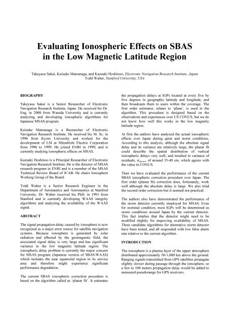
<str<strong>on</strong>g>Evaluat<strong>in</strong>g</str<strong>on</strong>g> <str<strong>on</strong>g>I<strong>on</strong>ospheric</str<strong>on</strong>g> <str<strong>on</strong>g>Effects</str<strong>on</strong>g> <strong>on</strong> <strong>SBAS</strong><br />
<strong>in</strong> <strong>the</strong> <strong>Low</strong> <strong>Magnetic</strong> Latitude Regi<strong>on</strong><br />
Takeyasu Sakai, Keisuke Matsunaga, and Kazuaki Hosh<strong>in</strong>oo, Electr<strong>on</strong>ic Navigati<strong>on</strong> Research Institute, Japan<br />
Todd Walter, Stanford University, USA<br />
BIOGRAPHY<br />
Takeyasu Sakai is a Senior Researcher of Electr<strong>on</strong>ic<br />
Navigati<strong>on</strong> Research Institute, Japan. He received his Dr.<br />
Eng. <strong>in</strong> 2000 from Waseda University and is currently<br />
analyz<strong>in</strong>g and develop<strong>in</strong>g i<strong>on</strong>ospheric algorithms for<br />
Japanese MSAS program.<br />
Keisuke Matsunaga is a Researcher of Electr<strong>on</strong>ic<br />
Navigati<strong>on</strong> Research Institute. He received his M. Sc. <strong>in</strong><br />
1996 from Kyoto University and worked for <strong>the</strong><br />
development of LSI at Mitsubishi Electric Corporati<strong>on</strong><br />
from 1996 to 1999. He jo<strong>in</strong>ed <strong>ENRI</strong> <strong>in</strong> 1999, and is<br />
currently study<strong>in</strong>g i<strong>on</strong>ospheric effects <strong>on</strong> MSAS.<br />
Kazuaki Hosh<strong>in</strong>oo is a Pr<strong>in</strong>cipal Researcher of Electr<strong>on</strong>ic<br />
Navigati<strong>on</strong> Research Institute. He is <strong>the</strong> director of MSAS<br />
research program <strong>in</strong> <strong>ENRI</strong> and is a member of <strong>the</strong> MSAS<br />
Technical Review Board of JCAB. He chairs I<strong>on</strong>osphere<br />
Work<strong>in</strong>g Group of <strong>the</strong> Board.<br />
Todd Walter is a Senior Research Eng<strong>in</strong>eer <strong>in</strong> <strong>the</strong><br />
Department of Aer<strong>on</strong>autics and Astr<strong>on</strong>autics at Stanford<br />
University. Dr. Walter received his PhD. <strong>in</strong> 1993 from<br />
Stanford and is currently develop<strong>in</strong>g WAAS <strong>in</strong>tegrity<br />
algorithms and analyz<strong>in</strong>g <strong>the</strong> availability of <strong>the</strong> WAAS<br />
signal.<br />
ABSTRACT<br />
The signal propagati<strong>on</strong> delay caused by i<strong>on</strong>osphere is now<br />
recognized as a major error source for satellite navigati<strong>on</strong><br />
systems. Because i<strong>on</strong>osphere is generated by solar<br />
radiati<strong>on</strong> and affected by <strong>the</strong> geomagnetic field, <strong>the</strong><br />
associated signal delay is very large and has significant<br />
variance <strong>in</strong> <strong>the</strong> low magnetic latitude regi<strong>on</strong>. The<br />
i<strong>on</strong>ospheric delay problem is currently <strong>the</strong> major c<strong>on</strong>cern<br />
for MSAS program (Japanese versi<strong>on</strong> of <strong>SBAS</strong>/WAAS)<br />
which <strong>in</strong>cludes <strong>the</strong> near equatorial regi<strong>on</strong> <strong>in</strong> its service<br />
area and <strong>the</strong>refore might experience significant<br />
performance degradati<strong>on</strong>.<br />
The current <strong>SBAS</strong> i<strong>on</strong>ospheric correcti<strong>on</strong> procedure is<br />
based <strong>on</strong> <strong>the</strong> algorithm called as ‘planar fit’. It estimates<br />
<strong>the</strong> propagati<strong>on</strong> delays at IGPs located at every five by<br />
five degrees <strong>in</strong> geographic latitude and l<strong>on</strong>gitude, and<br />
<strong>the</strong>n broadcasts <strong>the</strong>m to users with<strong>in</strong> <strong>the</strong> coverage. The<br />
first order estimator, relates to ‘plane’, is used <strong>in</strong> <strong>the</strong><br />
algorithm. This procedure is designed based <strong>on</strong> <strong>the</strong><br />
observati<strong>on</strong>s and experiences over US CONUS, but we do<br />
not know how well this works <strong>in</strong> <strong>the</strong> low magnetic<br />
latitude regi<strong>on</strong>.<br />
At first <strong>the</strong> authors have analyzed <strong>the</strong> actual i<strong>on</strong>ospheric<br />
effects over Japan dur<strong>in</strong>g quiet and storm c<strong>on</strong>diti<strong>on</strong>s.<br />
Accord<strong>in</strong>g to this analysis, although <strong>the</strong> absolute signal<br />
delay and its variance are relatively large, <strong>the</strong> planar fit<br />
could describe <strong>the</strong> spatial distributi<strong>on</strong> of vertical<br />
i<strong>on</strong>ospheric delays very well, and resulted <strong>in</strong> variance of<br />
residuals, σ decorr , of around 35-40 cm, which agrees with<br />
<strong>the</strong> value <strong>in</strong> CONUS.<br />
Then we have evaluated <strong>the</strong> performance of <strong>the</strong> current<br />
<strong>SBAS</strong> i<strong>on</strong>ospheric correcti<strong>on</strong> procedure over Japan. The<br />
first order (planar fit) correcti<strong>on</strong> does, fortunately, work<br />
well although <strong>the</strong> absolute delay is large. We also tried<br />
<strong>the</strong> sec<strong>on</strong>d order correcti<strong>on</strong> but it seemed not practical.<br />
The authors also have dem<strong>on</strong>strated <strong>the</strong> performance of<br />
<strong>the</strong> storm detector currently employed for MSAS. Even<br />
for nom<strong>in</strong>al c<strong>on</strong>diti<strong>on</strong>, most IGPs will be determ<strong>in</strong>ed as<br />
storm c<strong>on</strong>diti<strong>on</strong>s around Japan by <strong>the</strong> current detector.<br />
This fact implies that <strong>the</strong> detector might need to be<br />
modified slightly for improv<strong>in</strong>g availability of MSAS.<br />
Three candidate algorithms for alternative storm detector<br />
have been tested, and all resp<strong>on</strong>ded with low false alarm<br />
rate relative to <strong>the</strong> current algorithm.<br />
INTRODUCTION<br />
The i<strong>on</strong>osphere is a plasma layer of <strong>the</strong> upper atmosphere<br />
distributed approximately 50-1,000 km above <strong>the</strong> ground.<br />
Rang<strong>in</strong>g signals transmitted from GPS satellites propagate<br />
slightly slower dur<strong>in</strong>g passage through <strong>the</strong> i<strong>on</strong>osphere, so<br />
a few to 100 meters propagati<strong>on</strong> delay would be added to<br />
measured pseudorange for GPS receivers.
<str<strong>on</strong>g>I<strong>on</strong>ospheric</str<strong>on</strong>g> delay is now recognized as a major error<br />
source for satellite navigati<strong>on</strong> systems. ICAO <strong>SBAS</strong><br />
(satellite-based augmentati<strong>on</strong> system), def<strong>in</strong>ed by SARPs<br />
(<strong>in</strong>ternati<strong>on</strong>al standards and recommended practices) [1]<br />
documents, has a capability to make a correcti<strong>on</strong> to<br />
i<strong>on</strong>ospheric delay effects. It would broadcast users <strong>the</strong><br />
vertical i<strong>on</strong>ospheric delay estimates <strong>in</strong> meters at <strong>the</strong> grid<br />
po<strong>in</strong>ts (IGP; i<strong>on</strong>ospheric grid po<strong>in</strong>t) def<strong>in</strong>ed at every five<br />
by five degrees <strong>in</strong> geographic latitude and l<strong>on</strong>gitude.<br />
The <strong>SBAS</strong> i<strong>on</strong>ospheric correcti<strong>on</strong> procedure was actually<br />
def<strong>in</strong>ed based <strong>on</strong> <strong>the</strong> observati<strong>on</strong> and knowledge <strong>on</strong> <strong>the</strong><br />
i<strong>on</strong>ospheric activities over <strong>the</strong> US CONUS. In fact <strong>the</strong><br />
i<strong>on</strong>osphere has <strong>the</strong> significant activities <strong>in</strong> <strong>the</strong> equatorial<br />
regi<strong>on</strong>s while CONUS located <strong>in</strong> <strong>the</strong> relatively high<br />
magnetic latitude regi<strong>on</strong>. The equatorial anomalies affect<br />
<strong>on</strong> <strong>the</strong> large-scale structure of electr<strong>on</strong> density of<br />
i<strong>on</strong>osphere which might be difficult to be corrected by<br />
<strong>SBAS</strong> i<strong>on</strong>ospheric correcti<strong>on</strong> messages [2]. Plasma<br />
bubble effects (also known as depleti<strong>on</strong>), usually occur<br />
also <strong>in</strong> <strong>the</strong> low latitude regi<strong>on</strong>, might cause significant<br />
sc<strong>in</strong>tillati<strong>on</strong> which disrupts GPS signals [3][4]. ICAO<br />
<strong>SBAS</strong> IWG (Interoperability Work<strong>in</strong>g Group) meet<strong>in</strong>g<br />
has po<strong>in</strong>ted out this problem and now has organized<br />
specialized <strong>SBAS</strong> I<strong>on</strong>o-meet<strong>in</strong>gs frequently.<br />
<strong>SBAS</strong> is <strong>the</strong> <strong>in</strong>ternati<strong>on</strong>al standard system for global and<br />
seamless satellite-based navigati<strong>on</strong>, so it would be used<br />
even <strong>in</strong> <strong>the</strong> equatorial or low latitude regi<strong>on</strong>s. <strong>SBAS</strong><br />
providers need to <strong>in</strong>vestigate i<strong>on</strong>ospheric effects around<br />
<strong>the</strong> magnetic equator and <strong>the</strong> low magnetic latitude<br />
regi<strong>on</strong>s <strong>in</strong> terms of <strong>SBAS</strong> i<strong>on</strong>ospheric error correcti<strong>on</strong>.<br />
Japan is develop<strong>in</strong>g its own <strong>SBAS</strong> system, MSAS<br />
(MTSAT-based satellite augmentati<strong>on</strong> system; Japanese<br />
versi<strong>on</strong> of <strong>SBAS</strong>/WAAS) [5]. MSAS will cover a wide<br />
range of latitude (25N to 45N <strong>in</strong> geographic latitude; 15N<br />
to 35N <strong>in</strong> magnetic latitude) and <strong>the</strong> lowest magnetic<br />
latitude <strong>in</strong> <strong>the</strong> coverage is below 15 degrees magnetic<br />
north, which is close to <strong>the</strong> equatorial regi<strong>on</strong>.<br />
<str<strong>on</strong>g>I<strong>on</strong>ospheric</str<strong>on</strong>g> delay problem is currently <strong>the</strong> largest c<strong>on</strong>cern<br />
for MSAS program. Early this year <strong>the</strong> MSAS Technical<br />
Review Board of JCAB (Japan Civil Aviati<strong>on</strong> Bureau)<br />
established an I<strong>on</strong>osphere Work<strong>in</strong>g Group for this<br />
problem. Support<strong>in</strong>g such activities, <strong>the</strong> authors are<br />
<strong>in</strong>vestigat<strong>in</strong>g <strong>the</strong> i<strong>on</strong>ospheric effects over Japan to predict<br />
and improve <strong>the</strong> actual performance of MSAS <strong>on</strong> <strong>the</strong><br />
i<strong>on</strong>osphere.<br />
In this paper <strong>the</strong> authors will describe <strong>the</strong> performance of<br />
<strong>the</strong> current planar fit algorithm <strong>in</strong> <strong>the</strong> low magnetic<br />
latitude regi<strong>on</strong> with <strong>the</strong> m<strong>on</strong>itor site c<strong>on</strong>figurati<strong>on</strong> for<br />
MSAS. The sec<strong>on</strong>d order quadratic fit will also be tested<br />
as well as <strong>the</strong> first order planar fit. The activities of<br />
i<strong>on</strong>osphere over Japan will be characterized as some<br />
system parameters. The height of <strong>the</strong> actual i<strong>on</strong>osphere,<br />
which <strong>the</strong> current <strong>SBAS</strong> assumes as 350 km, is evaluated<br />
<str<strong>on</strong>g>I<strong>on</strong>ospheric</str<strong>on</strong>g><br />
delay<br />
IGP<br />
Rmax<br />
through <strong>the</strong> performance of planar fit. F<strong>in</strong>ally, <strong>the</strong><br />
performance of storm detector will be characterized and<br />
some alternatives are proposed.<br />
<strong>SBAS</strong> IONOSPHERIC CORRECTION<br />
IPPs used for planar fit<br />
IPPs not used<br />
2-nd order fit<br />
(6 parameters)<br />
1-st order fit<br />
(3 parameters)<br />
0-th order fit<br />
(1 parameter)<br />
Estimated delay at IGP<br />
Figure 1. Planar fit algorithm for <strong>SBAS</strong> i<strong>on</strong>ospheric<br />
delay estimati<strong>on</strong>. The current algorithm is <strong>the</strong> first<br />
order planar fit.<br />
<strong>SBAS</strong> i<strong>on</strong>ospheric correcti<strong>on</strong> procedure def<strong>in</strong>ed <strong>in</strong> SARPs<br />
[1] would be applied to remove i<strong>on</strong>ospheric delay effect<br />
and provide precise positi<strong>on</strong> to users. <strong>SBAS</strong> MCS would<br />
estimate signal propagati<strong>on</strong> delay at IGPs located every<br />
five by five degrees of geographic latitude and l<strong>on</strong>gitude<br />
with<strong>in</strong> <strong>the</strong> coverage regi<strong>on</strong>, and <strong>the</strong>n broadcast via <strong>the</strong><br />
<strong>SBAS</strong> geostati<strong>on</strong>ary satellite(s). User receivers apply <strong>the</strong><br />
broadcast correcti<strong>on</strong>s from <strong>the</strong> IGPs us<strong>in</strong>g bi-l<strong>in</strong>ear<br />
<strong>in</strong>terpolati<strong>on</strong>, <strong>in</strong> l<strong>in</strong>e with SARPs, or MOPS [6] def<strong>in</strong>ed<br />
for US WAAS.<br />
The broadcast format for propagati<strong>on</strong> delay <strong>in</strong>formati<strong>on</strong><br />
(MT18 and MT26) and <strong>the</strong> correcti<strong>on</strong> algorithm <strong>in</strong> user<br />
receivers are well-def<strong>in</strong>ed by SARPs while how MCS<br />
estimates <strong>the</strong> propagati<strong>on</strong> delay is open for service<br />
providers. Currently it seems that service providers tend<br />
to employ c<strong>on</strong>servative procedures and parameters for<br />
i<strong>on</strong>ospheric correcti<strong>on</strong>s because <strong>the</strong>y must ensure<br />
<strong>in</strong>tegrity requirements.<br />
The current estimator of i<strong>on</strong>ospheric propagati<strong>on</strong> delay<br />
for WAAS and MSAS is known as ‘planar fit’ [7]. For an<br />
IGP, <strong>the</strong> MCS generates a plane which fits <strong>the</strong> observed<br />
vertical i<strong>on</strong>ospheric delays at <strong>the</strong> surround<strong>in</strong>g IPPs at <strong>the</strong><br />
same <strong>in</strong>stant. Then <strong>the</strong> value at <strong>the</strong> orig<strong>in</strong> is <strong>the</strong> delay<br />
estimate for <strong>the</strong> IGP (See Figure 1). Each IPP should be<br />
with<strong>in</strong> R max = 2,100 km radius from <strong>the</strong> IGP. If <strong>the</strong><br />
number of collected IPPs is less than N m<strong>in</strong> = 10, <strong>the</strong><br />
planar fit is no l<strong>on</strong>ger valid and <strong>the</strong> IGP is set to ‘not<br />
m<strong>on</strong>itored’. Note that <strong>the</strong> zeroth and sec<strong>on</strong>d order fit are
also drawn <strong>in</strong> Figure 1 although <strong>the</strong> current <strong>SBAS</strong><br />
employs <strong>on</strong>ly <strong>the</strong> first order plane.<br />
The i<strong>on</strong>ospheric delay around <strong>the</strong> IGP (latitude φ IGP and<br />
l<strong>on</strong>gitude λ IGP ) is estimated by<br />
60<br />
MSAS M<strong>on</strong>itors<br />
User Stati<strong>on</strong>s<br />
IGS (Ref. <strong>on</strong>ly)<br />
MSAS service area<br />
45<br />
( λ,<br />
∆φ<br />
) = aˆ<br />
+ a ˆ ⋅ ∆λ<br />
+ a ⋅ ∆φ<br />
Iˆ<br />
v,IGP , (1)<br />
∆ 0 1<br />
ˆ2<br />
where ∆ λ = λ − λIGP<br />
, ∆φ<br />
= φ − φIGP<br />
. Fitt<strong>in</strong>g parameters<br />
could be solved by<br />
Latitude, N<br />
45<br />
30<br />
T<br />
T −1<br />
[ a0 a ˆ 1 aˆ<br />
2 ] = ( G ⋅W<br />
⋅ G ) ⋅ G ⋅W<br />
⋅ I v, IPP<br />
ˆ , (2)<br />
30<br />
where <strong>the</strong> observati<strong>on</strong> matrix is<br />
⎡1<br />
⎢<br />
⎢<br />
1<br />
G =<br />
⎢M<br />
⎢<br />
⎣1<br />
∆λ<br />
∆λ<br />
∆λ<br />
IPP1<br />
IPP2<br />
M<br />
IPPn<br />
∆φ<br />
∆φ<br />
∆φ<br />
IPP1<br />
IPP2<br />
M<br />
IPPn<br />
⎤<br />
⎥<br />
⎥ , (3)<br />
⎥<br />
⎥<br />
⎦<br />
and observed vertical i<strong>on</strong>ospheric delay values at IPPs are<br />
given by<br />
I v,IPP<br />
⎡I<br />
⎢<br />
⎢<br />
I<br />
=<br />
⎢<br />
⎢<br />
⎢⎣<br />
I<br />
v,<br />
IPP1<br />
v,<br />
IPP2<br />
M<br />
v,<br />
IPPn<br />
⎤<br />
⎥<br />
⎥ . (4)<br />
⎥<br />
⎥<br />
⎥⎦<br />
Vertical i<strong>on</strong>ospheric delay at <strong>the</strong> IGP is equal to â 0 , and<br />
Eqn. (1) can be applied at any locati<strong>on</strong> around <strong>the</strong> IGP.<br />
Additi<strong>on</strong>ally, <strong>the</strong> MCS must determ<strong>in</strong>e <strong>the</strong> variance of <strong>the</strong><br />
estimate as well as <strong>the</strong> absolute delay, to broadcast GIVE<br />
values. User receivers use GIVE (grid i<strong>on</strong>osphere vertical<br />
error) values to compute <strong>the</strong> c<strong>on</strong>fidence bound of positi<strong>on</strong><br />
estimate for provid<strong>in</strong>g <strong>in</strong>tegrity. Once <strong>the</strong> plane is<br />
generated and vertical delay at <strong>the</strong> orig<strong>in</strong> is estimated,<br />
formal error estimate can be computed <strong>in</strong> terms of 1-<br />
sigma expectati<strong>on</strong>.<br />
T<br />
( G ⋅W<br />
⋅G<br />
)<br />
1<br />
ˆ ⎡<br />
−<br />
σ<br />
⎤<br />
2ˆ =<br />
. (5)<br />
I v,<br />
IGP ⎢⎣<br />
⎥⎦<br />
Propagati<strong>on</strong> delays at IPPs are obta<strong>in</strong>ed from L1/L2 dual<br />
frequency measurements at M<strong>on</strong>itor Stati<strong>on</strong>s with slantto-vertical<br />
c<strong>on</strong>versi<strong>on</strong> below, assum<strong>in</strong>g th<strong>in</strong> shell<br />
i<strong>on</strong>osphere at <strong>the</strong> height of Hi<strong>on</strong>o<br />
= 350 km above <strong>the</strong><br />
ground,<br />
1,1<br />
MLAT<br />
15<br />
120 135 150 165<br />
L<strong>on</strong>gitude, E<br />
Figure 2. Distributi<strong>on</strong> of observati<strong>on</strong> sites for <strong>the</strong><br />
dataset.<br />
I<br />
v<br />
=<br />
⎛ RE<br />
⎞<br />
1 −<br />
⎜ cosE<br />
⋅ Islant<br />
RE<br />
H<br />
⎟ , (6)<br />
⎝ + i<strong>on</strong>o ⎠<br />
where R E is radius of <strong>the</strong> earth; and E is satellite<br />
elevati<strong>on</strong> angle above <strong>the</strong> horiz<strong>on</strong>.<br />
DATASET<br />
For <strong>in</strong>vestigat<strong>in</strong>g i<strong>on</strong>ospheric effects <strong>on</strong> <strong>SBAS</strong>, at first we<br />
need appropriate datasets of i<strong>on</strong>ospheric propagati<strong>on</strong><br />
delay observati<strong>on</strong>s dur<strong>in</strong>g quiet and stormy geomagnetic<br />
c<strong>on</strong>diti<strong>on</strong>s. The datasets should be taken at <strong>the</strong> m<strong>on</strong>itor<br />
stati<strong>on</strong>s for <strong>the</strong> <strong>SBAS</strong>, but it is not limited to just <strong>the</strong>se,<br />
because observati<strong>on</strong>s obta<strong>in</strong>ed at extra stati<strong>on</strong>s are useful<br />
for <strong>in</strong>vestigat<strong>in</strong>g some problems due to sampl<strong>in</strong>g density<br />
described later.<br />
<str<strong>on</strong>g>I<strong>on</strong>ospheric</str<strong>on</strong>g> delay may be measured by different ways:<br />
L1/L2 code divergence provides i<strong>on</strong>ospheric delay<br />
measurements but are noisy due to multipath <strong>on</strong> both<br />
frequencies; L1 code-carrier divergence has good<br />
availability of measurements due to lack of necessity for<br />
<strong>the</strong> relatively weak L2 signal, but is still disturbed by<br />
noise; here we have c<strong>on</strong>structed <strong>the</strong> dataset us<strong>in</strong>g L1/L2<br />
carrier divergence which provides very smooth noiseless<br />
measurements. Nuisance <strong>in</strong>teger cycle ambiguities<br />
<strong>in</strong>volved <strong>in</strong> carrier phase measurements are removed by<br />
averag<strong>in</strong>g to code measurements [8]. Based <strong>on</strong> temporal<br />
c<strong>on</strong>t<strong>in</strong>uity of i<strong>on</strong>ospheric delay measurements, cycle slips<br />
are detected and removed.<br />
2
Figure 3. 2-D histogram represent<strong>in</strong>g <strong>the</strong> distributi<strong>on</strong><br />
of differential vertical delays without planar fitt<strong>in</strong>g<br />
versus IPP separati<strong>on</strong>. No storm detector.<br />
Figure 5. 2-D histogram represent<strong>in</strong>g <strong>the</strong> distributi<strong>on</strong><br />
of differential vertical delays after planar fitt<strong>in</strong>g<br />
versus IPP separati<strong>on</strong>. No storm detector.<br />
elevati<strong>on</strong> mask at 5 degrees, we have <strong>the</strong> desired dataset<br />
for <strong>in</strong>vestigati<strong>on</strong>.<br />
Figure 4. 2-D histogram represent<strong>in</strong>g <strong>the</strong> distributi<strong>on</strong><br />
of differential vertical delays without planar fitt<strong>in</strong>g<br />
versus IPP separati<strong>on</strong>. This histogram represents<br />
stormy c<strong>on</strong>diti<strong>on</strong> of i<strong>on</strong>osphere. No storm detector.<br />
When us<strong>in</strong>g dual frequency measurements, an important<br />
error source for datasets is <strong>in</strong>strument bias error between<br />
two frequencies <strong>in</strong>herent to each <strong>in</strong>dividual satellite and<br />
receiver, sometimes called <strong>in</strong>ter-frequency bias (IFB)<br />
[9][10]. A Kalman filter has been applied to estimate such<br />
<strong>in</strong>strument biases [8][11] with an i<strong>on</strong>ospheric model of<br />
third-order spherical harm<strong>on</strong>ics basis functi<strong>on</strong>s placed <strong>on</strong><br />
three layers at 250, 350, and 450 km above <strong>the</strong> ground (a<br />
total of 48 unknowns for i<strong>on</strong>ospheric model; plus 27-28<br />
unknowns for satellite IFBs and 28 unknowns for receiver<br />
IFBs) <strong>in</strong> <strong>the</strong> solar-magnetic coord<strong>in</strong>ates. Elevati<strong>on</strong> mask<br />
angle was set to 15 degrees; optimal sett<strong>in</strong>g for estimat<strong>in</strong>g<br />
<strong>in</strong>strument biases correctly. We c<strong>on</strong>firmed that estimated<br />
biases repeated <strong>the</strong> same values for every analysis even<br />
for different periods. F<strong>in</strong>ally, after remov<strong>in</strong>g <strong>the</strong> estimates<br />
of <strong>in</strong>strument biases for each satellite and receiver from<br />
<strong>the</strong> orig<strong>in</strong>al L1/L2 carrier divergence observati<strong>on</strong> with<br />
Raw observati<strong>on</strong> data was provided by <strong>the</strong> GEONET GPS<br />
observati<strong>on</strong> network operated by Japan's Geographical<br />
Survey Institute s<strong>in</strong>ce 1994. For <strong>the</strong>se five or more years<br />
it has nearly 1,000 stati<strong>on</strong>s separated every 20-30 km <strong>in</strong><br />
Japan, and fur<strong>the</strong>rmore it was expanded to have 1,200<br />
stati<strong>on</strong>s <strong>in</strong> this year. All stati<strong>on</strong>s <strong>in</strong> <strong>the</strong> network have dualfrequency<br />
survey-grade GPS receivers and provide <strong>the</strong>ir<br />
measurements at every 30 sec<strong>on</strong>ds <strong>in</strong> <strong>the</strong> RINEX format.<br />
We chose 28 stati<strong>on</strong>s from this network as shown <strong>in</strong><br />
Figure 2 and created <strong>the</strong> i<strong>on</strong>ospheric delay datasets<br />
without cycle slips or IFBs. 6 IGS stati<strong>on</strong>s were also used<br />
to improve stability of IFB estimati<strong>on</strong> processes.<br />
Our purpose is survey<strong>in</strong>g how well <strong>the</strong> <strong>SBAS</strong> i<strong>on</strong>ospheric<br />
correcti<strong>on</strong> procedure works <strong>in</strong> <strong>the</strong> low magnetic latitude<br />
regi<strong>on</strong>, <strong>in</strong> particular around Japan. At first we were<br />
<strong>in</strong>terested <strong>in</strong> <strong>the</strong> observed uncerta<strong>in</strong>ty <strong>in</strong>volved <strong>in</strong><br />
i<strong>on</strong>ospheric delays. For a typical quiet day, as <strong>in</strong> Figure 3,<br />
<strong>the</strong> difference of vertical i<strong>on</strong>ospheric delays observed at<br />
two IPPs reaches 2-3 meters between zero-distance IPPs,<br />
and up to 8 meters between IPPs separated 2,000 km or<br />
more. For storm days, Figure 4, it sometimes reaches 7-8<br />
meters for zero-distance, and 15 meters or more even at<br />
1,000 km separati<strong>on</strong>. The problem is now how well <strong>the</strong><br />
<strong>SBAS</strong> i<strong>on</strong>ospheric correcti<strong>on</strong> procedure could correct<br />
such significant uncerta<strong>in</strong>ty of i<strong>on</strong>ospheric delays.<br />
CHARACTERIZATION<br />
The i<strong>on</strong>ospheric activity <strong>in</strong> <strong>the</strong> low magnetic latitude<br />
regi<strong>on</strong>, i.e., over Japan, should be characterized for<br />
analysis and predicti<strong>on</strong> of <strong>the</strong> actual system. Some<br />
parameters are used for such characterizati<strong>on</strong>; σ decorr is
Estimated Sigma, m<br />
Estimated Sigma, m<br />
3<br />
2<br />
1<br />
0<br />
3<br />
2<br />
1<br />
68.3%<br />
95.5%<br />
99.7%<br />
68.3%<br />
95.5%<br />
99.7%<br />
No Fitt<strong>in</strong>g<br />
Planar Fitt<strong>in</strong>g<br />
0<br />
0 1000 2000 3000<br />
IPP Distance, km<br />
Figure 6. Variance of differential vertical delays,<br />
computed based <strong>on</strong> 1-, 2-, and 3- sigma, versus IPP<br />
separati<strong>on</strong> for a quiet i<strong>on</strong>ospheric c<strong>on</strong>diti<strong>on</strong>. After<br />
planar fit removal, distributi<strong>on</strong> of <strong>the</strong> residuals<br />
becomes away from <strong>the</strong> normal distributi<strong>on</strong>.<br />
<strong>on</strong>e of <strong>the</strong>m which relates to variance of differential<br />
i<strong>on</strong>ospheric delay after removal of a planar fit estimate.<br />
Figure 5 is a 2-dimensi<strong>on</strong>al histogram which represents<br />
<strong>the</strong> distributi<strong>on</strong> of differential i<strong>on</strong>ospheric delays after<br />
planar fit corresp<strong>on</strong>d<strong>in</strong>g to IPP separati<strong>on</strong> for quiet<br />
c<strong>on</strong>diti<strong>on</strong> of i<strong>on</strong>osphere (Compare with Figure 3). The<br />
differential delays are spatially decorrelated so <strong>the</strong><br />
distributi<strong>on</strong> becomes compact, but tails of <strong>the</strong> distributi<strong>on</strong><br />
seems to spread a pretty wide. Note that a total of 31<br />
stati<strong>on</strong>s (<strong>in</strong>clud<strong>in</strong>g all stati<strong>on</strong>s <strong>in</strong> Figure 2) are used to<br />
create this plot because characterizati<strong>on</strong> of i<strong>on</strong>osphere<br />
should be d<strong>on</strong>e with as many stati<strong>on</strong>s as possible<br />
regardless of <strong>the</strong> c<strong>on</strong>figurati<strong>on</strong> of MSAS m<strong>on</strong>itor stati<strong>on</strong>s.<br />
Variance of differential i<strong>on</strong>ospheric delays can be<br />
characterized based <strong>on</strong> 1-, 2-, and 3- sigma values. Figure<br />
6 shows estimated sigma values with and without planar<br />
fit removal, versus IPP separati<strong>on</strong>. The bottom plot is<br />
with planar fit removal, actually corresp<strong>on</strong>ds to <strong>the</strong><br />
parameter σ decorr . Note that while <strong>the</strong> distributi<strong>on</strong> of<br />
M<strong>on</strong>itor Stati<strong>on</strong>s (6)<br />
Provides IPPs<br />
Collects IPPs<br />
Surround<strong>in</strong>g <strong>the</strong> IGP<br />
Planar Fit<br />
Centered at <strong>the</strong> IGP<br />
Estimates Delay<br />
at <strong>the</strong> IGP<br />
<str<strong>on</strong>g>I<strong>on</strong>ospheric</str<strong>on</strong>g> Delay Datasets<br />
IGP Locati<strong>on</strong><br />
Estimated<br />
Delay<br />
differential i<strong>on</strong>ospheric delays is almost normal without<br />
planar fit, after planar fit removal <strong>the</strong> distributi<strong>on</strong> moves<br />
away from <strong>the</strong> normal distributi<strong>on</strong> with hav<strong>in</strong>g tails<br />
spread<strong>in</strong>g wide. Accord<strong>in</strong>g to 1-sigma plot <strong>in</strong> <strong>the</strong> bottom<br />
of Figure 6, σ decorr value could be around 35-40 cm, which<br />
agrees with <strong>the</strong> value <strong>in</strong> CONUS, 35 cm for WAAS [12].<br />
In c<strong>on</strong>trast with case of WAAS, however, three curves <strong>in</strong><br />
<strong>the</strong> bottom plot of Figure 6 have clear correlati<strong>on</strong> with<br />
IPP separati<strong>on</strong>.<br />
PERFORMANCE OF PLANAR FIT<br />
User Stati<strong>on</strong>s (16)<br />
Provides IGPs<br />
Fetch IGP <strong>on</strong>e-by-<strong>on</strong>e<br />
Compare<br />
Residual Error<br />
Figure 7. Evaluati<strong>on</strong> Process. Orig<strong>in</strong>al dataset is<br />
divided <strong>in</strong>to two parts. Partial set of M<strong>on</strong>itor Stati<strong>on</strong>s<br />
is used for estimat<strong>in</strong>g i<strong>on</strong>ospheric delay by planar fit<br />
centered at <strong>the</strong> IGP. Sec<strong>on</strong>d set of User Stati<strong>on</strong>s<br />
provides IGP observati<strong>on</strong>s to be compared with<br />
resulted estimati<strong>on</strong>.<br />
For evaluat<strong>in</strong>g <strong>SBAS</strong> i<strong>on</strong>ospheric correcti<strong>on</strong> capability,<br />
we applied <strong>the</strong> planar fit algorithm to <strong>the</strong> observed<br />
i<strong>on</strong>ospheric delay datasets described above. At first, <strong>the</strong><br />
orig<strong>in</strong>al dataset is divided <strong>in</strong>to two parts; sets of M<strong>on</strong>itor<br />
Stati<strong>on</strong>s and User Stati<strong>on</strong>s (Figure 7).<br />
MSAS has 6 m<strong>on</strong>itor stati<strong>on</strong>s <strong>in</strong> Japan, so we applied<br />
planar fit algorithm based <strong>on</strong> IPPs collected by 6<br />
GEONET stati<strong>on</strong>s co-located by MSAS m<strong>on</strong>itor stati<strong>on</strong>s<br />
(Red stati<strong>on</strong>s <strong>in</strong> Figure 2). These stati<strong>on</strong>s should be called<br />
as M<strong>on</strong>itor Stati<strong>on</strong>s which provide IPP measurements to<br />
be used for analysis.<br />
In order to evaluate <strong>the</strong> performance of <strong>the</strong> algorithms at<br />
<strong>the</strong> IGP, we have used 16 stati<strong>on</strong>s (Green stati<strong>on</strong>s <strong>in</strong><br />
Figure 2) o<strong>the</strong>r than MSAS 6 m<strong>on</strong>itor stati<strong>on</strong>s. Because<br />
<strong>SBAS</strong> must bound user positi<strong>on</strong><strong>in</strong>g error at any<br />
(unknown) user locati<strong>on</strong>, we need to evaluate its<br />
performance us<strong>in</strong>g <strong>the</strong>se User Stati<strong>on</strong>s which provide IGP<br />
measurements, o<strong>the</strong>r than M<strong>on</strong>itor Stati<strong>on</strong>s above.
Figure 8. Histogram plots of planar fit residuals for<br />
quiet c<strong>on</strong>diti<strong>on</strong>.<br />
Figure 10. Histogram plots of planar fit residuals for<br />
storm c<strong>on</strong>diti<strong>on</strong>. Compare with Figure 5.<br />
Figure 9. (Top) Histogram plots of quadratic fit<br />
(sec<strong>on</strong>d order) residuals for quiet c<strong>on</strong>diti<strong>on</strong>. (Bottom)<br />
Applied 4-of-4 geometry check and removed IGPs<br />
with bad geometry. IGP availability decreased to<br />
58.3%.<br />
In this analysis, each residual error was obta<strong>in</strong>ed as <strong>the</strong><br />
difference between IGP vertical delay observed from User<br />
Stati<strong>on</strong>s and <strong>the</strong> corresp<strong>on</strong>d<strong>in</strong>g vertical delay estimati<strong>on</strong><br />
computed by IPPs surround<strong>in</strong>g <strong>the</strong> IGP observed from<br />
Figure 11. (Top) Histogram plots of quadratic fit<br />
(sec<strong>on</strong>d order) residuals for storm c<strong>on</strong>diti<strong>on</strong>.<br />
(Bottom) Applied 4-of-4 geometry check and removed<br />
IGPs with bad geometry. IGP availability decreased<br />
to 55.9%.<br />
M<strong>on</strong>itor Stati<strong>on</strong>s. Vertical delays observed from M<strong>on</strong>itor<br />
Stati<strong>on</strong>s have not been used as IGPs.
Planar and Quadratic Fit: Quiet and Storm<br />
Figure 8 shows a histogram plot of residual errors after<br />
planar fit removal for quiet i<strong>on</strong>ospheric c<strong>on</strong>diti<strong>on</strong>. RMS<br />
residual was 0.564 meter and residual errors were<br />
bounded with<strong>in</strong> 3.56 meters although no storm detectors<br />
applied.<br />
One possible way to improve correcti<strong>on</strong> performance may<br />
be apply<strong>in</strong>g quadratic fit (sec<strong>on</strong>d order fitt<strong>in</strong>g). Vertical<br />
i<strong>on</strong>ospheric delay should be modeled below <strong>in</strong>stead of<br />
Eqn. (1),<br />
ˆ<br />
( ∆λ,<br />
∆φ<br />
)<br />
ˆ<br />
I v,IGP = a0<br />
+ a1<br />
⋅ ∆λ<br />
+ a2<br />
⋅ ∆φ<br />
, (7)<br />
+ aˆ<br />
⋅ ∆λ<br />
⋅ ∆φ<br />
+ aˆ<br />
⋅<br />
3<br />
ˆ<br />
ˆ<br />
4<br />
2<br />
( ∆λ<br />
) + aˆ<br />
⋅ ( ∆φ<br />
) 2<br />
5<br />
Figure 12. The distributi<strong>on</strong> of User Stati<strong>on</strong>s for<br />
c<strong>on</strong>siderati<strong>on</strong> of geometry of m<strong>on</strong>itor stati<strong>on</strong>s; (Left)<br />
User Stati<strong>on</strong>s <strong>in</strong>side <strong>the</strong> network of M<strong>on</strong>itor Stati<strong>on</strong>s;<br />
(Right) User Stati<strong>on</strong>s outside <strong>the</strong> network. Red circles<br />
represent <strong>the</strong> network of MSAS M<strong>on</strong>itor Stati<strong>on</strong>s.<br />
where 6 fitt<strong>in</strong>g parameters can be solved by <strong>the</strong> similar<br />
way to Eqn. (2).<br />
Figure 9 gives <strong>the</strong> sample results of quadratic fit for quiet<br />
i<strong>on</strong>ospheric c<strong>on</strong>diti<strong>on</strong>. Unfortunately RMS residual was<br />
1.043 meters so not improved aga<strong>in</strong>st planar fit , and more<br />
importantly, large correcti<strong>on</strong> errors sometimes occur. This<br />
is because <strong>in</strong>creas<strong>in</strong>g <strong>the</strong> number of fit parameters causes<br />
a reducti<strong>on</strong> of <strong>the</strong> number of degrees-of-freedom and <strong>the</strong><br />
geometries of <strong>the</strong> IPP distributi<strong>on</strong> was not good enough to<br />
perform a quadratic fit.<br />
To c<strong>on</strong>firm this, Figure 9 (b) shows quadratic fit results<br />
<strong>on</strong>ly for IGPs which have good geometry. A 4-of-4 check<br />
was applied here; <strong>the</strong> IGP must have at least <strong>on</strong>e IPP <strong>in</strong><br />
each of its 4 quadrants. With this geometry check<strong>in</strong>g,<br />
RMS residual was 0.520 meters and <strong>the</strong> maximum<br />
residual was improved to 2.94 meters. But <strong>the</strong> number of<br />
evaluated IGPs was 58.3% of <strong>the</strong> case without geometry<br />
check; this 4-of-4 geometry check lowered <strong>the</strong> availability<br />
of IGP. The quadratic fit essentially has better correcti<strong>on</strong><br />
capability, but it would provide relatively low number of<br />
available IGPs.<br />
Now we are go<strong>in</strong>g <strong>on</strong> to <strong>the</strong> storm c<strong>on</strong>diti<strong>on</strong>. The planar<br />
fit is applied to <strong>the</strong> dataset taken dur<strong>in</strong>g storm i<strong>on</strong>ospheric<br />
c<strong>on</strong>diti<strong>on</strong>s, represented <strong>in</strong> Figure 4. The histogram plot of<br />
result<strong>in</strong>g residual error is illustrated <strong>in</strong> Figure 10. RMS<br />
residual error grew 0.759 meter and <strong>the</strong> maximum was<br />
12.02 meters. The asymmetric histogram <strong>in</strong>volves many<br />
positive large residuals; this means <strong>the</strong>re are large<br />
‘mounta<strong>in</strong>s’ to which planar fit cannot correct properly.<br />
A quadratic fit has <strong>the</strong> capability to correct such large<br />
‘mounta<strong>in</strong>s’ accord<strong>in</strong>g to Figure 11 (b) which has <strong>the</strong><br />
property of symmetry. However, <strong>the</strong> quadratic fit still<br />
requires some geometry check. The performances of<br />
planar and quadratic fit are summarized <strong>in</strong> Table 1.<br />
(a) Inside stati<strong>on</strong>s<br />
(b) Outside stati<strong>on</strong>s<br />
Figure 13. Histogram plots of planar fit residuals for<br />
storm c<strong>on</strong>diti<strong>on</strong>. (a) User stati<strong>on</strong>s are located <strong>in</strong>side<br />
<strong>the</strong> network of M<strong>on</strong>itor Stati<strong>on</strong>s; (b) User stati<strong>on</strong>s are<br />
outside <strong>the</strong> network.<br />
Geometry of M<strong>on</strong>itor Stati<strong>on</strong>s<br />
The residual errors of i<strong>on</strong>ospheric correcti<strong>on</strong> caused by<br />
<strong>the</strong> <strong>SBAS</strong> procedure can be decomposed as: (i) measure-
Table 1. Performance of Planar Fit<br />
C<strong>on</strong>diti<strong>on</strong><br />
User Stati<strong>on</strong><br />
Geometry Residuals, m<br />
Order<br />
Set<br />
Check RMS Max.<br />
1 No 0.564 3.56<br />
Quiet Whole 16<br />
2 No 1.04 22.5<br />
1 4-of-4 0.498 2.91<br />
2 4-of-4 0.520 2.94<br />
1 No 0.759 12.0<br />
Whole 16<br />
2 No 1.58 92.8<br />
1 4-of-4 0.551 5.68<br />
2 4-of-4 0.531 5.94<br />
1 No 0.635 8.30<br />
Storm Inside 7<br />
2 No 0.620 24.8<br />
1 4-of-4 0.525 5.68<br />
2 4-of-4 0.479 5.52<br />
1 No 0.787 12.0<br />
Outside 8<br />
2 No 1.67 77.9<br />
1 4-of-4 0.5678 7.65<br />
2 4-of-4 0.5683 8.70<br />
Evaluated<br />
IPPs<br />
67.6 %<br />
39.4 %<br />
68.1 %<br />
38.1 %<br />
53.1 %<br />
37.7 %<br />
52.0 %<br />
23.4 %<br />
Figure 14. The performance of planar fit with respect to shell height. Local time is UT+9h.
ment error at <strong>the</strong> m<strong>on</strong>itor stati<strong>on</strong>s (cycle slips, multipath,<br />
etc.); (ii) undersampl<strong>in</strong>g (MSAS has <strong>on</strong>ly 6 m<strong>on</strong>itor<br />
stati<strong>on</strong>s); (iii) th<strong>in</strong> shell assumpti<strong>on</strong>; (iv) i<strong>on</strong>ospheric<br />
height assumpti<strong>on</strong> (350 km for <strong>SBAS</strong>); (v) spatial<br />
resoluti<strong>on</strong> of correcti<strong>on</strong> <strong>in</strong>formati<strong>on</strong> (five by five<br />
degrees); (vi) broadcast<strong>in</strong>g <strong>in</strong>terval (maximum 5<br />
m<strong>in</strong>utes); (vii) quantizati<strong>on</strong> error (0.125 meter <strong>in</strong> MT26).<br />
We evaluated effects of (ii), (iii), and (iv) <strong>in</strong> Figures 8-11.<br />
Here <strong>the</strong> effect of (ii) undersampl<strong>in</strong>g problem has an<br />
emphasis.<br />
Aga<strong>in</strong>, Figure 13 relates to <strong>the</strong> performance of <strong>the</strong> first<br />
order planar fit for storm c<strong>on</strong>diti<strong>on</strong> of i<strong>on</strong>osphere.<br />
Histogram plot (a) shows resulted residual errors after<br />
planar fit at IGPs observed from 7 of 16 User Stati<strong>on</strong>s<br />
located <strong>in</strong>side <strong>the</strong> network of M<strong>on</strong>itor Stati<strong>on</strong>s. (b)<br />
displays evaluati<strong>on</strong> by <strong>the</strong> o<strong>the</strong>r 8 User Stati<strong>on</strong>s located<br />
outside <strong>the</strong> network. Both results are without any<br />
geometry check nor storm detectors. The distributi<strong>on</strong> of<br />
User Stati<strong>on</strong>s is illustrated <strong>in</strong> Figure 12.<br />
Figure 15. Performance of chi-square storm detector.<br />
Each IPP is determ<strong>in</strong>ed as storm c<strong>on</strong>diti<strong>on</strong> if <strong>the</strong><br />
corresp<strong>on</strong>d<strong>in</strong>g m<strong>on</strong>itor output is greater than 1.<br />
Detecti<strong>on</strong> Threshold<br />
The first order planar fit for <strong>in</strong>side stati<strong>on</strong>s resulted <strong>in</strong><br />
RMS residuals of 0.635 meter while 0.787 meter for<br />
outside stati<strong>on</strong>s. The maximum residuals were 8.30<br />
meters and 12.04 meters, respectively. Compar<strong>in</strong>g Figure<br />
13 (b) with Figure 10, <strong>the</strong>se Figures are almost identical,<br />
we can see that most of large residual errors are<br />
corresp<strong>on</strong>d<strong>in</strong>g to outside stati<strong>on</strong>s.<br />
Residual<br />
Error [m]<br />
(Unknown)<br />
Missed<br />
Detecti<strong>on</strong><br />
IGP<br />
Available<br />
IGP<br />
Unavailable<br />
(Storm)<br />
False<br />
Alarm<br />
Bound<strong>in</strong>g<br />
Requirement<br />
While <strong>the</strong> RMS of residual errors are almost identical for<br />
both sets of stati<strong>on</strong>s, <strong>the</strong> largest error were 5.68 meters for<br />
<strong>in</strong>side stati<strong>on</strong>s and 7.65 meters for outside stati<strong>on</strong>s.<br />
Shell Height C<strong>on</strong>siderati<strong>on</strong><br />
For <strong>the</strong> current <strong>SBAS</strong>, <strong>the</strong> i<strong>on</strong>osphere is assumed to be at<br />
a th<strong>in</strong> shell with <strong>the</strong> fixed height of 350 km. It is well<br />
known <strong>the</strong> actual i<strong>on</strong>osphere is not stati<strong>on</strong>ary and changes<br />
<strong>the</strong> height due to time of <strong>the</strong> day as well as seas<strong>on</strong> <strong>in</strong> <strong>the</strong><br />
year and solar activities.<br />
Figure 14 dem<strong>on</strong>strates <strong>the</strong> relati<strong>on</strong>ship between shell<br />
height assumpti<strong>on</strong> and <strong>the</strong> fitt<strong>in</strong>g performance. RMS<br />
residual error is <strong>the</strong> lowest when <strong>the</strong> shell height is set to<br />
500 km or more dur<strong>in</strong>g daytime (00-12h UT; 09-21h<br />
local). At local night, <strong>the</strong> height of i<strong>on</strong>osphere which<br />
provides <strong>the</strong> best performance decreased, and <strong>in</strong> <strong>the</strong> early<br />
morn<strong>in</strong>g (20-24h UT; 05-09 local) it was at 350 km.<br />
The difference <strong>in</strong> RMS for various shell height is,<br />
however, <strong>on</strong>ly 0.1 meter or less. In comparis<strong>on</strong> with <strong>the</strong><br />
complexity of mechanism for chang<strong>in</strong>g shell height <strong>in</strong> <strong>the</strong><br />
MCS and/or user receivers, this potential improvement of<br />
<strong>the</strong> i<strong>on</strong>ospheric model is relatively small.<br />
STORM DETECTOR<br />
Detector Output<br />
(Computable)<br />
Figure 16. Def<strong>in</strong>iti<strong>on</strong> of IGP status. Note that residual<br />
error is unknown for <strong>the</strong> actual system.<br />
In case of MSAS, <strong>on</strong>e reas<strong>on</strong> for relatively low<br />
availability for APV operati<strong>on</strong>s is that most IGPs will be<br />
set as be<strong>in</strong>g <strong>in</strong> <strong>the</strong> storm c<strong>on</strong>diti<strong>on</strong> for which users could<br />
not expect valid i<strong>on</strong>ospheric correcti<strong>on</strong>, even for nom<strong>in</strong>al<br />
c<strong>on</strong>diti<strong>on</strong>. It seemed that <strong>the</strong> chi-square storm detector<br />
currently built <strong>in</strong> MSAS MCS algorithm has worked <strong>in</strong><br />
very sensitive or c<strong>on</strong>servative manner.<br />
This fact motivated us to c<strong>on</strong>sider of detecti<strong>on</strong> algorithms<br />
o<strong>the</strong>r than <strong>on</strong>e based <strong>on</strong> chi-square test. If <strong>the</strong>re is an<br />
algorithm to detect storm c<strong>on</strong>diti<strong>on</strong> of i<strong>on</strong>osphere better<br />
than chi-square test, it could improve <strong>the</strong> availability for<br />
APV operati<strong>on</strong>s. First of all, chi-square statistics for storm<br />
c<strong>on</strong>diti<strong>on</strong> are shown <strong>in</strong> Figure 15. Ideally, residual errors<br />
should be small if <strong>the</strong> detector output is less than 1; <strong>on</strong> <strong>the</strong><br />
o<strong>the</strong>r hand, <strong>the</strong> detector must <strong>in</strong>dicate storm c<strong>on</strong>diti<strong>on</strong><br />
with <strong>the</strong> corresp<strong>on</strong>d<strong>in</strong>g output greater than 1 <strong>in</strong> case of<br />
large residual error. The current chi-square detector,<br />
unfortunately, implies no such feature.
Figure 16 def<strong>in</strong>es some status of IGP. Each IGP is<br />
determ<strong>in</strong>ed as available if <strong>the</strong> corresp<strong>on</strong>d<strong>in</strong>g detector<br />
output is less than a certa<strong>in</strong> threshold; <strong>in</strong> this case, missed<br />
detecti<strong>on</strong> would occur if actual residual error exceeds <strong>the</strong><br />
bound<strong>in</strong>g requirement. When detector output is greater<br />
than <strong>the</strong> threshold, <strong>the</strong> IGP is declared unavailable; if <strong>the</strong><br />
actual residual error is less than <strong>the</strong> requirement, this is a<br />
false alarm c<strong>on</strong>diti<strong>on</strong>. Note that missed detecti<strong>on</strong> and<br />
false alarm c<strong>on</strong>diti<strong>on</strong>s cannot be recognized for <strong>the</strong> actual<br />
system because <strong>the</strong> residual error at user locati<strong>on</strong> is<br />
unknown.<br />
We have tested three candidate algorithms for a storm<br />
detector:<br />
1. HDOP: computed based <strong>on</strong> geometry matrix relative<br />
to <strong>the</strong> IGP locati<strong>on</strong> (height could be set to zero) with<br />
IPPs used for planar fit.<br />
2. C<strong>on</strong>diti<strong>on</strong> Number: of <strong>the</strong> matrix used for planar fit.<br />
3. Distance to Centroid: The distance between IGP and<br />
<strong>the</strong> centroid of IPPs used for planar fit.<br />
IPPs could be weighted based <strong>on</strong> <strong>the</strong> corresp<strong>on</strong>d<strong>in</strong>g<br />
satellite elevati<strong>on</strong> angle.<br />
The performances of <strong>the</strong> candidate algorithms are<br />
evaluated with dataset dur<strong>in</strong>g October 2003 storm. Figure<br />
17 shows <strong>the</strong> relati<strong>on</strong>ship between residual errors and<br />
detector outputs. In comparis<strong>on</strong> with Figure 14, <strong>the</strong>se<br />
three algorithms give better performance but false alarm<br />
could not be lowered sufficiently.<br />
Given bound<strong>in</strong>g requirement and missed detecti<strong>on</strong> rate,<br />
<strong>on</strong>e can determ<strong>in</strong>e <strong>the</strong> detecti<strong>on</strong> threshold and <strong>the</strong>refore<br />
compute resulted false alarm rate. Table 2 summarizes <strong>the</strong><br />
performances of <strong>the</strong> candidate detectors <strong>in</strong> terms of false<br />
alarm rate with bound<strong>in</strong>g requirement of 5 meters. The<br />
current chi-square detector could give low false alarm rate<br />
but resulted a lot of missed detecti<strong>on</strong>. For missed<br />
detecti<strong>on</strong> rate 0.001, each algorithm reduces false alarm<br />
rate down to 40% while chi-square detector resulted false<br />
alarm of 90%.<br />
Figure 17. The performance plots for three candidate<br />
storm detector algorithms dur<strong>in</strong>g October 2003 storm.<br />
Compare with Figure 15 for <strong>the</strong> current chi-square<br />
detector.<br />
In our analysis, each candidate storm detector works<br />
based <strong>on</strong> <strong>the</strong> IPPs observed from 6 MSAS M<strong>on</strong>itor<br />
Stati<strong>on</strong>s. The output of detector is <strong>in</strong>dicated as horiz<strong>on</strong>tal<br />
axis. The residual errors are computed for IGPs observed<br />
from <strong>the</strong> o<strong>the</strong>r 16 User Stati<strong>on</strong>s, as same to case of<br />
Figures 7-11, and relate to <strong>the</strong> vertical axis of <strong>the</strong><br />
follow<strong>in</strong>g 2-D histogram plots.<br />
Note that <strong>the</strong> results shown here actually <strong>in</strong>volve<br />
undersampl<strong>in</strong>g effects. These candidate detectors measure<br />
Table 2. The performances of <strong>the</strong> candidate detectors<br />
(Bound<strong>in</strong>g Req. = 5 m).<br />
Algorithm<br />
Missed<br />
False<br />
Detecti<strong>on</strong><br />
Detecti<strong>on</strong><br />
Alarm<br />
Threshold<br />
Rate<br />
Rate<br />
Chi-square<br />
0.897 1.000 0.0149<br />
0.001 0.0352 0.920<br />
HDOP 0.001 0.793 0.401<br />
C<strong>on</strong>d. number 0.001 0.783 0.406<br />
Dist. to centroid 0.001 1.153 0.463
goodness (or badness) of ‘geometry’ of IPPs for planar fit<br />
distributed around <strong>the</strong> IGP. If <strong>the</strong>re is a large hole <strong>in</strong> <strong>the</strong><br />
distributi<strong>on</strong> of IPP, i.e., <strong>the</strong>re is a large area not sampled<br />
by <strong>the</strong> m<strong>on</strong>itor stati<strong>on</strong>s, <strong>the</strong>se detectors would determ<strong>in</strong>e<br />
<strong>the</strong> IGP is <strong>in</strong> ‘storm c<strong>on</strong>diti<strong>on</strong>’. Such c<strong>on</strong>diti<strong>on</strong>s do not<br />
always relate to <strong>the</strong> actual storm <strong>in</strong> fact, but <strong>the</strong><br />
corresp<strong>on</strong>d<strong>in</strong>g residual error can be expected to be large.<br />
This is a reas<strong>on</strong> we evaluated detectors at 16 User<br />
Stati<strong>on</strong>s o<strong>the</strong>r than MSAS M<strong>on</strong>itor Stati<strong>on</strong>s.<br />
Note also that <strong>the</strong> operati<strong>on</strong>al systems of WAAS and<br />
MSAS have a certa<strong>in</strong> mechanism to <strong>in</strong>volve such<br />
geometric metrics, as undersampled threat model,<br />
additi<strong>on</strong>al to <strong>the</strong> chi-square storm detector. Although <strong>the</strong><br />
chi-square detector passes over a lot of missed detecti<strong>on</strong><br />
c<strong>on</strong>diti<strong>on</strong>s, <strong>the</strong> model will bound <strong>the</strong> actual user rang<strong>in</strong>g<br />
error.<br />
CONCLUDING REMARKS<br />
The authors evaluated <strong>the</strong> current <strong>SBAS</strong> i<strong>on</strong>ospheric<br />
correcti<strong>on</strong> capability over Japan. The planar fit algorithm<br />
fortunately gave relatively satisfactory performance <strong>in</strong><br />
such low magnetic latitude regi<strong>on</strong> for LNAV/VNAV<br />
operati<strong>on</strong>s. The algorithm for storm detector might be<br />
modified so reduc<strong>in</strong>g false alarm rate for achiev<strong>in</strong>g <strong>the</strong><br />
capability of APV operati<strong>on</strong>s. We also evaluated<br />
undersampl<strong>in</strong>g effects by us<strong>in</strong>g additi<strong>on</strong>al pseudo-user<br />
stati<strong>on</strong>s which is essential for ensur<strong>in</strong>g <strong>in</strong>tegrity of <strong>SBAS</strong>.<br />
Fur<strong>the</strong>r <strong>in</strong>vestigati<strong>on</strong>s should <strong>in</strong>clude: evaluat<strong>in</strong>g o<strong>the</strong>r<br />
correcti<strong>on</strong> methods such as multi-layer i<strong>on</strong>ospheric model<br />
or Krig<strong>in</strong>g algorithm; sort<strong>in</strong>g out <strong>the</strong> relati<strong>on</strong>ship between<br />
storm detector and undersampl<strong>in</strong>g (essentially geometry)<br />
problem; c<strong>on</strong>sider<strong>in</strong>g temporal variati<strong>on</strong>s of i<strong>on</strong>osphere;<br />
and study<strong>in</strong>g sc<strong>in</strong>tillati<strong>on</strong> effects.<br />
[4] K. Matsunaga, K. Hosh<strong>in</strong>oo, and K. Igarashi,<br />
Observati<strong>on</strong>s of <str<strong>on</strong>g>I<strong>on</strong>ospheric</str<strong>on</strong>g> Sc<strong>in</strong>tillati<strong>on</strong> <strong>on</strong> GPS Signals<br />
<strong>in</strong> Japan, Navigati<strong>on</strong>, vol. 50, no. 1, pp. 1-7, Spr<strong>in</strong>g 2003.<br />
[5] J. Imamura, MSAS Program and Overview, Proc. 4th<br />
CGSIC IISC Asia Pacific Rim Meet<strong>in</strong>g, 2003 Jo<strong>in</strong>t<br />
Internati<strong>on</strong>al C<strong>on</strong>ference <strong>on</strong> GPS/GNSS, Tokyo, Nov.<br />
2003.<br />
[6] M<strong>in</strong>imum Operati<strong>on</strong>al Performance Standards for<br />
Global Positi<strong>on</strong><strong>in</strong>g System/Wide Area Augmentati<strong>on</strong><br />
System Airborne Equipment, DO-229C, RTCA, Nov.<br />
2001.<br />
[7] T. Walter, A. Hansen, J. Blanch, and P. Enge, Robust<br />
Detecti<strong>on</strong> of <str<strong>on</strong>g>I<strong>on</strong>ospheric</str<strong>on</strong>g> Irregularities, Proc. ION GPS,<br />
pp. 209-218, Salt Lake City, UT, Sept. 2000.<br />
[8] A. Hansen, Tomographic Estimati<strong>on</strong> of <strong>the</strong> I<strong>on</strong>osphere<br />
Us<strong>in</strong>g Terrestrial GPS Sensors, Ph.D. Dissertati<strong>on</strong>,<br />
Stanford University, March 2002.<br />
[9] David S. Coco, Clayt<strong>on</strong> Coker, Scott R. Dahlke, and<br />
James R. Clynch, Variability of GPS satellite differential<br />
group delay biases, IEEE Trans. Aerospace and<br />
Electr<strong>on</strong>ic Systems, vol. 27, no. 6, pp. 931-938, Nov.<br />
1991.<br />
[10] Brian D. Wils<strong>on</strong>, Colleen H. Y<strong>in</strong>ger, William A.<br />
Feess, and Chris Shank, New and Improved: The<br />
Broadcast Interfrequency Biases, GPS World, pp. 56-66,<br />
Sept. 1999.<br />
[11] A. J. Mannucci, B. D. Wils<strong>on</strong>, D. N. Yuan, C. H. Ho,<br />
U. J. L<strong>in</strong>dqwister, and T. F. Runge, A global mapp<strong>in</strong>g<br />
technique for GPS-derived i<strong>on</strong>ospheric total electr<strong>on</strong><br />
c<strong>on</strong>tent measurements, Radio Science, vol. 33, no. 3, pp.<br />
565-582, May-June 1998.<br />
[12] A. Hansen, J. Blanch, T. Walter, and P. Enge,<br />
<str<strong>on</strong>g>I<strong>on</strong>ospheric</str<strong>on</strong>g> Correlati<strong>on</strong> Analysis for WAAS: Quiet and<br />
Stormy, Proc. ION GPS, pp. 634-642, Salt Lake City, UT,<br />
Sept. 2000.<br />
<strong>ENRI</strong> is currently c<strong>on</strong>struct<strong>in</strong>g an observati<strong>on</strong> stati<strong>on</strong> <strong>in</strong><br />
Ishigaki Island (Southwest edge of Japan, 15N magnetic)<br />
for <strong>in</strong>vestigat<strong>in</strong>g sc<strong>in</strong>tillati<strong>on</strong> effects. This would be useful<br />
for analysis of temporal variati<strong>on</strong>s of i<strong>on</strong>osphere as well<br />
as sc<strong>in</strong>tillati<strong>on</strong>.<br />
REFERENCES<br />
[1] Internati<strong>on</strong>al Standards and Recommended Practices,<br />
Aer<strong>on</strong>autical Telecommunicati<strong>on</strong>s, Annex 10 to <strong>the</strong><br />
C<strong>on</strong>venti<strong>on</strong> <strong>on</strong> Internati<strong>on</strong>al Civil Aviati<strong>on</strong>, vol. I, ICAO,<br />
Nov. 2002.<br />
[2] A. Komjathy, L. Sparks, A. Mannucci, and X. Pi, An<br />
Assessment of <strong>the</strong> Current WAAS <str<strong>on</strong>g>I<strong>on</strong>ospheric</str<strong>on</strong>g> Correcti<strong>on</strong><br />
Algorithm <strong>in</strong> <strong>the</strong> South American Regi<strong>on</strong>, Navigati<strong>on</strong>, vol.<br />
50, no. 3, pp. 193-204, Fall 2003.<br />
[3] P. Doherty, S. Delay, C. Valladares, and J. Klobuchar,<br />
<str<strong>on</strong>g>I<strong>on</strong>ospheric</str<strong>on</strong>g> Sc<strong>in</strong>tillati<strong>on</strong> <str<strong>on</strong>g>Effects</str<strong>on</strong>g> <strong>on</strong> GPS <strong>in</strong> <strong>the</strong> Equatorial<br />
and Auroral Regi<strong>on</strong>s, Navigati<strong>on</strong>, vol. 50, no. 4, pp. 235-<br />
245, W<strong>in</strong>ter 2003-2004.