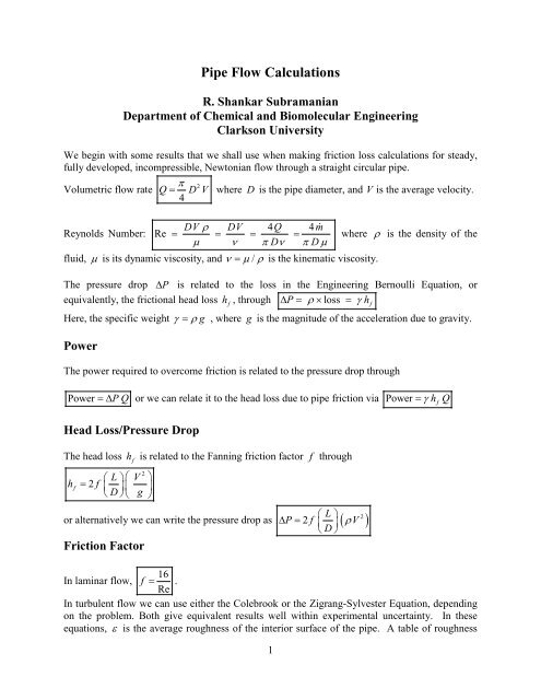
Pipe Flow Calculations - Clarkson University

Pipe Flow Calculations
R. Shankar Subramanian
Department of Chemical and Biomolecular Engineering
Clarkson University
We begin with some results that we shall use when making friction loss calculations for steady,
fully developed, incompressible, Newtonian flow through a straight circular pipe.
π 2
Volumetric flow rate Q= DV where D is the pipe diameter, and V is the average velocity.
4
DV ρ DV 4Q 4m
Reynolds Number: Re = = = = where ρ is the density of the
µ ν π Dν π Dµ
fluid, µ is its dynamic viscosity, and ν = µ / ρ is the kinematic viscosity.
The pressure drop ∆ P is related to the loss in the Engineering Bernoulli Equation, or
equivalently, the frictional head loss h
f
, through ∆ P= ρ× loss = γ hf
Here, the specific weight γ = ρ g , where g is the magnitude of the acceleration due to gravity.
Power
The power required to overcome friction is related to the pressure drop through
Power = ∆ PQ or we can relate it to the head loss due to pipe friction via Power = γ hf
Q
Head Loss/Pressure Drop
The head loss h
f
is related to the Fanning friction factor f through
h
f
2
⎛ L ⎞⎛ V ⎞
= 2 f ⎜ ⎟⎜ ⎟
⎝D⎠⎝ g ⎠
L
∆ = ⎜ ⎟
⎝D
⎠
⎛ ⎞ 2
or alternatively we can write the pressure drop as P 2 f ( ρ V )
Friction Factor
16
In laminar flow, f = .
Re
In turbulent flow we can use either the Colebrook or the Zigrang-Sylvester Equation, depending
on the problem. Both give equivalent results well within experimental uncertainty. In these
equations, ε is the average roughness of the interior surface of the pipe. A table of roughness
1

values recommended for commercial pipes given in a textbook on Fluid Mechanics by F.M.
White is provided at the end of these notes.
Colebrook Equation
1 ⎡ε
/ D 1.26
=− 4.0 log10
⎢ +
f
⎣⎢
3.7 Re f
⎤
⎥
⎦⎥
Zigrang-Sylvester Equation
1 ⎡ε
/ D 5.02 ⎛ε
/ D 13 ⎞⎤
=−4.0 log10 ⎢ − log10
⎜ + ⎟
f
3.7 Re 3.7 Re
⎥
⎣
⎝ ⎠⎦
Non-Circular Conduits
Not all flow conduits are circular pipes. An example of a non-circular cross-section in heat
exchanger applications is an annulus, which is the region between two circular pipes. Another is
a rectangular duct, used in HVAC (Heating, Ventilation, and Air-Conditioning) applications.
Less common are ducts of triangular or elliptical cross-sections, but they are used on occasion.
In all these cases, when the flow is turbulent, we use the same friction factor correlations that are
used for circular pipes, substituting an equivalent diameter for the pipe diameter. The equivalent
diameter D , which is set equal to four times the “Hydraulic Radius,” R is defined as follows.
e
h
D
e
Cross -Sectional Area
= 4Rh
= 4×
Wetted Perimeter
In this definition, the term “wetted perimeter” is used to designate the perimeter of the crosssection
that is in contact with the flowing fluid. This applies to a liquid that occupies part of a
conduit, as in sewer lines carrying waste-water, or a creek or river. If a gas flows through a
conduit, the entire perimeter is “wetted.”
Using the above definition, we arrive at the following results for the equivalent diameter for two
common cross-sections. We assume that the entire perimeter is “wetted.”
Rectangular Duct
b
a
For the duct shown in the sketch, the cross-sectional area is ab , while the perimeter is 2( a+
b)
so that the equivalent diameter is written as follows.
2

D
e
ab 2
= 4× =
2( a+ b)
⎛1 1⎞
⎜ + ⎟
⎝a
b⎠
If the flow is laminar, a result similar to that for circular tubes is available for the friction factor,
which can be written as f = C/ Re , where C is a constant that depends on the aspect ratio
a/
b, and the Reynolds number is defined using the equivalent diameter. A few values of the
constant C for selected values of the aspect ratio are given in the Table below (Source: F.M.
White, Fluid Mechanics, 7 th Edition). For other aspect ratios, you can use interpolation.
a/
b C a/
b C
1.0 14.23 6.0 19.70
1.33 14.47 8.0 20.59
2.0 15.55 10.0 21.17
2.5 16.37 20.0 22.48
4.0 18.23 ∞ 24.00
Annulus
a
b
The cross-sectional area of the annulus shown is ( a
2 b
2
)
2π ( a+ b)
. Therefore, the equivalent diameter is obtained as
2 2
( a − b )
π
De
= 4 = 2 a−
b
2π
( a+
b)
( )
π − , while the wetted perimeter is
Again, for laminar flow, we find that f = C/ Re , where C is a constant that depends on the
aspect ratio a/
b, and the Reynolds number is defined using the equivalent diameter. As with
the rectangular cross-section, a few values constant C for selected values of the aspect ratio are
given in the Table that follows (Source: F.M. White, Fluid Mechanics, 7 th Edition). For other
aspect ratios, you can use interpolation.
3

a/
b C a/
b C
1.0 24.00 10,0 22.34
1.25 23.98 20.0 21.57
1.67 23.90 100 20.03
2.5 23.68 1000 18.67
5.0 23.09 ∞ 16.00
Minor Losses
Minor losses is a term used to describe losses that occur in fittings, expansions, contractions, and
the like. Fittings commonly used in the industry include bends, tees, elbows, unions, and of
course, valves used to control flow. Even though these losses are called minor, they can be
substantial compared to those for flow through short straight pipe segments. Losses are
V
2 / 2g . Therefore, we can write
commonly reported in velocity heads. A velocity head is ( )
minor losses as
h
m
2
V
= KL
, where K
L
is called the loss coefficient.
2g
Typical values of K
L
for some common fittings are given below. Usually, the values depend
upon the nominal pipe diameter, the Reynolds number, and the manner in which the valve is
installed (screwed or flanged). Manufacturers’ data should be used wherever possible.
Globe Valve (fully open): 5.5 - 14
Gate Valve (fully open): 0.03 - 0.80
Swing Check Valve (fully open): 2.0 - 5.1
Standard 45 o Elbow: 0.2 - 0.4
Long radius 45 o Elbow: 0.14 - 0.21
Standard 90 o Elbow: 0.21 - 2.0
Long radius 90 o Elbow: 0.07 - 1.0
Tee: 0.1 - 2.4
When solving homework problems, use the values given in Table 13.1 in the textbook by
Welty et al.
Sudden Expansion and Sudden Contraction
A sudden expansion in a pipe is one of the few cases where the losses can be obtained from the
basic balances. The expression for K is given by
L
K
L
2
2
⎡ d ⎤
= ⎢1
−
2
D
⎥
⎣ ⎦
4

Here, d and D represent the diameters of the smaller and larger pipes, respectively. For a
sudden contraction, we can use the same result if d / D≥ 0.76 . For smaller values of d / D we
can use the empirical relation K = 0.42 ⎡1 − d / D ⎤
L
2 2
⎣ ⎦ .
In both cases, we should multiply K
L
by the velocity head in the pipe segment of diameter d .
The losses would be smaller if the expansion or contraction is gradual.
When a pipe empties into a reservoir, all the kinetic energy in the fluid coming in is dissipated,
so that you can treat this as a sudden expansion with the ratio d / D= 0, yielding K = 1.
Typical Pipe Flow Problems
In typical pipe flow problems, we know the nature of the fluid that will flow through the pipe,
and the temperature. Therefore, we can find the relevant physical properties immediately. They
are the density ρ and the dynamic viscosity µ . Knowing these properties, we also can calculate
the kinematic viscosity ν = µ / ρ.
The length of the pipe L can be estimated from process equipment layout considerations. The
nature of the fluid to be pumped will dictate corrosion constraints on the pipe material. Other
considerations are cost and ease of procurement. Based on these, we can select the material of
the pipe to be used, and once we do, the roughness ε can be specified. This leaves us with three
unspecified parameters, namely the head loss h
f
or equivalently, the pressure drop required to
pump the fluid ∆ p , the volumetric flow rate Q (or equivalently the mass flow rate), and the pipe
diameter D . Unless we plan to also optimize the cost, two of these must be specified, leaving
only a single parameter to be calculated. Thus, pipe flow problems that do not involve cost
optimization will fall into three broad categories.
1. Given D and Q , find the head loss h
f
L
2. Given D and h
f
, find the volumetric flow rate Q
3. Given Q and h
f
, find the diameter D
Each of these three types of problems is illustrated next with a numerical example.
5

Example 1
−4 2
Find the head loss due to the flow of 1,500 gpm of oil ( ν = 1.15× 10 ft / s ) through 1,600 feet
3
of 8" diameter cast iron pipe. If the density of the oil ρ = 1.75 slug / ft , what is the power to be
supplied by a pump to the fluid? Find the BHP of the pump if its efficiency is 0.85.
Solution
We have the following information.
3
−4 2
ρ = 1.75 slug / ft
ν = 1.15× 10 ft / s D = 0.667
ft
Therefore, the cross-sectional area is
( ) 2
A = πD / 4 = π× 0.667 ft / 4 = 0.349 ft
2 2
( )
1 ft / s ft
Q = 1500 ( gpm)
× = 3.34
448.8
s
3 3
( gpm)
Therefore, the average velocity through the pipe is V
We can calculate the Reynolds number.
3
( ft s)
2
( ft )
= Q 3.34 /
A
= 0.349
=
9.58
ft
s
( ft) × ( ft s)
DV 0.667 9.58 /
Re = = = 5.55×
10
ν
( ft s)
−4 2
1.15×
10 /
4
Therefore, the flow is turbulent.
−4
For cast iron, ε = 8.5 × 10 ft . Therefore, the relative roughness is
−4
( ft)
( ft)
ε 8.5 × 10
= = 1.27×
10
D 0.667
−3
Because we have the values of both the Reynolds number and the relative roughness, it is
efficient to use the Zigrang-Sylvester equation for a once-through calculation of the turbulent
flow friction factor.
1 ⎡ε
/ D 5.02 ⎛ε
/ D 13 ⎞⎤
=−4.0 log10 ⎢ − log10
⎜ + ⎟
3.7 Re 3.7 Re
⎥
f
⎣
⎝ ⎠⎦
−3 −3
⎡1.27× 10 5.02 ⎛1.27×
10 13 ⎞⎤
= −4.0 log10 ⎢ − log
4 10 ⎜ + 12.8
4 ⎟⎥
=
⎣ 3.7 5.55× 10 ⎝ 3.7 5.55×
10 ⎠⎦
which yields f = 0.00612
6

The head loss is obtained by using
( ft)
( )
( ft s)
2
⎛ L ⎞⎛ V ⎞
1,600 9.58 /
hf
= 2 f ⎜ ⎟⎜ ⎟= 2× 0.00612 × × = 83.7 ft
⎝D ⎠⎝ g ⎠
0.667 ft 32.2 ft / s
2
2
( )
⎛ ⎞ ⎛ ⎞
The mass flow rate is m
= ρ Q= 1.75 ⎜ × 3.34 = 5.85
⎝ ⎠ ⎝ ⎠
The power supplied to the fluid is calculated from
3
slug ft slug
3 ⎟ ⎜ ⎟
ft s s
⎛slug
⎞ ⎛ ft ⎞
ft • lb
4 f
Power to Fluid = m
hf
g = 5.85 ⎜ ⎟× 83.7 ( ft) × 32.2 ⎜ = 1.58 × 10
2 ⎟
⎝ s ⎠ ⎝s ⎠
s
ft • lb
We know that 1 HorsePower 550
f
= . Therefore, Power to Fluid = 28.7 hp
s
The efficiency of the pump η = 0.85 . Therefore,
28.7 ( hp)
Power to Fluid
Brake Horse Power = = = 33.7 hp
η 0.85
Example 2
Water at 15 C flows through a 25 − cm diameter riveted steel pipe of length 450 m and
roughness ε = 3.2 mm . The head loss is known to be 7.30 m . Find the volumetric flow rate of
water in the pipe.
Solution
For water at 15 C ,
ρ = 999 kg / m
−6 2
calculated as ν = µ / ρ = 1.16×
10 m / s
3
µ
−3
= 1.16× 10 Pa • s so that the kinematic viscosity can be
The pipe diameter is given as D= 0.25 m, so that the cross-sectional area is
( ) 2
A= πD / 4 = π× 0.25 m / 4 = 4.91×
10 m
2 −2 2
The length of the pipe is given as L=
450 m
We do not know the velocity of water in the pipe, but we can express the Reynolds number in
terms of the unknown velocity.
( m)
DV 0.25 × V
5
Re = = = 2.16×
10 V
ν ×
( m s)
−6 2
1.16 10 /
where V must be in m/
s.
At this point, we do not know whether the flow is laminar or turbulent. Given the size of the
pipe and the head loss, it is reasonable to assume turbulent flow and proceed. In the end, we
need to check whether this assumption is correct.
7

Now, we are given the head loss h
f
. Let us write the result for h
f
in terms of the friction factor.
2
⎛ L ⎞⎛ V ⎞
hf
= 2 f ⎜ ⎟⎜ ⎟ Substitute the values of known entities in this equation.
⎝D⎠⎝ g ⎠
2
⎛ 450 ( m)
⎞ ⎛ V ⎞
7.30 ( m)
= 2 f × 2
⎜ 0.25 ( m) ⎟ ×
This can be rearranged to yield
⎝ ⎠
⎜9.81 ( m/
s ) ⎟
⎝ ⎠
fV
2
m
= 1.99× 10 where V must be in m/
s.
2
s
2 −2
Taking the square root, we find
f
0.141
=
V
We can see that the product Re f can be calculated, even though we do not know the velocity
V .
Re f
5 0.141
4
= 2.16× 10 V × = 3.05×
10
V
Given ε = 3.2 mm , the relative roughness is
−3
ε 3.2×
10 ( m)
−2
= = 1.28×
10
D 0.25 m
( )
Therefore, the entire right side in the Colebrook Equation for the friction factor is known. We
can use the Colebrook Equation to evaluate the friction factor in an once-through calculation.
⎡ε
D ⎤ ⎡ ×
⎤
=− 4.0 log ⎢ + ⎥ =− 4.0 log 9.82
3.7
⎢ + =
Re f
3.7 3.05×
10
⎥
⎢⎣
⎥⎦
⎣ ⎦
−2
1 / 1.26 1.28 10 1.26
10 10 4
f
Therefore, the friction factor is f = 0.0104
0.141
Using f = , we can evaluate the velocity as
V
0.141 ( m/ s) 0.141 ( m/
s)
V = = = 1.39 m/
s so that the volumetric flow rate is obtained as
f 0.102
−
( ) ( )
Q = VA = 1.39 m / s × 4.91× 10 m = 6.80 × 10
2 2 −2
5 5
We must check the Reynolds number. Re = 2.16× 10 V = 3.00× 10 . This is well over 4,000
so that we can conclude that the assumption of turbulent flow is correct.
m
s
3
8

Example 3
Determine the size of smooth 14-gage BWG copper tubing needed to convey 10 gpm of a
−5 2
process liquid of kinematic viscosity ν = 2.40 × 10 ft / s over a distance of 133 ft at ground
level using a storage tank at an elevation of 20 ft . You can assume minor losses from fittings in
the line to account for 5 ft of head.
In this problem, we are asked to calculate the diameter D of the tube. We are given L = 150 ft
( )
3
1 ft / s
3
−2
ft
and Q = 10 gpm × = 2.23× 10 . Given that the storage tank is located at an
448.8( gpm)
s
elevation of 20 ft above ground, we can infer that the available head loss for friction in the flow
h = 20 − 5 ft = 15 ft .
through the tube is ( )
f
The diameter appears in both the Reynolds number and the result for the head loss in terms of the
friction factor. Let us begin with the head loss and write it in terms of the volumetric flow rate,
which is known.
2
( Q π D ) 2
⎛ 4 / ⎞
⎛ L ⎞⎛
V ⎞ ⎛ L ⎞ 32 LQ
hf
= 2f 2f ⎜ ⎟
⎜ ⎟⎜
⎟= ⎜ ⎟ = f ×
⎝D ⎠⎝
g ⎠ ⎝D ⎠ ⎜ g ⎟ π gD
⎝
⎠
2 2
Substituting known entities in this equation, we obtain
2 5
−2 3
( ) ( )
× 32.2 ( ft / s ) × D
32× 133 ft × 2.23×
10 ft / s
−3
f
15 ft = f × = 6.65×
10
2 2 5
π
D
where D must be in feet.
2
5
so that
f
= 2.26×
10
D
3 5
The Reynolds number can be written as
( ft s)
( )
4Q
4× 2.23× 10 / 1.18×
10
Re = = =
πνD
π × × ft s × D D
−5 2
2.40 10 /
−2 3 3
9
where D must be in feet.
We can make further progress if we assume the type of flow, so that we can use a correlation for
the friction factor. It is reasonable in process situations with this flow rate to assume turbulent
flow. So, we shall proceed with that assumption, to be verified later when we can calculate the
Reynolds number.
It does not matter which correlation we use, because we must solve an implicit equation for the
diameter in either case. So, let us use the Colebrook equation because it is simpler. For a
smooth tube, the roughness , ε = 0 , so that we can set the relative roughness ε / D = 0 in the
Colebrook equation to obtain

1 ⎡ 1.26 ⎤
= − 4.0 log10
⎢ ⎥
f
⎢⎣Re
f ⎥⎦
In this equation, substitute for both the friction factor and the Reynolds number in terms of the
diameter, to obtain
⎡ ⎤ −5
⎡ × ⎤
4.0 log
5/2 10
⎢
⎥ 4.0 log10
3/2
1 1.26 2.25 10
=− =−
3 5/2
47.5D
⎢
( 1.18 10 / D) ( 47.5 D )
D
⎥
⎢⎣
× × ⎥⎦
⎣ ⎦
or
D
=− 190 log ⎡
⎣2.25×
10
D
−5/2 −5 −3/2
10
⎤
⎦
Solving this equation, we obtain
−2
7.91 10 0.949"
D = × ft =
A table of standard tubing dimensions for specified nominal diameters and Birmingham Wire
Gage (BWG) values can be found in many places. The textbook by Welty et al. provides it as
Appendix N. From the table, we find that for 14-gage tubing with an outside diameter of 1" , the
1
inside diameter is 0.834”. The next higher outside diameter available is 1 − inch , and for this
4
OD, 14-gage tubing comes with an inside diameter of 1.084”. Therefore, we must select one of
these two tubes. If we want to be sure to obtain the desired flow rate, we must choose the value
that is larger than 0.949” . You may wonder why. Here is an approximate answer.
In turbulent flow, the friction factor f ∝ V −a , where 0≤
a < 1. In laminar flow, f ∝ V −1 . In
2 b
both cases, we can write fV ∝ V where b > 0 . Therefore, the head loss from pipe flow
1 2⎛2L
⎞ 1 2 1 b
friction hf
= fV ⎜ ⎟∝ fV ∝ V
D ⎝ g ⎠ D D
For a fixed volumetric flow rate, as the diameter is increased, V b decreases and 1/ D also
decreases. Therefore, the head loss decreases for a given volumetric flow rate as the diameter is
increased. This means that with a fixed head loss available, we can comfortably achieve the
desired flow rate using a suitable valve. On the other hand, if we choose a diameter that is
smaller than the calculated value, we would need a larger head available for driving the flow
than is available.
Now, let us use the actual inside diameter of the selected tube,
evaluate the Reynolds number of the flow.
D
−2
= 1.084" = 9.03× 10 ft to
10

−2 3
( ft s)
−
( ) ( )
4Q
4× 2.23×
10 /
Re = = = 1.31×
10
πν
−5 2 2
D π × 2.40 × 10 ft / s × 9.03×
10 ft
turbulent as assumed.
4
Therefore, the flow is
The actual friction factor can be calculated from the Zigrang-Sylvester equation.
1 ⎡ε
/ D 5.02 ⎛ε
/ D 13 ⎞⎤
=−4.0 log10 ⎢ − log10
⎜ + ⎟
3.7 Re 3.7 Re
⎥
f
⎣
⎝ ⎠⎦
⎡ 5.02 ⎛ 13 ⎞⎤
= −4.0 log10 ⎢0 − log
4 10 ⎜0 + 11.8
4 ⎟ =
1.31× 10 1.31×
10
⎥
⎣
⎝
⎠⎦
yielding f = 0.00724
The actual head loss for the desired volumetric flow rate will be
−2 3
2
( ft) ( ft s)
−
( ) ( )
2
32 LQ
32× 133 × 2.23×
10 /
hf
= f × 0.00724 8.03
2 gD = × = ft
5
2 2 2
5
π
π × 32.2 ft / s × 9.03×
10 ft
which is less than available head of 15 ft .
Therefore, we must specify 14-gage,
1
1 4
− inch tubing for this application.
11

Roughness values for Commercial Pipes
These roughness values are given in Table 6.1 from a textbook by White (1). Because of the
variation in roughness in these materials depending on the source, the roughness values reported
here have uncertainties ranging from ± 20 % for new wrought Iron to ± 70 % for riveted steel.
A typical uncertainty in the roughness values can be assumed to be in the range ± 30 − 50 % .
Material Condition ft mm
Steel Sheet metal, new
4
1.6×
10 −
5×
10 −2
Stainless, new
6
7×
10 −
2×
10 −3
Commercial, new
4
1.5×
10 −
4.6×
10 −2
Riveted
2
1× 10 −
3.0
Rusted
3
7× 10 −
2.0
Iron Cast, new
4
8.5×
10 −
2.6×
10 −1
Wrought, new
4
1.5×
10 −
4.6×
10 −2
Galvanized, new
4
5×
10 −
1.5×
10 −1
Asphalted, cast
4
4×
10 −
1.2×
10 −1
Brass Drawn, new
6
7×
10 −
2×
10 −3
Plastic Drawn tubing
6
5×
10 −
1.5×
10 −3
Glass Smooth Smooth
Concrete Smoothed
4
1.3×
10 −
4×
10 −2
Rough
3
7× 10 −
2.0
Rubber Smoothed
5
3.3×
10 −
1×
10 −2
Wood Stave
3
1.6×
10 −
5×
10 −1
Reference
1. F.M. White, Fluid Mechanics, 7 th Edition, McGraw-Hill, New York, 2011.
12