Kahn Process Networks and Dataflows - Chess
Kahn Process Networks and Dataflows - Chess
Kahn Process Networks and Dataflows - Chess
You also want an ePaper? Increase the reach of your titles
YUMPU automatically turns print PDFs into web optimized ePapers that Google loves.
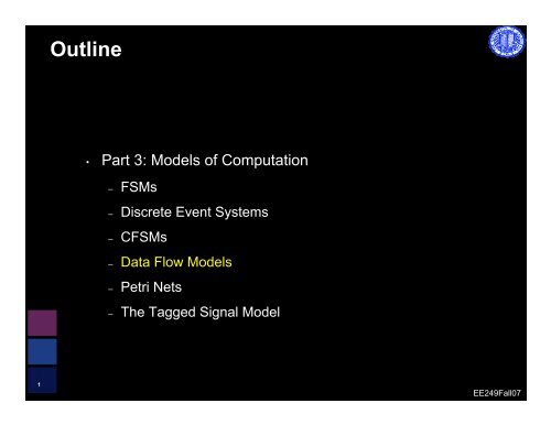
Outline<br />
• Part 3: Models of Computation<br />
– FSMs<br />
– Discrete Event Systems<br />
– CFSMs<br />
– Data Flow Models<br />
– Petri Nets<br />
– The Tagged Signal Model<br />
1<br />
EE249Fall07
Data-flow networks<br />
• A bit of history<br />
• Syntax <strong>and</strong> semantics<br />
– actors, tokens <strong>and</strong> firings<br />
• Scheduling of Static Data-flow<br />
– static scheduling<br />
– code generation<br />
– buffer sizing<br />
• Other Data-flow models<br />
– Boolean Data-flow<br />
– Dynamic Data-flow<br />
2<br />
EE249Fall07
Data-flow networks<br />
• Powerful formalism for data-dominated system specification<br />
• Partially-ordered model (no over-specification)<br />
• Deterministic execution independent of scheduling<br />
• Used for<br />
– simulation<br />
– scheduling<br />
– memory allocation<br />
– code generation<br />
for Digital Signal <strong>Process</strong>ors (HW <strong>and</strong> SW)<br />
3<br />
EE249Fall07
A bit of history<br />
• Karp computation graphs (‘66): seminal work<br />
• <strong>Kahn</strong> process networks (‘58): formal model<br />
• Dennis Data-flow networks (‘75): programming language for MIT<br />
DF machine<br />
• Several recent implementations<br />
– graphical:<br />
– Ptolemy (UCB), Khoros (U. New Mexico), Grape (U. Leuven)<br />
– SPW (Cadence), COSSAP (Synopsys)<br />
– textual:<br />
– Silage (UCB, Mentor)<br />
– Lucid, Haskell<br />
4<br />
EE249Fall07
Data-flow network<br />
• A Data-flow network is a collection of functional nodes which<br />
are connected <strong>and</strong> communicate over unbounded FIFO queues<br />
• Nodes are commonly called actors<br />
• The bits of information that are communicated over the queues<br />
are commonly called tokens<br />
5<br />
EE249Fall07
Intuitive semantics<br />
• (Often stateless) actors perform computation<br />
• Unbounded FIFOs perform communication via sequences of<br />
tokens carrying values<br />
– integer, float, fixed point<br />
– matrix of integer, float, fixed point<br />
– image of pixels<br />
• State implemented as self-loop<br />
• Determinacy:<br />
– unique output sequences given unique input sequences<br />
– Sufficient condition: blocking read<br />
– (process cannot test input queues for emptiness)<br />
6<br />
EE249Fall07
Intuitive semantics<br />
• At each time, one actor is fired<br />
• When firing, actors consume input tokens <strong>and</strong> produce output<br />
tokens<br />
• Actors can be fired only if there are enough tokens in the input<br />
queues<br />
7<br />
EE249Fall07
Intuitive semantics<br />
• Example: FIR filter<br />
– single input sequence i(n)<br />
– single output sequence o(n)<br />
– o(n) = c1 i(n) + c2 i(n-1)<br />
i<br />
* c2<br />
* c1<br />
i(-1)<br />
8<br />
+ o<br />
EE249Fall07
Intuitive semantics<br />
• Example: FIR filter<br />
– single input sequence i(n)<br />
– single output sequence o(n)<br />
– o(n) = c1 i(n) + c2 i(n-1)<br />
i<br />
* c2<br />
* c1<br />
i(-1)<br />
9<br />
+ o<br />
EE249Fall07
Intuitive semantics<br />
• Example: FIR filter<br />
– single input sequence i(n)<br />
– single output sequence o(n)<br />
– o(n) = c1 i(n) + c2 i(n-1)<br />
i<br />
* c2<br />
* c1<br />
i(-1)<br />
10<br />
+ o<br />
EE249Fall07
Intuitive semantics<br />
• Example: FIR filter<br />
– single input sequence i(n)<br />
– single output sequence o(n)<br />
– o(n) = c1 i(n) + c2 i(n-1)<br />
i<br />
* c2<br />
* c1<br />
i(-1)<br />
11<br />
+ o<br />
EE249Fall07
Intuitive semantics<br />
• Example: FIR filter<br />
– single input sequence i(n)<br />
– single output sequence o(n)<br />
– o(n) = c1 i(n) + c2 i(n-1)<br />
i<br />
* c2<br />
* c1<br />
i(-1)<br />
12<br />
+ o<br />
EE249Fall07
Intuitive semantics<br />
• Example: FIR filter<br />
– single input sequence i(n)<br />
– single output sequence o(n)<br />
– o(n) = c1 i(n) + c2 i(n-1)<br />
i<br />
* c2<br />
* c1<br />
i(-1)<br />
13<br />
+ o<br />
EE249Fall07
Intuitive semantics<br />
• Example: FIR filter<br />
– single input sequence i(n)<br />
– single output sequence o(n)<br />
– o(n) = c1 i(n) + c2 i(n-1)<br />
i<br />
* c2<br />
* c1<br />
14<br />
+ o<br />
EE249Fall07
Intuitive semantics<br />
• Example: FIR filter<br />
– single input sequence i(n)<br />
– single output sequence o(n)<br />
– o(n) = c1 i(n) + c2 i(n-1)<br />
i<br />
* c2<br />
* c1<br />
15<br />
+ o<br />
EE249Fall07
Intuitive semantics<br />
• Example: FIR filter<br />
– single input sequence i(n)<br />
– single output sequence o(n)<br />
– o(n) = c1 i(n) + c2 i(n-1)<br />
i<br />
* c2<br />
* c1<br />
16<br />
+ o<br />
EE249Fall07
Intuitive semantics<br />
• Example: FIR filter<br />
– single input sequence i(n)<br />
– single output sequence o(n)<br />
– o(n) = c1 i(n) + c2 i(n-1)<br />
i<br />
* c2<br />
* c1<br />
17<br />
+ o<br />
EE249Fall07
Questions<br />
• Does the order in which actors are fired affect the final result?<br />
• Does it affect the “operation” of the network in any way?<br />
• Go to Radio Shack <strong>and</strong> ask for an unbounded queue!!<br />
18<br />
EE249Fall07
Formal semantics: sequences<br />
• Actors operate from a sequence of input tokens to a sequence of<br />
output tokens<br />
• Let tokens be noted by x 1 , x 2 , x 3 , etc…<br />
• A sequence of tokens is defined as<br />
X = [ x 1 , x 2 , x 3 , …]<br />
• Over the execution of the network, each queue will grow a particular<br />
sequence of tokens<br />
• In general, we consider the actors mathematically as functions from<br />
sequences to sequences (not from tokens to tokens)<br />
19<br />
EE249Fall07
Ordering of sequences<br />
• Let X 1 <strong>and</strong> X 2 be two sequences of tokens.<br />
• We say that X 1 is less than X 2 if <strong>and</strong> only if (by definition) X 1 is<br />
an initial segment of X 2<br />
• Homework: prove that the relation so defined is a partial order<br />
(reflexive, antisymmetric <strong>and</strong> transitive)<br />
• This is also called the prefix order<br />
• Example: [ x 1 , x 2 ]
Chains of sequences<br />
• Consider the set S of all finite <strong>and</strong> infinite sequences of<br />
tokens<br />
• This set is partially ordered by the prefix order<br />
• A subset C of S is called a chain iff all pairs of elements of C<br />
are comparable<br />
• If C is a chain, then it must be a linear order inside S<br />
(otherwise, why call it chain?)<br />
• Example: { [ x 1 ], [ x 1 , x 2 ], [ x 1 , x 2 , x 3 ], … } is a chain<br />
• Example: { [ x 1 ], [ x 1 , x 2 ], [ x 1 , x 3 ], … } is not a chain<br />
21<br />
EE249Fall07
(Least) Upper Bound<br />
• Given a subset Y of S, an upper bound of Y is an element z of<br />
S such that z is larger than all elements of Y<br />
• Consider now the set Z (subset of S) of all the upper bounds<br />
of Y<br />
• If Z has a least element u, then u is called the least upper<br />
bound (lub) of Y<br />
• The least upper bound, if it exists, is unique<br />
• Note: u might not be in Y (if it is, then it is the largest value of<br />
Y)<br />
22<br />
EE249Fall07
Complete Partial Order<br />
• Every chain in S has a least upper bound<br />
• Because of this property, S is called a Complete Partial Order<br />
• Notation: if C is a chain, we indicate the least upper bound of<br />
C by lub( C )<br />
• Note: the least upper bound may be thought of as the limit of<br />
the chain<br />
23<br />
EE249Fall07
<strong>Process</strong>es<br />
• <strong>Process</strong>: function from a p-tuple of sequences to a q-tuple of<br />
sequences<br />
F : S p -> S q<br />
• Tuples have the induced point-wise order:<br />
Y = ( y 1 , … , y p ), Y’ = ( y’ 1 , … , y’ p ) in S p :Y
Continuity <strong>and</strong> Monotonicity<br />
• Continuity: F is continuous iff (by definition) for all chains C,<br />
lub( F( C ) ) exists <strong>and</strong><br />
F( lub( C ) = lub( F( C ) )<br />
• Similar to continuity in analysis using limits<br />
• Monotonicity: F is monotonic iff (by definition) for all pairs X, X’<br />
X F( X )
Least Fixed Point semantics<br />
• Let X be the set of all sequences<br />
• A network is a mapping F from the sequences to the<br />
sequences<br />
X = F( X, I )<br />
• The behavior of the network is defined as the unique least<br />
fixed point of the equation<br />
• If F is continuous then the least fixed point exists LFP =<br />
LUB( { F n ( ⊥, I ) : n >= 0 } )<br />
26<br />
EE249Fall07
From <strong>Kahn</strong> networks to Data Flow networks<br />
• Each process becomes an actor: set of pairs of<br />
– firing rule<br />
(number of required tokens on inputs)<br />
– function<br />
(including number of consumed <strong>and</strong> produced tokens)<br />
• Formally shown to be equivalent, but actors with firing are<br />
more intuitive<br />
• Mutually exclusive firing rules imply monotonicity<br />
• Generally simplified to blocking read<br />
27<br />
EE249Fall07
Examples of Data Flow actors<br />
• SDF: Synchronous (or, better, Static) Data Flow<br />
– fixed input <strong>and</strong> output tokens<br />
1<br />
1<br />
+<br />
1<br />
FFT<br />
1024 1024 10 1<br />
• BDF: Boolean Data Flow<br />
– control token determines consumed <strong>and</strong> produced tokens<br />
28<br />
T<br />
merge<br />
F<br />
T<br />
select<br />
F<br />
EE249Fall07
Static scheduling of DF<br />
• Key property of DF networks: output sequences do not depend on<br />
time of firing of actors<br />
• SDF networks can be statically scheduled at compile-time<br />
– execute an actor when it is known to be fireable<br />
– no overhead due to sequencing of concurrency<br />
– static buffer sizing<br />
• Different schedules yield different<br />
– code size<br />
– buffer size<br />
– pipeline utilization<br />
29<br />
EE249Fall07
Static scheduling of SDF<br />
• Based only on process graph (ignores functionality)<br />
• Network state: number of tokens in FIFOs<br />
• Objective: find schedule that is valid, i.e.:<br />
– admissible<br />
(only fires actors when fireable)<br />
– periodic<br />
(brings network back to initial state firing each actor at least once)<br />
• Optimize cost function over admissible schedules<br />
30<br />
EE249Fall07
Balance equations<br />
• Number of produced tokens must equal number of consumed tokens<br />
on every edge<br />
A<br />
n p<br />
n c<br />
B<br />
• Repetitions (or firing) vector v S of schedule S: number of firings of<br />
each actor in S<br />
• v S (A) n p = v S (B) n c<br />
must be satisfied for each edge<br />
31<br />
EE249Fall07
Balance equations<br />
1<br />
B<br />
3<br />
1<br />
A<br />
2<br />
2<br />
1<br />
1<br />
1<br />
C<br />
• Balance for each edge:<br />
– 3 v S (A) - v S (B) = 0<br />
– v S (B) - v S (C) = 0<br />
– 2 v S (A) - v S (C) = 0<br />
– 2 v S (A) - v S (C) = 0<br />
32<br />
EE249Fall07
Balance equations<br />
1<br />
B<br />
3<br />
1<br />
A<br />
2<br />
2<br />
1<br />
1<br />
1<br />
C<br />
M =<br />
3 -1 0<br />
0 1 -1<br />
2 0 -1<br />
2 0 -1<br />
• M v S = 0<br />
iff S is periodic<br />
• Full rank (as in this case)<br />
– no non-zero solution<br />
– no periodic schedule<br />
(too many tokens accumulate on A->B or B->C)<br />
33<br />
EE249Fall07
Balance equations<br />
1<br />
B<br />
2<br />
1<br />
A<br />
2<br />
2<br />
1<br />
1<br />
1<br />
C<br />
M =<br />
2 -1 0<br />
0 1 -1<br />
2 0 -1<br />
2 0 -1<br />
• Non-full rank<br />
– infinite solutions exist (linear space of dimension 1)<br />
• Any multiple of q = |1 2 2| T satisfies the balance equations<br />
• ABCBC <strong>and</strong> ABBCC are minimal valid schedules<br />
• ABABBCBCCC is non-minimal valid schedule<br />
34<br />
EE249Fall07
Static SDF scheduling<br />
• Main SDF scheduling theorem (Lee ‘86):<br />
– A connected SDF graph with n actors has a periodic schedule iff its<br />
topology matrix M has rank n-1<br />
– If M has rank n-1 then there exists a unique smallest integer solution q<br />
to<br />
M q = 0<br />
• Rank must be at least n-1 because we need at least n-1 edges<br />
(connected-ness), providing each a linearly independent row<br />
• Admissibility is not guaranteed, <strong>and</strong> depends on initial tokens on<br />
cycles<br />
35<br />
EE249Fall07
Admissibility of schedules<br />
1<br />
A<br />
2<br />
1<br />
3<br />
B<br />
2<br />
3<br />
C<br />
• No admissible schedule:<br />
BACBA, then deadlock…<br />
• Adding one token (delay) on A->C makes<br />
BACBACBA valid<br />
• Making a periodic schedule admissible is always possible, but<br />
changes specification...<br />
36<br />
EE249Fall07
Admissibility of schedules<br />
• Adding initial token changes FIR order<br />
i<br />
i(-1)<br />
i(-2)<br />
* c1<br />
* c2<br />
+ o<br />
37<br />
EE249Fall07
From repetition vector to schedule<br />
• Repeatedly schedule fireable actors up to number of times in<br />
repetition vector<br />
q = |1 2 2| T<br />
1<br />
B<br />
2<br />
1<br />
A<br />
2<br />
2<br />
1<br />
1<br />
1<br />
C<br />
• Can find either ABCBC or ABBCC<br />
• If deadlock before original state, no valid schedule exists (Lee ‘86)<br />
38<br />
EE249Fall07
From schedule to implementation<br />
• Static scheduling used for:<br />
– behavioral simulation of DF (extremely efficient)<br />
– code generation for DSP<br />
– HW synthesis (Cathedral by IMEC, Lager by UCB, …)<br />
• Issues in code generation<br />
– execution speed (pipelining, vectorization)<br />
– code size minimization<br />
– data memory size minimization (allocation to FIFOs)<br />
– processor or functional unit allocation<br />
39<br />
EE249Fall07
Compilation optimization<br />
• Assumption: code stitching<br />
(chaining custom code for each actor)<br />
• More efficient than C compiler for DSP<br />
• Comparable to h<strong>and</strong>-coding in some cases<br />
• Explicit parallelism, no artificial control dependencies<br />
• Main problem: memory <strong>and</strong> processor/FU allocation<br />
depends on scheduling, <strong>and</strong> vice-versa<br />
40<br />
EE249Fall07
Code size minimization<br />
• Assumptions (based on DSP architecture):<br />
– subroutine calls expensive<br />
– fixed iteration loops are cheap<br />
(“zero-overhead loops”)<br />
• Absolute optimum: single appearance schedule<br />
e.g. ABCBC -> A (2BC), ABBCC -> A (2B) (2C)<br />
– may or may not exist for an SDF graph…<br />
– buffer minimization relative to single appearance schedules<br />
(Bhattacharyya ‘94, Lauwereins ‘96, Murthy ‘97)<br />
41<br />
EE249Fall07
Buffer size minimization<br />
• Assumption: no buffer sharing<br />
• Example:<br />
A<br />
1<br />
10<br />
B<br />
1<br />
10<br />
C<br />
1 10<br />
D<br />
q = | 100 100 10 1| T<br />
• Valid SAS: (100 A) (100 B) (10 C) D<br />
– requires 210 units of buffer area<br />
• Better (factored) SAS: (10 (10 A) (10 B) C) D<br />
– requires 30 units of buffer areas, but…<br />
– requires 21 loop initiations per period (instead of 3)<br />
42<br />
EE249Fall07
Dynamic scheduling of DF<br />
• SDF is limited in modeling power<br />
– no run-time choice<br />
– cannot implement Gaussian elimination with pivoting<br />
• More general DF is too powerful<br />
– non-Static DF is Turing-complete (Buck ‘93)<br />
– bounded-memory scheduling is not always possible<br />
• BDF: semi-static scheduling of special “patterns”<br />
– if-then-else<br />
– repeat-until, do-while<br />
• General case: thread-based dynamic scheduling<br />
– (Parks ‘96: may not terminate, but never fails if feasible)<br />
43<br />
EE249Fall07
Example of Boolean DF<br />
• Compute absolute value of average of n samples<br />
0<br />
0<br />
T<br />
>n<br />
T F T F<br />
T<br />
+1 +<br />
In<br />
Example of general DF<br />
• Merge streams of multiples of 2 <strong>and</strong> 3 in order (removing duplicates)<br />
45<br />
* 2 dup<br />
1<br />
• Deterministic merge<br />
(no “peeking”)<br />
A<br />
* 3 dup<br />
1<br />
ordered<br />
merge<br />
O<br />
out<br />
B<br />
a = get (A)<br />
b = get (B)<br />
forever {<br />
if (a > b) {<br />
put (O, a)<br />
a = get (A)<br />
} else if (a < b) {<br />
put (O, b)<br />
b = get (B)<br />
} else {<br />
put (O, a)<br />
a = get (A)<br />
b = get (B)<br />
}<br />
}<br />
EE249Fall07
Summary of DF networks<br />
• Advantages:<br />
– Easy to use (graphical languages)<br />
– Powerful algorithms for<br />
– verification (fast behavioral simulation)<br />
– synthesis (scheduling <strong>and</strong> allocation)<br />
– Explicit concurrency<br />
• Disadvantages:<br />
– Efficient synthesis only for restricted models<br />
– (no input or output choice)<br />
– Cannot describe reactive control (blocking read)<br />
46<br />
EE249Fall07
Base-b<strong>and</strong> <strong>Process</strong>ing in Cell Phones<br />
Frame to transmit<br />
(stream of bits)<br />
Preprocessing<br />
Add headers etc.<br />
End<br />
of Pkt<br />
Payload<br />
Network<br />
information<br />
Synch<br />
Mapping on a<br />
Constellation (QPSK)<br />
Filtering<br />
Modulation<br />
47<br />
EE249Fall06
Base-b<strong>and</strong> <strong>Process</strong>ing: Denotation<br />
Composition of functions = overall base-b<strong>and</strong> specification<br />
Mapping on a<br />
Constellation (QPSK)<br />
Filtering<br />
Modulation<br />
48<br />
EE249Fall06
Base-b<strong>and</strong> <strong>Process</strong>ing: Data Flow Model<br />
RRC<br />
Mult<br />
MAP<br />
Sum<br />
RRC<br />
Mult<br />
Mapping on a<br />
Constellation (QPSK)<br />
Filtering<br />
Modulation<br />
49<br />
EE249Fall06
Remarks<br />
• Composition is achieved by input-output connection through<br />
communication channels (FIFOs)<br />
• The operational semantics dictates the conditions that must be<br />
satisfied to execute a function (actor)<br />
• Functions operating on streams of data rather than states<br />
evolving in response to traces of events (data vs. control)<br />
• Convenient to mix denotational <strong>and</strong> operational specifications<br />
50<br />
EE249Fall07
Telecom/MM applications<br />
• Heterogeneous specifications including<br />
– data processing<br />
– control functions<br />
• Data processing, e.g. encryption, error correction…<br />
– computations done at regular (often short) intervals<br />
– efficiently specified <strong>and</strong> synthesized using DataFlow models<br />
• Control functions (data-dependent <strong>and</strong> real-time)<br />
– say when <strong>and</strong> how data computation is done<br />
– efficiently specified <strong>and</strong> synthesized using FSM models<br />
• Need a common model to perform global system analysis <strong>and</strong><br />
optimization<br />
51<br />
EE249Fall07
Mixing the two models: 802.11b<br />
• State machine for control<br />
– Denotational: processes as sequence of events, sequential<br />
composition, choice etc.<br />
– Operational: state transition graphs<br />
• Data Flow for signal processing<br />
– Functions<br />
– Data flow graphs<br />
• And what happens when we put them together?<br />
52<br />
EE249Fall07
802.11b: Modes of operation<br />
Data rate Modulation Coding Ndbps 1472 byte<br />
(Mbit/s) rate transfer duration(µs)<br />
<br />
<br />
6 BPSK 1/2 24 2012<br />
9 BPSK 3/4 36 1344<br />
12 QPSK 1/2 48 1008<br />
18 QPSK 3/4 72 672<br />
24 16-QAM 1/2 96 504<br />
36 16-QAM 3/4 144 336<br />
48 64-QAM 2/3 192 252<br />
54 64-QAM 3/4 216 224<br />
Channel<br />
estimation<br />
RX<br />
• Depending on the channel conditions, the modulation scheme changes<br />
• It is natural to mix FSM <strong>and</strong> DF (like in figure)<br />
Link<br />
quality<br />
Mode<br />
FSM<br />
Multimode<br />
Modulator<br />
• Note that now we have real-time constraints on this system (i.e. time to<br />
send 1472 bytes)<br />
TX<br />
53<br />
EE249Fall07
Outline<br />
• Part 3: Models of Computation<br />
– FSMs<br />
– Discrete Event Systems<br />
– CFSMs<br />
– Data Flow Models<br />
– Petri Nets<br />
– The Tagged Signal Model<br />
54<br />
EE249Fall07


