Ph.D. thesis (pdf) - dirac

THÈSE
présentée par
Kristine NISS
pour obtenir le grade de DOCTEUR
DE L’UNIVERSITÉ
DE PARIS XI
spécialité CHIMIE PHYSIQUE
Fast and slow dynamics of glass-forming liquids
–
What can we learn from high pressure experiments?
Soutenue le 19 Janvier 2007 devant le jury composé de:
Rapporteurs: Dr. Catherine Dreyfus
Dr. Helmut Schober
Prof. Giancarlo Ruocco
Dr. Jean-Philippe Bouchaud
Prof. Mehran Mostafavi
Prof. Jeppe Dyre
Directrice de thèse: Dr. Christiane Alba-Simionesco

Abstract
The focus in this study is on the fragility concept, that is the degree of departure
from Arrhenius temperature dependence of the relaxation time in the viscous liquid.
Fragility has in the course of the last decade been shown to (or suggested to) correlate
with a large number of properties in the liquid and the corresponding glass. We
develop a set of criteria for scrutinizing these types of correlations by introducing
pressure as a control variable in addition to temperature. Particularly we show that
correlations to isobaric fragility can be either signatures of a relation to the effect of
density on the relaxation time, or on the relation to the temperature dependence of
the relaxation time, or to a balanced combination of the two.
These criteria are used in the analysis of an extensive new set of data on the temperature
and pressure dependence of a number of different dynamical variables in
molecular and polymeric glass-forming systems. We particularly study the width of
the alpha relaxation by dielectric spectroscopy, the relative intensity of the boson
peak and the mean square displacement by neutron scattering and the nonergodicity
factor by inelastic X-ray scattering.
In the study of the width of the alpha relaxation as well as the relative intensity
of the boson peak we find that they do not relate to the effect of density on the
relaxation time, and that a physically meaningful correlation in these cases should be
a correlation to isochoric fragility rather than to the conventional isobaric fragility.
The mean square displacement is found to relate to a balanced combination of
temperature and density, while we suggest that the nonergodicity factor evaluated
at T g is correlated with the relative effect of density on the viscous slowing down.
iii

Acknowledgement
First of all I would like to sincerely thank my supervisor Christiane Alba-Simionesco
for letting me be her apprentice in the most genuine sense of the word; sharing,
challenging and inspiring in science and in life. Secondly I owe a special thank
to my companion and successor Cécile Dalle-Ferrier for her enormous moral and
practical support.
I am grateful to Gilles Tarjus for always making things clearer and to Bernhard Frick
for introducing me to the art and craft of neutron scattering. I am also thankful for
fruitful discussions and collaborations with numerous other researches and I would
particularly like to express my gratitude to : Alexei Sokolov, Vladimir Novikov,
Jeppe Dyre, Niels Boye Olsen, Uli Buchenau and Tullio Scopigno. Moreover I would
like to thank my jury and particularly the two rapportuers, Helmuth Schober and
Cathrine Dreyfus, for the many useful comments and intriguing questions.
The work presented in this thesis has been carried out at the Laboratoire de Chimie
Physique (LCP) in Orsay from January 2004 to December 2006, and I thank the
former and present director, Alain Fuchs and Mehran Mostafavi for hosting me.
The INS experiments were performed at ILL and were only possible thanks to the
staff on IN5, IN10 and the pressurelab : Jacques Ollivier, Luis Melesi, Tilo Seydel,
Matthias Elender and Steve Jenkins.
The IXS measurements were made possible thanks to the staff on ID16 and ID28 :
Michael Krisch, Roberto Verbeni and Alexandre Beraud. I am particularly grateful
to Giulio Monaco for his help with the data treatment and for many inspiring
discussions.
I would also like to thank Claudio Masciovecchio, Silvia Santucci and Allesandro
Gessini for an enlightening week on the IUVS beam-line on ELETTRA.
The development and fabrication of the dielectric spectroscopy setup at LCP was
made possible thanks to the expertise and efficiency technical staff at LCP, I would
particularly like to acknowledge the work of Joél Jaffrë, Jean-Robert Bazouin an
v

vi
Acknowledgement
Raymond Herren. The technical assistance and help of the staff at IMFUFA has
also been indispensable for this work and I thank Ib Hst Petersen, Peter Jensen and
Ebbe Hyldahl Larsen.
A special thank also goes to Jens Christian Niss for proofreading the whole manuscript
in a very short time.
Albena Nielsen and coworkers are thanked for making available dielectric data prior
to publication and I would at the same time like to thank every one in “Glass and
Time” (Denmark) for moral support.
My three years in the TESMaC group have been a real pleasure, and I am greatly
thankful to everyone for helping me out, supporting me and being overbearing with
my French. I would especially like to thank Jean-Marie Teuler for solving at least
million software problems, and Anne Boutin for strong support when it was most
needed. I would also like to thank the former Ph.D.-student Aude Chauty-Cailliaux,
from whom I overtook many results and experiences.
Finally I would like to thank ...
Maj and Bo for being present at all times no matter how far away (and for coming
closer). Niels for being there at the best (or worst) time possible. Paola, Carmelo,
Elisa, Javier and Kosima for making Grenoble feel like a second home. Christelle,
Angela, Ricardo, Aurelie, Frederic, Silvian, Gilbert, Pernille, Jean Luc, Margrethe,
Stephan, Lucie, Anders, Guara and all of ECAP for making Paris home. And all
my other friends and my family - I am grateful that they are far too numerous to
be listed here.
Kristine Niss April 2007
This work was supported by grant No. 645-03-0230
from Forskeruddannelsesrådet (Denmark).

Contents
Abstract
iii
Acknowledgement
v
1 Introduction 1
2 Slow and fast dynamics 7
2.1 The glass transition . . . . . . . . . . . . . . . . . . . . . . . . . . . 7
2.2 Fragility . . . . . . . . . . . . . . . . . . . . . . . . . . . . . . . . . . 10
2.3 Non-Debye relaxation . . . . . . . . . . . . . . . . . . . . . . . . . . 13
2.4 Energy landscape . . . . . . . . . . . . . . . . . . . . . . . . . . . . . 14
2.5 Fast dynamics and glassy dynamics . . . . . . . . . . . . . . . . . . . 15
2.6 Fragility and other properties . . . . . . . . . . . . . . . . . . . . . . 17
2.7 Relation between fast and slow dynamics . . . . . . . . . . . . . . . 20
3 What we learn from pressure experiments 29
3.1 Isochoric and isobaric fragility . . . . . . . . . . . . . . . . . . . . . . 29
3.2 Empirical scaling law and some consequences . . . . . . . . . . . . . 31
3.3 Correlations with fragility . . . . . . . . . . . . . . . . . . . . . . . . 36
3.4 Temperature dependences . . . . . . . . . . . . . . . . . . . . . . . . 39
3.5 Summary . . . . . . . . . . . . . . . . . . . . . . . . . . . . . . . . . 41
vii

viii
CONTENTS
4 Experimental techniques and observables 45
4.1 Linear response and two-time correlation functions . . . . . . . . . . 45
4.2 Dielectric spectroscopy . . . . . . . . . . . . . . . . . . . . . . . . . . 47
4.3 Inelastic Scattering Experiments . . . . . . . . . . . . . . . . . . . . 51
5 Alpha Relaxation 71
5.1 Dielectric spectroscopy . . . . . . . . . . . . . . . . . . . . . . . . . . 71
5.2 Relaxation time . . . . . . . . . . . . . . . . . . . . . . . . . . . . . . 75
5.3 Spectral shape . . . . . . . . . . . . . . . . . . . . . . . . . . . . . . 81
5.4 Summary . . . . . . . . . . . . . . . . . . . . . . . . . . . . . . . . . 92
6 High Q collective modes 95
6.1 Inelastic X-ray scattering . . . . . . . . . . . . . . . . . . . . . . . . 95
6.2 Sound speed and attenuation . . . . . . . . . . . . . . . . . . . . . . 98
6.3 Nonergodicity factor . . . . . . . . . . . . . . . . . . . . . . . . . . . 105
6.4 Nonergodicity factor and fragility . . . . . . . . . . . . . . . . . . . . 110
6.5 Summary . . . . . . . . . . . . . . . . . . . . . . . . . . . . . . . . . 117
7 Mean squared displacement 121
7.1 Backscattering . . . . . . . . . . . . . . . . . . . . . . . . . . . . . . 121
7.2 Elastic intensity and mean square displacement . . . . . . . . . . . . 123
7.3 Relation to alpha relaxation . . . . . . . . . . . . . . . . . . . . . . . 127
7.4 Lindemann criterion . . . . . . . . . . . . . . . . . . . . . . . . . . . 129
7.5 Temperature dependence . . . . . . . . . . . . . . . . . . . . . . . . 133
7.6 Relaxational contributions . . . . . . . . . . . . . . . . . . . . . . . . 135
7.7 Summary . . . . . . . . . . . . . . . . . . . . . . . . . . . . . . . . . 136
8 Boson Peak 141
8.1 Time of flight . . . . . . . . . . . . . . . . . . . . . . . . . . . . . . . 142
8.2 The origin of the excess modes . . . . . . . . . . . . . . . . . . . . . 149
8.3 Boson Peak and fragility . . . . . . . . . . . . . . . . . . . . . . . . . 159
8.4 Summary . . . . . . . . . . . . . . . . . . . . . . . . . . . . . . . . . 168

CONTENTS
ix
9 Summarizing discussion 171
10 Perspectives 175
A Details on the samples 193
A.1 Cumene . . . . . . . . . . . . . . . . . . . . . . . . . . . . . . . . . . 193
A.2 PIB . . . . . . . . . . . . . . . . . . . . . . . . . . . . . . . . . . . . 196
A.3 DHIQ . . . . . . . . . . . . . . . . . . . . . . . . . . . . . . . . . . . 198
A.4 DBP . . . . . . . . . . . . . . . . . . . . . . . . . . . . . . . . . . . . 199
A.5 m-Toluidine . . . . . . . . . . . . . . . . . . . . . . . . . . . . . . . . 200
A.6 Other samples . . . . . . . . . . . . . . . . . . . . . . . . . . . . . . . 201
B Data compilations 203
B.1 Data compilation . . . . . . . . . . . . . . . . . . . . . . . . . . . . . 203
C Dielectric setup 209

Chapter 1
Introduction
A fundamental question in condensed matter science is to understand what governs
the increase of relaxation time, and ultimately the glass formation, in liquids upon
cooling. This transition from liquid to glass is intriguing because it is found in all
types of systems, yet it happens in a qualitatively different way from one system
to another: The increase of relaxation time and viscosity when the temperature is
lowered and the formation of a non-equilibrium solid state are universal in the sense
that it regards all types of materials ranging from metals to polymers. However,
the relaxation time has qualitatively different temperature dependencies in different
systems. This qualitative difference can be quantified via the notion of “fragility”,
which is a measure of departure from Arrhenius temperature dependence [Angell,
1991]. The fragility concept has become a darling in the community because it
captures the notion of universal and specific at the same time. There is something
universal we want to understand; namely, the viscous slowing down, particularly
the super-Arrhenius temperature dependence of the relaxation time. Yet there is
something specific to each system that we need to capture - this is embodied in the
variations of fragility. The central question in the field - “what controls the viscous
slowing down?” - can therefore be rephrased as “what governs the fragility of a
system?”
The attempts to answer this question has spread in abundant jungle of empirical
and theoretical results. Though the starting point of the studies is the same they
branch out in each their direction. The aim of this work is to make contact between
two of these branches: To test if the results found are consistent with each other,
and to try to gain more understanding of one by imposing the consequences of the
other.
Within the past decades a lot of experimental effort has been put into correlating
1

2 Introduction
fragility with other properties of the liquid and the glass. These correlations all
refer to the conventional fragility measured at constant atmospheric pressure, that
is the isobaric fragility at atmospheric pressure. But glasses can also be formed
along isobars at elevated pressure, at constant density by isochoric cooling, or by
compression along isotherms. There has been an explosion in the amount of data on
the viscous slowing down under pressure within the last couple of years. But what
happens to the correlations with fragility when we study the liquid at high pressure?
Do the properties we try to correlate with fragility share the pressure dependence
of the isobaric fragility? How about isochoric fragility? Is it possible to extract a
consistent picture? Can the pressure/density dependence of the dynamics help us
understand the physical meaning of the correlations?
The primary aim of this thesis is to address the above questions. Our starting point
is hence two types of empirical results
• Based on studies of relaxation in liquids under pressure it appears to be general
that the relaxation time can be expressed as a function of e(ρ)/T. [Alba-
Simionesco et al., 2002; Tarjus et al., 2004 a; Dreyfus et al., 2004; Casalini and
Roland, 2004]. It follows from this scaling law that the isochoric fragility is
independent of density.
• Fragility has been shown (or suggested) to correlate large number of properties
in the liquid and the corresponding glass. We shall focus on correlations
between fragility and other dynamical properties. We consider the following
four properties which have been suggested to correlate to larger fragility (i)
a stronger deviation of the relaxation functions from an exponential dependence
on time (a more important “stretching”) [Böhmer et al., 1993], (ii) a
lower relative intensity of the boson peak [Sokolov et al., 1993, 1997], (iii)
a larger temperature dependence of the short time mean square displacement
just above T g [Buchenau and Zorn, 1992; Dyre, 2004; Ngai, 2000] (iv) a smaller
ratio of elastic to inelastic signal in the X-ray Brillouin-spectra [Scopigno et al.,
2003].
The questions are addressed partly by a general analysis of the consequences one can
draw by combining the two (types of) results and partly by extensive experimental
studies of the pressure and temperature dependence of the properties i-iv.
Previous studies on boson peak, mean square displacement and X-ray Brillouin
under pressure are very scarce. Our results therefore not only shed light on the
proposed relations to fragility but also deals with understanding the respective role

3
of temperature and density for these dynamical properties themselves. It is especially
the combination of the density dependence of different dynamical quantities
presented here which is unique and interesting.
The report is structured as follows: Chapter 2 gives an introduction to the glass
transition phenomenology as studies at atmospheric pressure, including a short introduction
to the correlations that are considered in the later chapters. The phenomenology
of the alpha relaxation when studied under pressure is reviewed in the
first part of chapter 3, and the second part of chapter 3 deals with formulating how
pressure can be used to test correlations between fragility and other properties. The
principles of the experimental techniques, dielectric spectroscopy inelastic neutron
and inelastic X-ray scattering are found in chapter 4 where we also present the
background results used for treating the data. Chapters 5 to 8 present the experimental
results on the temperature and pressure dependences of different dynamical
properties. Each of these chapters has a section devoted to the proposed correlation
between the property in question and the fragility. Chapter 5 presents a study of the
relaxation time and spectral shape the alpha relaxation probed by dielectric spectroscopy.
Chapter 6 contains a study of the high Q collective modes measured by
inelastic X-ray scattering. The mean square displacement at the nanosecond time
scale measured by neutron backscattering is presented in chapter 7. The effect of
pressure on the boson peak is presented in chapter 8. The results of chapters 3 to 8
are finally combined, discussed and concluded on in chapter 9.
The samples we have used in the different experiments include a number of different
organic molecular liquids as well as polyisobutylene of different molecular weights.
The characteristic of the samples including their equation of state, data on fragility
and related dynamical properties are given in appendix A.

Résumé du chapitre 2
De manière générale, les liquides cristallisent quand ils sont refroidis en dessous de
leur température de fusion. Cependant, si on les refroidit suffisamment rapidement,
il est souvent possible d’éviter la cristallisation et d’obtenir un liquide surfondu.
Quand on abaisse encore la température leur viscosité augmente énormément jusqu’à
ce que les molécules ne puissent plus bouger : tous les mouvements sont alors dits
“gelés”. A température plus basse, le liquide se comporte comme un solide et on dit
que l’on a formé un verre. Cette transition entre le liquide et le verre s’appelle la
transition vitreuse.
Dans ce chapitre, on introduit la transition vitreuse et les grandeurs dynamiques qui
nous intéressent. Les premiers paragraphes sont consacrés à la dynamique lente : ils
traitent de la transition vitreuse, de la fragilité et du caractère étiré de la relaxation.
On présente ensuite une définition de la dynamique rapide et on discute la relation
entre la dynamique rapide dans le liquide et la dynamique qui reste active dans
le verre. Les corrélations proposées dans la littérature entre les caractéristiques
dynamiques d’un liquide vitrifiable et sa fragilité sont présentées dans le dernier
paragraphe de ce chapitre.

Chapter 2
Slow and fast dynamics
2.1 The glass transition
By cooling a liquid at sufficiently high rates it is possible to avoid crystallization and
to form a supercooled liquid; a thermodynamical metastable equilibrium state with
a higher free energy than the crystal. We will in general refer to the supercooled
liquid as the equilibrium liquid, even if it is metastable, because the important point
is that all properties are unique functions of the state point, for example defined by
the temperature and the pressure.
The volume (and enthalpy) of a given liquid in general decreases with decreasing
temperature, meaning that whenever the temperature is decreased by some amount,
the volume will decrease by some amount given by the expansivity. However, the
volume does not reach its new equilibrium value instantaneously, rather the liquid
equilibrates in some way over time. This process is called structural relaxation and
the associated characteristic time is the structural relaxation time or the alpha relaxation
time. The alpha relaxation is what we refer to as the slow dynamics of the
system. The alpha relaxation time is closely related to the viscosity of the liquid,
and as the viscosity grows upon cooling so does the time required to reach equilibrium.
The increase of relaxation time and viscosity, the viscous slowing down, is a
dramatic phenomenon at low temperatures because changes of the temperature by
a few percent leads to changes in the relaxation time by several orders of magnitude.
The viscous slowing down has the consequence that there is a temperature, the glass
transition temperature T g , at which the volume can no longer reach its equilibrium
value within the time scale of a given cooling experiment. At lower temperatures
the liquid will no longer be an equilibrium liquid because the structural relaxation
of the liquid is frozen in. The non-equilibrium solid formed in this way is called a
7

8 Slow and fast dynamics
glass. The volume of the glass is also dependent on temperature, but its temperature
dependence is weaker than that of the liquid. This is so because the molecules in
the liquid rearrange upon cooling while the glass contracts only due to a decrease
in the distance between the molecules. The difference between the liquid and the
glass responses to temperature changes gives rise to an abrupt change in slope on a
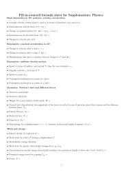
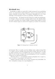
T − V plot. A typical plot is shown in figure 2.1. The change in the temperature
dependence of the volume gives rise to a discontinuity in the expansivity when passing
T g . The heat capacity and other thermodynamical derivatives have equivalent
discontinuities at T g . If the glass is kept below T g the liquid approaches equilibrium,
though it happens slowly, and the volume and other properties are therefore time
dependent; the glass ages. This means that strictly speaking the thermodynamic
derivatives are not strictly well defined in the glass. It also leads to hysteresis in
the system. The hysteresis is seen in the re-heating curve which is also indicated in
figure 2.1.
The relaxation time increases very rapidly in the vicinity of T g ; this means that the
aging processes are very slow already a few degrees below T g . When considered at
times shorter than the relaxation time the glass behaves like a solid in all senses.
It is therefore possible to measure and assign meaningful “apparent” values to the
properties of the glass, including the thermodynamical derivatives (figure 2.1).
V or H
αP or cP
T g
Temperature
T g
Temperature
Figure 2.1: Illustration of the temperature dependence of volume, enthalpy and their
temperature derivatives when passing the glass transition.
The freezing in of the liquid at T g has the consequence that the structure of the
glass is that of the liquid when it fell out of equilibrium at T g . The glass is hence
a disordered solid, and it cannot be distinguished from a liquid from a structural
point of view.
A liquid has a T g that depends on the cooling rate (lower cooling rates give lower T g ).

2.1. The glass transition 9
Cooling at very high rates is called quenching. The glasses formed by quenching have
larger specific volume because their properties are frozen in at a higher temperature
and a corresponding higher volume. The term T g is traditionally used about the
temperature at which the liquid falls out of equilibrium when cooled at standard
experimental rates [Ediger et al., 1996]. This in practice happens at the temperature
where the viscosity is 10 12 Pas ∼ 10 13 Pas and the alpha relaxation time (τ α ) is of
the order 100 s ∼ 1000 s. The criterion τ α = 100 s is often used as a definition of
the glass transition temperature.
The traditional route to glass-formation is to cool the liquid at constant atmospheric
pressure. However, the characteristic alpha relaxation time also increases
when pressure is increased along an isotherm. This leads to a freezing in of the
structural relaxation at a given pressure P g , where the relaxation time has reached
100 s ∼ 1000 s. The effects of pressure and temperature on the viscous slowing down
can be considered jointly by describing the alpha relaxation time as a function of the
two: τ α (P, T). Based on this function it is possible to determine lines of constant
alpha relaxation time in the parameter space defined by pressure and temperature.
We shall refer to lines of constant relaxation time as isochrones and consider the
T g (P) line as a special case of an isochrone.
It has been suggested that the viscous slowing down observed at atmospheric pressure
is due to the decrease of the specific volume which follows from cooling [Cohen
and Turnbull, 1959]. However, measurements of the relaxation time as a function
of temperature and pressure have clearly shown that volume alone does not control
the relaxation time. One way to illustrate this is by showing that the isochrones are
not parallel to the isochores in the T − P diagram.
The other extreme would be a situation where the relaxation time is only temperature
dependent. The simplest model of the temperature dependence would be
an activated behavior, where the viscosity or relaxation time is controlled by some
temperature independent activation energy (E a , measured in units of temperature).
This would lead to an Arrhenius temperature dependence:
η = η p exp
(
Ea
T
)
and
τ = τ 0 exp
(
Ea
T
)
, (2.1.1)
where η p and τ 0 are the high temperature limits of the viscosity and the alpha
relaxation time respectively. Arrhenius behavior is actually (almost) followed by
some systems (see below), but this is not the general case. The dependence on
temperature is usually super-Arrhenius, i.e. stronger than the Arrhenius form. It
is possible to keep the notion of an activated behavior by allowing the activation

10 Slow and fast dynamics
energy in equation 2.1.1 to be temperature dependent. In most cases, it also appears
that this activation energy is density (or pressure) dependent. Such an activation
energy can formally be defined from the equation:
or a similar expression for the viscosity.
( ) E(ρ, T)
τ α (ρ, T) = τ 0 exp , (2.1.2)
T
Within the last ten years there has been a lot of progress in mapping out the temperature
and pressure (or T and density) dependences of the alpha relaxation time
particularly in terms of the temperature and density dependences of E(ρ, T). This
approach is central to the present work. However, before presenting the findings in
this field we shall take a step back and introduce some of the other central concepts
and findings in the field. These latter are originally based on studies performed at
constant atmospheric pressure.
In chapter 3 we return to the temperature and density dependence of the dynamics
and at this point we will commence the central aim of the present thesis, namely
to revisit (discuss and test) results obtained at atmospheric pressure by combining
them with our knowledge of the influence of pressure on the dynamics of glasses and
glass-forming liquids.
2.2 Fragility
The glass transition is, as described above the passage from a thermodynamic
(metastable) equilibrium state to a non-equilibrium state. This transition is a natural
consequence of the fact that the relaxation time of the system surpasses the
timescale on which we are able to perform observations. In our opinion the main
question is therefore not to understand the glass transition itself, but rather to
understand why the relaxation time increases so dramatically when the liquid is
cooled.
While the viscous slowing down is universal, there are still large variations to be
found when comparing the temperature dependences seen in different liquids. The
classification and description of systems according to this difference play a major
role in the attempt to understand the universal features of the slowing down.
The concept of “fragility” [Angell, 1991] has become a standard scheme for characterizing
the temperature dependence of the relaxation time (or viscosity) of a
liquid. Fragility is a measure of how much this temperature dependence deviates

2.2. Fragility 11
from Arrhenius form; characterizing a large departure from Arrhenius behavior as
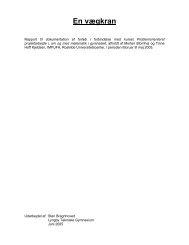
fragile and Arrhenius behavior as strong. This concept of “fragility” is usually illustrated
by a so-called Angell plot (figure 2.2) in which the logarithm of the relaxation
time (or viscosity) is shown as a function of the inverse temperature normalized by
the glass transition temperature. An Arrhenius temperature dependence, that is a
strong behavior (equation 2.1.1), yields a straight line with slope log(τ g /τ 0 ) in this
type of plot, while a fragile behavior corresponds to a concave curve.
Several different measures have been suggested in order to quantify the fragility.
They are essentially equivalent, but they also express slightly different interpretations
of the concept itself.
Figure 2.2: The logarithm of the viscosity as a function of the inverse temperature
normalized by the glass transition temperature. Arrhenius temperature dependence,
that is a strong behavior (equation 2.1.1) yields a straight line with slope log(τ g /τ 0 )
in this type of plot, while a fragile behavior corresponds a concave curve. This type
of plot is often called an Angell plot. The figure is taken from Angell [1991].
The most common measure of fragility is the steepness index, which measures the
low temperature limit of the slope of the curve in the Angell plot [Angell, 1991].
The steepness index is given by
m = dlog 10(τ)
dT g /T (T = T g). (2.2.1)
m equals 16 for strong liquids if it is assume that log 10 τ 0 = −14 and increases with

12 Slow and fast dynamics
increasing fragility, with m ∼ 80 being a typical value for a fragile molecular liquid.
Another possible approach is to fragility is to use master curves, actually fitting
formulae, for the temperature dependence of the relaxation time. The most common
formula is the Vogel-Fulcher-Tammann (VTF) function [Vogel, 1921]
log 10 (τ) = A V F +
B
(T − T 0 )
(2.2.2)
where A V F , B and T 0 are constants. The three constants give (as far as the fit is
good) a characterization of the global temperature dependence and as a result of
the fragility. More specifically, fragility is characterized by a unique dimensionless
parameter D = B/T 0 , a small D characterizing a fragile system and a large one a
strong system (formally when T → 0 one recovers an Arrhenius behavior and D →
∞). A similar characterization has been proposed on the basis of the frustration
limited domain theory, fragility being then measured by a unique dimensionless
parameter related to the frustration strength [Kivelson and Tarjus, 1998]. The
connection between these fragility parameters and the steepness index is found by
differentiation of the expression for the relaxation time: (m = BT g (T g − T 0 ) −2 ) in
the case of equation 2.2.2. The VTF-function is useful for interpolating data over
several decades in relaxation time, but it is rarely found to give a good fit over the
total range from τ 0 to τ g . The fragility so determined will therefore depend quite
strongly on the range of data included when fitting (see also section 5.2).
On the other hand, one can consider the fragility as something that changes with
temperature (or relaxation time). From figure 2.2 it is clear that even the liquids
which become non-Arrhenian at low temperatures have an essentially Arrhenius
temperature dependence at high temperatures. This change in temperature dependence
can hence be considered as a transition from a strong to a fragile domain for
a given liquid.
The steepness index is originally defined at T g but it can in principle be evaluated
at other times, leading to a more general definition, in which the steepness index
becomes relaxation time dependent
m(τ) = dlog 10 τ
dT τ /T
(2.2.3)
where τ(T τ ) = τ defines T τ .
Inserting the Arrhenius temperature dependence (equation 2.1.1) we get the time

2.3. Non-Debye relaxation 13
dependent steepness index of a strong liquid,
m strong (τ) = log 10 (τ/τ 0 ) (2.2.4)
which takes the value m strong (τ = 100s) = 16 (assuming τ 0 = −14) and decreases
to m strong (τ = τ 0 ) = 0 as relaxation time is decreased. The steepness index is
thus relaxation time dependent even for a strong system and the steepness index is
therefore an inconvenient measure of the relaxation time dependent departure from
Arrhenius. A measure more adapted for studying the fragility at different times is
the index introduced by Olsen [Dyre and Olsen, 2004].
dlog E(T)
I(τ) = −
dlog T (T = T τ) (2.2.5)
where E(T) is a temperature dependent activation energy defined by E(T) = T(lnτ−
lnτ 0 ). The Olsen index will take the value 0 at all relaxation times in a system where
the relaxation time has an Arrhenius temperature dependence. Systems with a typical
fragile behavior have I = 0 at high temperatures (short relaxation times) where
they follow an Arrhenius behavior and an increasing I as the temperature dependence
starts departing from Arrhenius. Typical values of I at T g (τ = 100s) are
ranging from I=3 to I=8 corresponding to steepness indices of m=47 to m=127.
There is a one to one relation between the steepness index and the Olsen index
[Dyre, 2006], and one finds that the Olsen index essentially is the relaxation time
dependent steepness index normalized to its value in a strong liquid,
I(τ) =
m(τ)
log 10
(
τ
τ 0
) − 1 =
m(τ) − 1, (2.2.6)
m strong (τ)
where the last equality follows from inserting equation 2.2.4. This type of normalized
fragility measure has also been suggested by Granato [2002].
In this work we mostly use the conventional shorthand of referring to the steepness
index evaluated at T g as the fragility of a given system. We also use the Olsen index,
mainly conceptually, in some situations where it is particularly convenient.
2.3 Non-Debye relaxation
The understanding of the super-Arrhenius temperature dependence of the alpha
relaxation discussed above is maybe the main question in the research field of glassforming
systems. Another key question is to understand the characteristics of the

14 Slow and fast dynamics
(linear) relaxation itself.
Simple Debye (exponential) relaxation is very rarely found in viscous liquids, hence
the relaxation is non-Debye. Instead the relaxation function is found to be broader
than a Debye relaxation. This can either be described as a superposition of Debye
processes or by one of the numerous phenomenological fitting functions which are
used in the area (see section 5.3 for details).
The most general question, concerning non-Debye relaxation in macroscopic quantities,
is whether it is due to an intrinsic non-Debye relaxation or whether the macroscopic
departure from Debye relaxation is due to heterogeneous dynamics. In a
homogeneous relaxation all the relaxation entities have relaxations identical to the
average relaxation. In a heterogeneous scenario every entity behaves differently, and
in this case it is possible that the individual relaxation is Debye. In this case the
non-Debye average relaxation stems from the fact that it is an average. [Richert,
2002]
In the last decade there has been extensive studies, using different experimental
techniques and simulations, of the heterogeneity of viscous liquids. The most common
conclusion is that the liquid is structurally homogeneous but that the dynamics
is heterogenous. This means that different parts of the liquid move in different ways
at a given time. [Richert, 2002]
A stronger deviation of the relaxation functions from an exponential dependence
on time (a more important “stretching”) has been found to correlate with larger
fragility Böhmer et al. [1993]. The reported correlation between the two is one of
the bases of the common belief that both fragility and stretching are signatures of
the cooperativity of the liquid dynamics. We discuss this correlation in chapter 5.
2.4 Energy landscape
The most detailed question we could ask regarding the dynamics of the liquid is of
course the following: Where are all the molecules as a function of time? That is,
we ask the time dependence of 3N coordinates (N being the number of particles).
But these 3N values are of course not accessible (except in computer simulations)
and moreover it is difficult, if not impossible, to interpret such an overwhelming
amount of information. It is, however, very common in glass physics to think and
argue in terms of the potential energy landscape. The energy landscape is a hypersurface
which describes the potential energy of the system as a function of the 3N
configurational coordinates. The dynamics of the liquid is viewed as an exploration

2.5. Fast dynamics and glassy dynamics 15
of this landscape. This view of the liquid dynamics was introduced by Goldstein
[1969] and it has been used extensively in the last decade as a tool in computer
simulations, theoretical work, as well as in the interpretation of experimental results.
In the temperature interval just above T g , it is generally agreed on that the structural
relaxation is dominated by hopping between energy minima, whereas short time
dynamics can be viewed as vibrational modes around the minima. The structural
relaxation and its timescale are thus governed by the typical barrier heights between
the minima (directly related to the notion of the activation energy discussed in the
preceding section), while the vibrations are governed by the shape of the minima.
The characteristic time scales of the vibrations is ∼ 10 −13 s while the alpha relaxation
at temperatures close to T g has a characteristic time of seconds, which means that
there is a tremendous separation between the relevant time scales.
2.5 Fast dynamics and glassy dynamics
The vibrations mentioned above are also present in the glass, after the structural
relaxation has been frozen in. This means that the dynamics of the liquid at short
times is directly related to the dynamics in the glass. However, for the purpose
of later discussions we would like to make a distinction between the fast (or high
frequency) dynamics of the equilibrium liquid and the dynamics in glass.
2.5.1 Fast dynamics in equilibrium
At short times the liquid behaves like a solid in the sense that the particles appear
to be just vibrating around equilibrium positions. At longer times the particles
will start diffusing. The characteristic time defining the transition from solid-like
behavior to liquid-like behavior is the structural (alpha-) relaxation time discussed
in section 2.1. If the alpha relaxation time is very short, as it is the case at high
temperatures in non-viscous liquids, then it is not possible to make this separation
in different dynamic regimes.
Another way of picturing the separation of time scales in viscous liquids is to consider
the response to an external perturbation. If the liquid is subjected to, say
an instantaneous hydrostatic pressure, then it will be compressed by some finite
quantity (quasi) instantaneously. This response is solid-like; it corresponds to the
movements of all the particles against an effective spring constant at their current
position. As time is increased the particles have time to rearrange, the liquid relaxes,
and a new equilibrium is obtained.

16 Slow and fast dynamics
The dynamics with characteristic time shorter than the alpha relaxation time is
what we refer to as fast dynamics or equivalently high frequency dynamics.
Measurements at a fixed frequency or fixed time scale naturally do not probe the
time dependence of the dynamics. What they see is the dynamics on the time scale
they are sensitive to. This means that a measurement with a timescale considerably
shorter than the alpha relaxation time (or a frequency larger than the inverse alpha
relaxation time) only probes the fast dynamics of the viscous liquid.
The fast (linear) dynamics are, like any other property of the (viscous) liquid, dependent
on the thermodynamic state determined by temperature and pressure. This
means that properties characterizing fast dynamics, such as high frequency moduli,
short time mean square displacement, etc. depend (sometimes strongly) on pressure
and temperature. Fast dynamics are sometimes referred to as glassy dynamics
because it is the dynamics at times faster than the structural relaxation, which
governs the glass transition. However, fast dynamics measured in viscous liquids
in their thermodynamic (metastable) equilibrium state are equilibrium properties.
This means that they are not history nor path dependent, but uniquely determined
by the thermodynamic state of the liquid.
2.5.2 Glassy dynamics
The glassy state is, as described in section 2.1, a non-equilibrium state obtained
when the alpha relaxation becomes so long that it is not possible to wait for the
liquid to reach its thermodynamic equilibrium. All dynamical processes happening
on the alpha relaxation time scale are consequently frozen in. However the particles
keep moving in a solid-like manner, hence the fast dynamics stay active, and these
remaining dynamical processes are what we refer to as glassy dynamics. The important
distinction between the fast dynamics in the equilibrium liquid and the glassy
dynamics is that the former is a well defined equilibrium quantity while the latter is
a property of the non-equilibrium glassy state. The properties characterizing glassy
dynamics are therefore in principle path and time dependent, as is characteristic for
properties in non-equilibrium systems.
It turns out that the path and time dependence of the glassy properties is only seen
when the glass is subjected to quite extreme treatments such as very long waiting
times, quenching or compression in the liquid and decompression in the glass. When
the glass is cooled under “normal” isobaric conditions, not much happens under
cooling. When the glass is formed the structure is frozen in, and this has the
phenomenological consequence that most properties have very weak temperature

2.6. Fragility and other properties 17
dependence in the glass. This is also true for the glassy dynamics, which as we
shall see in many cases just correspond to the fast dynamics in the liquid measured
at T g . From the phenomenological point of view it is thus found that the major
difference between glassy dynamics and fast dynamics in the liquid is that the former
is virtually temperature independent while the latter can depend on temperature.
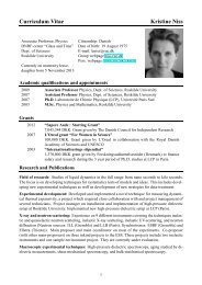
Figure 2.3 illustrates how the glassy dynamics correspond to the fast dynamics.
2.5.3 Time scales - the actual phenomenology
In the above we have considered dynamics happening at two different timescales.
The actual phenomenology of glass-forming liquids is somewhat more complicated
and also system dependent. The structural relaxation often bifurcates in two separate
relaxations when the structural relaxation time is lower than approximately
10 −5 s. The process which appears in addition to the alpha process is faster and it
has lower intensity as well as weaker temperature dependence. It is referred to as
the slow beta-relaxation or the Johari Goldstein (JG) beta relaxation. The position
of the bifurcation point differs by several decades from system to system (and from
one experimental probe to another). Moreover, there are also numerous systems
where this separation in two relaxations is not detectable. The JG-beta relaxation
is faster than the alpha relaxation and it also stays active when the glass is formed.
As such it is part of the fast as well as of the glassy dynamics. We shall deal a bit
with the JG-process when discussing the interpretation of dielectric spectroscopy in
chapter 5. However, the fast dynamics studied and discussed in this work occurs on
a still faster time scale, namely in the pico-nanosecond range.
2.6 Fragility and other properties
The fragility introduced in section 2.2 is the central point in our description of slow
dynamics, and the main problem addressed here is to understand which properties
(if any) relate to the fragility. The ultimate goal is to look for causal relations and
to use them to understand what governs the viscous slowing down.
We have already mentioned in section 2.3 that the fragility has been suggested to
correlate to the departure from Debye relaxation. This correlation is just one among
a large body of properties that have been suggested to correlate to the fragility.
The excess in entropy of the liquid as compared to that of the glass has been found
to decrease faster as a function of decreasing temperature in fragile liquids than

18 Slow and fast dynamics
T > T 2
κ
ω T 2 > T > T 1
1
κ
ω 2
T 1 > T
T 1 T 2
ω 1 ω 2
Figure 2.3: The left figure shows an idealized illustration of the temperature dependence
of the compressibility measured at two different time scales, a high frequency
ω 2 and a low frequency ω 1 (with the latter corresponding to the timescale of the
cooling rate). The right figure shows the corresponding frequency dependent compressibility
at different temperatures. The jump in level is the signature of the
temperature dependent alpha relaxation. The probe frequencies are indicated with
vertical lines. The figure illustrates three domains. At temperatures above T 2 the
two probes measure the same low frequency compressibility - its value decreasing
with decreasing temperature. At temperatures lower than T 2 but higher than T 1 the
high frequency probe measures the high frequency value of the compressibility while
the low frequency probe measures the low frequency value. Both high frequency
and low frequency compressibility depend on temperature, but not a priori with
the same temperature dependence. At temperatures lower than T 1 both probes see
the high frequency compressibility. This is so because the alpha relaxation time
has become longer than the time scale of both probes. The alpha relaxation is also
longer than the characteristic time of cooling - meaning that liquid is frozen in its
glassy state. This freezing in also has the consequence that the measured compressibility
does not change significantly with decreasing temperature. The value of the
compressibility in the glass corresponds to the high frequency compressibility at T g
when the liquid is frozen in.

2.6. Fragility and other properties 19
in strong liquids. This correlation is originally rationalized in terms of the Adam-
Gibbs model [Adam and Gibbs, 1965]. The Adam-Gibbs model is based on the
notion of cooperative dynamics that demand larger and larger cooperative regions
as the temperature is lowered. It is moreover assumed that the activation energy is
proportional to the volume of the rearranging region. The fundamental assumptions
of the model have been questioned several times, but the model continues to play an
important role in the community and it has also re-derived from different starting
points [Kirkpatrick et al., 1989; Bouchaud and Biroli, 2004]. The related idea, that
there is a dynamical length scale in the liquid which grows in the liquid as it is
cooled, is widely believed to play an important role for understanding the viscous
slowing down. The existence of dynamical length scales have been demonstrated
by several techniques [Ediger, 2000; Berthier et al., 2005], but it remains unclear if
they are all interrelated and if the length scale or its evolution with temperature is
related to fragility.
In this work we focus on results which suggest a relation between the viscous slowing
down and other dynamical properties of the liquid or the glass. We particularly
consider four situations, namely: the correlation between fragility and stretching
of the alpha relaxation [Böhmer et al., 1993] in chapter 5, the correlation between
fragility and a smaller ratio of elastic to inelastic signal in the X-ray Brillouin-spectra
[Scopigno et al., 2003] in chapter 6, the correlation between fragility and the short
time mean square displacement, its absolute value [Ngai, 2000] and its temperature
dependence [Dyre and Olsen, 2004; Buchenau and Zorn, 1992] in chapter 7, and
the correlation between fragility and a lower relative intensity of the boson peak
[Sokolov et al., 1993] in chapter 8. Other correlations which might be related but
which we do not treat directly are the correlation between fragility and a larger
Poisson ratio [Novikov and Sokolov, 2004] and the correlation between fragility and
a stronger temperature dependence of the elastic shear modulus, G ∞ , in the viscous
liquid [Dyre, 2006].
The different correlations are in most cases not understood and their validity is often
controversial [Yannopoulos and Papatheodorou, 2000; Yannopoulos et al., 2006 a;
Huang and McKenna, 2001].
The aim is to use these empirical correlations between m P and glassy properties in
testing and developing models and theories of the dynamics in viscous liquids. The
correlations are mostly found empirically as correlations to the fragility measured
under isobaric conditions. In the other hand, the interpretation of the correlations
is always that the property which correlates to fragility is related to the temperature
dependence of the relaxation times. In the same vein computer-simulation as well

20 Slow and fast dynamics
as theoretical attempts to understand these correlations, and fragility in general,
mainly consider isochoric conditions, hence taking only into account the effect of
temperature (e.g. [Parisi et al., 2004; Bordat et al., 2004; Srivastava and Das, 2001;
Ruocco et al., 2004]).
2.7 Relation between fast and slow dynamics
The correlations regarding the stretching, which was introduced in section 2.3, relates
different aspects of the alpha relaxation in the liquid to each other. The three
other correlations, which we shall consider, fall in a category of results in which
glassy or short time dynamics are related to the viscous slowing down. The hypothesis
that there is a relation between fast and slow dynamics is based on striking
empirical results reported in literature over the last decade [Novikov and Sokolov,
2004; Scopigno et al., 2003; Ngai, 2004; Sokolov et al., 1993, 1997; Dyre and Olsen,
2004; Buchenau and Wischnewski, 2004; Buchenau and Zorn, 1992]. A number of
these results (and earlier related results) are reviewed and combined by Dyre [2004,
2006]. Also, Novikov and Sokolov [2004] and Novikov et al. [2005] discuss a variety
of this type of results and suggest that they are intimately connected to each other.
In the following we shortly define the high frequency and glassy properties that have
been suggested to relate to the viscous slowing down. More technical details as well
as discussions of the interpretations are given in chapters 6 to 8 where we study
these properties, and particularly how they depend on pressure.
2.7.1 Nonergodicity factor
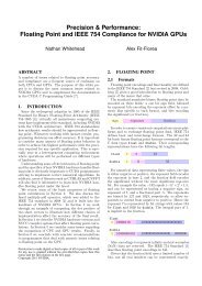
Scopigno et al. [2003] define the nonergodicity factor from the ratio of the central
line intensity over the total intensity of the frequency dependent dynamical structure
factor measured by inelastic X-ray scattering (IXS). The authors look at the
temperature dependence of this quantity in the low temperature limit of the glass
phase and find that the stronger this temperature dependence the more fragile the
liquid (see also section 4.3.7 and chapter 6). This result indicates that a property
measured deep in the glass holds information about the viscous slowing down.
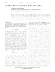
The intensity of the side peaks (figure 2.4) is governed by the characteristics of the
vibrational modes (see section 4.3.7) and as a result by the curvature of the visited
minima of the energy landscape. The correlation therefore suggests that the
shape of the minima is related to other properties of the energy landscape [Scopigno
et al., 2003]. However, it is also possible to take a different view on the correlation

2.7. Relation between fast and slow dynamics 21
S(Q,ω)
−20 −10 0 10 20
ω [meV]
Figure 2.4: Dynamical structure factor measured by inelastic X-ray scattering (IXS).
The nonergodicity factor is defined by the ratio of the central intensity over the total
intensity.
Figure 2.5: Correlation between fragility and the parameter α [Scopigno et al.,
2003]. α is a measure of the temperature dependence of the nonergodicity factor.
See section 6.4.1.

22 Slow and fast dynamics
and suggest that it is related to the intensity of the central peak [Buchenau and
Wischnewski, 2004]. The central peak is a measure of the density fluctuation that
are frozen in when the alpha relaxation is arrested at the glass transition. Hence,
this view on the correlation points to a relation between the amplitude of the alpha
relaxation at T g and the temperature dependence of the alpha relaxation.
2.7.2 Mean squared displacement
The mean squared displacement is classically proportional to temperature in the
harmonic approximation, where the shear and bulk moduli are constant. This linear
behavior is often followed in the glass, but the temperature dependence of the short
time mean squared displacement becomes stronger at temperatures above T g (see
figure 2.6). Moreover, the temperature dependence of the mean square displacement
above T g has been found to be stronger the more fragile the system is [Ngai, 2004].
In this situation it is therefore the high frequency (and not the glassy) dynamics
of the equilibrium liquid that is related to fragility. Some of the interpretations of
the finding are however very close to some of the notions suggested to understand
the above result concerning the nonergodicity factor: namely, that the shape of the
minima in the energy landscape are related to the energy barriers. In this view
it is assumed that the vibrations stay essentially harmonic above T g but that the
curvature of the potential around the minima visited by the system changes as a
function of temperature once the alpha relaxation becomes active. The change of
curvature is expected to also change the barrier height and thereby the temperature
dependence of the alpha relaxation time itself [Dyre and Olsen, 2004].
Another interpretation of the change in the temperature dependence of the mean
square displacement is that it is related to the setting in of fast relaxational processes
[Buchenau and Zorn, 1992; Ngai, 2000]. These processes are thought to serve as
precursors of the alpha relaxation, with the alpha relaxation being faster the larger
the amplitude of these relaxations.
There is in both views a subtle suggestion of a two way causality. A larger amplitude
of the mean square displacement gives rise to a faster alpha relaxation, and the alpha
relaxation itself changes the liquid structure and thereby changes the properties
which govern the mean square displacement.

2.7. Relation between fast and slow dynamics 23
Figure 2.6: The mean square displacement of selenium as a function of temperature.
It is clearly seen that there is a qualitative change in behavior at T g . The authors find
that the temperature dependence of 〈u 2 〉 loc (indicated in the figure) is proportional
to the temperature dependence of the logarithm of the alpha relaxation time, ln(τ α ).
[Buchenau and Zorn, 1992]
2.7.3 Boson Peak
The low energy (

24 Slow and fast dynamics
The boson peak modes have an energy corresponding to the plane waves with
nanometer wavelength. This leads to the expectation that it is the disorder on
this length scale which will be determining for the boson peak. Similar length scales
are often associated with the cooperative dynamics of the alpha relaxation close to
the glass transition. [Leonforte et al., 2006]
2
DBF and Bose Scaled S(ω)
1.5
1
0.5
I max
I min
R=I min
/I max
ω / meV
0
0 5 10 15
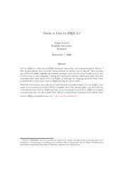
Figure 2.7: Incoherent dynamical structure factor measured by inelastic neutrons
scattering (INS). It is illustrated of how to determine the ratio R which gives a
measure of the relative boson peak intensity.
The most direct relation suggested between the boson peak in the glass and the slow
dynamics in the liquid is the correlation between the relative boson peak intensity
and fragility proposed by [Sokolov et al., 1993, 1997] (see figures 2.7 and 2.8). It is
speculated that this correlation means that strong systems have a larger degree of
disorder than the fragile ones when the system is frozen in and the glass is formed
[Novikov et al., 2005].
Figure 2.8: Correlation between m P and relative boson peak intensity. The left
figure shows the inverse boson peak intensity in terms of its amplitude over the
Debye density of states g(ω)/g D (ω), the right figure shows the parameter R found
as illustrated in figure 2.7. Both figures are from [Novikov et al., 2005].

2.7. Relation between fast and slow dynamics 25
2.7.4 Other results
We shall shortly discuss two other results relating fast or glassy dynamics to the
alpha relaxation. These results are not discussed nor tested in detail in this work,
but are included here for completeness and because they have been suggested to
relate to the results discussed above. Both these results concern the high frequency
shear modulus of the liquid.
The shear modulus of a liquid goes to zero in the high temperature or low frequency
limit while the bulk modulus is non-zero under all conditions. This means that
longitudinal sound waves always are present in liquids, whereas shear modes exist
only at low temperatures or short times, such that the probe frequency is faster
than the alpha relaxation time τ α > 1/ω probe . The non-zero shear modulus is thus
a signature of being in a domain where the structural relaxation is frozen.
Shoving model
The shoving model [Dyre et al., 1996] suggests that it is the high frequency shear
modulus which controls the activation energy (equation 2.1.2). The rationale for
suggesting that a high frequency property governs the alpha relaxation is that while
the alpha relaxation is slow, the actual rearrangements (the hops in the energy
landscape) happen on a short time scale. The choice of the shear modulus stems from
a macroscopic elasticity theory calculation in which it is assumed that a local volume
expansion is needed for the rearrangement to be possible. Such an expansion will in
the simplest case of a spherical geometry be governed by the shear modulus. The
shoving model is in one approximation 2 equivalent to a model where the activation
energy is proportional to temperature over mean square displacement, E(ρ, T) ∝
T/〈u 2 〉. We follow Dyre [2006] and refer to the model in this form as the elastic
model. We discus the elastic model in our study of the mean square displacement
in chapter 7.
Poisson ratio
Novikov and Sokolov [2004] found from comparing about a dozen different glass formers
that there is a correlation between fragility and the ratio of the bulk to the shear
2 The equivalence follows from the fact that the shear modulus dominates over bulk modulus in
determining the temperature dependence of the mean square displacement, see [Dyre and Olsen,
2004] for details.

26 Slow and fast dynamics
modulus 3 K/G, meaning that a glass corresponding to a fragile liquid sustains bulk
deformation better than shear deformation. The glassy moduli correspond to the
high frequency moduli of the liquid at the glass transition (see section 2.5) and the
correlation can therefore be expressed as a correlation to the ratio K ∞ /G ∞ between
the high frequency moduli in the liquid at T g [Novikov et al., 2005]. The authors
moreover suggest that this correlation is directly related to the correlation suggested
by Scopigno et al. [2003]. The argument is based on assuming that difference between
high frequency and low frequency bulk moduli is much smaller than the high
frequency shear modulus, K ∞ − K 0 ≪ G ∞ . However, this assumption is not found
to hold [Scopigno, 2007], rather the two are of similar size (e.g. [Barlow et al., 1969;
Christensen, 1994]). Lastly, it is worth mentioning that the correlation has been
tested on a much larger set of glass-formers by Yannopoulos and Johari [2006] and
Johari [2006], who demonstrated that different types of glass formers have different
behaviors. The correlation does however seem to hold when comparing systems of
the same class of glass-formers.
3 The ratio K/G is larger the larger is the Poisson ratio σ = 3K/2G−1
3K/2G+1
, so this correlation implies
a correlation between fragility and the Poisson ratio.

Résumeé du chapitre 3
Traditionnellement on forme un verre par refroidissement à pression atmosphérique,
c’est à dire dans des conditions isobares. Le refroidissement isobare a deux effets
simultanés sur le liquide : l’énergie thermique diminue et la densité augmente. La
possibilité de former un verre soit par refroidissement isochore soit par compression
isotherme montre bien que ces deux effets contribuent tous deux au ralentissement
visqueux. Pour mieux comprendre le ralentissement visqueux et la transition vitreuse,
il est donc important de pouvoir séparer l’effet de l’énergie thermique et l’effet
de la densité. Ce type de séparation est uniquement possible si on a accès aux temps
de relaxation (ou aux viscosités) et aux données PVT pour un même système. Durant
les dix dernières années, de nombreuses études sur ce sujet ont permis d’aboutir
à l’existence d’une loi d’échelle universelle.
Dans le premier paragraphe de ce chapitre, on introduit le formalisme nécessaire
à la description de la dépendance en température et en densité du temps de relaxation.
Le deuxième paragraphe résume l’émergence de cette loi d’échelle et ses
conséquences.
Les corrélations proposées dans la littérature entre les caractéristiques dynamiques
d’un liquide vitrifiable et sa fragilité ont toujours été proposées sur la base de données
expérimentales mesurées à pression atmosphérique. Le but principal de cette thèse
est de tester si les corrélations sont robustes en pression et d’utiliser la séparation
entre effet de température et effet de densité pour mieux comprendre le sens physique
de ces corrélations. Dans le dernier paragraphe de ce chapitre, on développe des
arguments généraux dens ce sens, qui seront utiles dans les quatre chapitres suivants.

Chapter 3
What we learn from pressure
experiments
In this chapter we first introduce earlier results on density and pressure dependence
of the alpha relaxation (section 3.1 and 3.2) and next develope a framework in order
to better understand different types of correlations with fragility (section 3.3 and
3.4).
The steepness index is mostly used as a measure of fragility, but the results and
arguments, hold for other types of fragility criteria, e.g. the Olsen index just as
well.
3.1 Isochoric and isobaric fragility
The measures of fragility which we introduce in section 2.2 are in their original form
(implicitly) defined at constant atmospheric pressure because this is where most
experiments are performed. For instance the steepness index is actually
m P = ∂ log 10(τ)
∂ T τ /T
∣ (T = T τ ) (3.1.1)
P
where the derivative is to be evaluated at T τ . T τ is defined as being the temperature
at which the relaxation time reaches the value τ, e.g. τ = 100 s. The conventional
fragility is hence the atmospheric pressure isobaric fragility. However, the relaxation
time can also be measured as a function of temperature along other isobars. This
is illustrated in figure 3.1 where it can also be seen that the T τ (P) increases when
pressure increases. Isobaric fragility is well defined at any point on the isochronic
29

30 What we learn from pressure experiments
T τ -line and isobaric fragility evaluated at a given relaxation time can be considered
as a function of pressure. Empirically, it is most often found that isobaric
fragility decreases with pressure, but it can also be increasing or virtually pressure
independent [Roland et al., 2005].
In addition to the isobaric fragility, it is also possible to define an isochoric fragility:
m ρ = ∂ log 10(τ)
∂ T τ /T
∣ (T = T τ ). (3.1.2)
ρ
The isochoric fragility is a measure of how much the temperature dependence of
the relaxation time departs from Arrhenius when the liquid is subjected to isochoric
cooling. Isochoric cooling is often performed in simulations which makes this
distinction particularly important when comparing experimental and simulation results.
Experimentally, it is difficult to perform isochoric cooling, but the isochoric
derivative is nonetheless a well defined quantity.
The two fragilities are straightforwardly related by the chain rule of differentiation:
m P = ∂ log 10(τ)
∂ T τ /T
= m ρ + ∂ log 10(τ)
∂ρ
∣ (T = T τ ) + ∂ log 10(τ)
∂ρ
ρ
∂ρ ∣
T
∂ T τ /T ∣ (T = T τ ) (3.1.3)
P ∣
∂ρ
∂ T τ /T ∣ (T = T τ ) (3.1.4)
P
∣
T
when both are evaluated at the same thermodynamic state point, e.g. at a given
pressure P 1 defining (T τ (P 1 ), ρ(P 1 , T τ (P 1 ))). Expressed in this way the effects leading
to the slowing down when cooling along an isobar is separated in two contributions:
(i) the slowing down due to the decrease of temperature itself, and (ii) the contribution
from the increase of density which follows as a consequence of decreasing
temperature [Ferrer et al., 1998].
Equation 3.1.3 can be rewritten to
m P = m ρ (1 − α P /α τ ) (3.1.5)
where α P is the isobaric expansivity α P = −1 ∂ρ
ρ ∂T
∣ while α τ = −1 ∂ρ
P
ρ ∂T
∣ is the
τ
isochronic expansivity; that is a measure of volume changes as a function of temperature
along an isochrone (a line where the alpha relaxation time is constant) [Ferrer
et al., 1998]. We want to stress that equation 3.1.5 is exact. It only builds on the
definitions introduced and some standard differential algebra 1 .
1 The equivalence between equation 3.1.3 and 3.1.5 can be shown from the relation
˛ ∂T τ /T ˛ ∂ρ
∂ρ ∂log τ
˛˛˛T=-1.
∂ log 10 (τ)
∂ T τ /T
˛ρ
˛τ

3.2. Empirical scaling law and some consequences 31
Equation 3.1.5 shows that the difference between m P and m ρ is determined by the
ratio of two expansivities, α τ and α P . However, the difference is not determined
by thermodynamics alone because α τ contains dynamical information as well, since
it is necessary to know the slope of the isochrone (e.g. the glass transition line) in
order to evaluate it.
Turning now to the phenomenology, it is well known that α P is positive 2 ; α τ on the
other hand is negative because density increases as with increasing temperature when
moving along an isochrone (see figure 3.1 a). By inserting these simple empirical
facts in equation 3.1.5 can be seen that the isobaric fragility is larger than the
isochoric fragility.
3.2 Empirical scaling law and some consequences
Within the last decade a substantial amount of relaxation time and viscosity data
has been collected at different temperatures and pressures/densities, mainly by the
use of dielectric spectroscopy. On the basis of the existing data it is relatively well
established that the temperature and density dependence of the relaxation times
can be expressed as first suggested by Alba-Simionesco et al. [2002], as
( ) e(ρ)
τ(ρ, T) = F . (3.2.1)
T
The result is empirical and has been supported by the work of several groups for a
variety of glass-forming liquids and polymers [Alba-Simionesco et al., 2002; Tarjus
et al., 2004 a; Casalini and Roland, 2004; Roland et al., 2005; Dreyfus et al., 2004;
Reiser et al., 2005; Floudas et al., 2006]. See also chapter 5 in this work.
3.2.1 The result and its history
The scaling can also be expressed in terms of the activation energy defined in equation
2.1.2. In fact is was first proposed in its general form from the idea of reducing
the influence of density on the slowing down to a single density dependent activation
energy scale [Alba-Simionesco et al., 2002; Alba-Simionesco and Tarjus, 2006]:
( )
E(ρ, T) T
E ∞ (ρ) = Φ . (3.2.2)
E ∞ (ρ)
2 Except for tetrahedral systems at certain temperatures, eg. water below 4 ◦ C.

32 What we learn from pressure experiments
2
log 10 (τ)
P2 >
P atm
m P (P2)
P atm
Pressure
Glass transition line
Isochores
glass
liquid
P2
ρ 1
ρ 2
log 10 (τ)[s] log 10 (τ)[s]
-10
2
-10
log 10 (τ)
1/T
T g (P)/T
ρ2 > ρ1
ρ1
1/T
m P (P atm)
isobars
1
m ρ
isochors
a) Temperature
Patm
b) T g (ρ)/T
1
Figure 3.1: Typical PVT diagram for a glass-forming liquid. The glass transition
line is the line where the structural relaxation time reaches τ = 100s; the glass
transition line is thus a specific example of an isochrone. The system is out of
thermodynamical equilibrium on the left hand side of the glass transition line and the
density is therefore path dependent. The thin dashed-dotted lines indicate typical
glassy isochores corresponding to a density obtained by cooling isobarically after
crossing the T g line. The thin dashed lines illustrate two isochoric cooling paths in
the liquid, while the bold dashed lines illustrate two isobaric cooling paths (P atm
and P2 > P atm ). b) top: typical temperature dependence of the relaxation time
when followed at different isobars. It is illustrated that this temperature dependence
persists after scaling with T g (P) leading to a pressure dependence in m P . The open
symbols correspond to the highest pressure (P2). b) bottom: typical temperature
dependence of the relaxation time when followed along different isochores. The
density dependence is canceled by scaling with T g (ρ) which means that m ρ is density
independent. The open symbols correspond to the highest density (ρ2 > ρ1).

3.2. Empirical scaling law and some consequences 33
The index ∞ refers to “T → ∞” because Alba-Simionesco et al. [2002] associate
E ∞ (ρ) with the activation energy in the high-temperature liquid regime where the
relaxation time has an Arrhenius temperature dependence.
Prior to this, partial results indicative, or compatible with, the above expression
had been found. For instance, Tölle [2001] had shown that the relaxation time in
liquid oTP at the nanosecond time scale measured at different pressures could be
superimposed when comparing sets of temperature and pressure that correspond to
the same value of Γ = ρT −1/4 . This was motivated by the model of soft spheres
in which the liquid is described by a single control parameter Γ = ρT −3/n , with
n being the exponent of the repulsive pair potential r −n [Hansen and McDonald,
1986]. Dreyfus et al. [2003] extended this finding for oTP in the viscous regime with
relaxation times obtained from light scattering data.
The formulation by Tölle can be recast in the form proposed by Alba-Simionesco
et al. [2002] if the density dependence of E ∞ (ρ) is a power-law with exponent 4 as
first demonstrated by Tarjus et al. [2004 a]. This can be seen from inserting equation
3.2.2 in equation 2.1.2 (τ(ρ, T) = τ 0 exp(E(ρ, T)/T)):
(
E∞ (ρ)
τ(ρ, T) = τ 0 exp
T
τ(ρ, T) = F 1
(
E∞ (ρ)
T
( )) T
Φ
E ∞ (ρ)
(3.2.3)
)
, (3.2.4)
which is equivalent to equation 3.2.1 and further inserting a power-law E ∞ (ρ) = Cρ x
( )
τ(ρ, T) = F 1 C ρx ( ρ
)
= F 2
T T 1/x . (3.2.5)
where F 1 is a system specific scaling function and F 1 (X) = F 2 (X 1/x ).
[Chauty-Cailliaux, 2003] [Alba-Simionesco et al., 2004] checked the above scaling on
the dielectric data of several glass-forming polymers. In such system for which one
does not have access to the high-temperature regime, hence to E ∞ (ρ), they used
different simple functional form for describing the density dependence of E ∞ (ρ) or
e(ρ) (see equation 3.2.1), a linear and a power-law dependence, finding a similar
quality of data collapse with the two functions. Casalini and Roland [2004] tested
the power-law scaling on dielectric spectroscopy data in a number of different systems
and found it to work provided the exponent 4 specific to oTP was allowed to become
material dependent. They found it to vary from 0.13 for sorbitol up to more than
8. Dreyfus et al. [2004] did a similar compilation including also light scattering
data. The scaling has since been tested on numerous systems (around 40) by several

34 What we learn from pressure experiments
different groups [Roland et al., 2005; Reiser et al., 2005; Floudas et al., 2006]. The
power law dependence is fulfilled to a good approximation for many systems, but
the range in density is often too small to distinguish from other functional forms
[Dreyfus et al., 2004]. For DBP which we study in this work (chapter 5), we find
significant deviations from the power-law form.
There are some differences in views regarding the physical interpretation of the
scaling law, particularly regarding the meaning of the exponent x Tarjus et al. [2004
a,b]; Roland and Casalini [2004]. In this work we do not deal with the explanation
of the scaling but rather consider its consequences when interpreting other results.
It is therefore important to stress that, despite the controversies, there is agreement
on the phenomenology, so far as to say that equation 3.2.1 gives a good description
of the density and temperature dependences of the relaxation time.
If the density dependent energy E ∞ (ρ) is determined from the high temperature
Arrhenius behavior, then it is given in absolute units - and it is associated with a
specific physical interpretation. However, most of the data leading to the scaling
is obtained in the low temperature non-Arrhenius regime, and the energy is only
obtained up to a multiplicative constant. We have therefore chosen the notation
e(ρ) rather than E ∞ (ρ).
Most of the data supporting the scaling-law is from dielectric measurements in the 0.1
Hz-MHz range. Another limitation of the result is that all the data are on molecular
liquids, Van der Waals bonded or hydrogen bonded or on polymers. Hence, strong
glasses and inorganic glasses in general have not been studied so far. Nevertheless,
the scaling law serves as a general description of the density and the temperature
dependences of the alpha relaxation time in molecular liquids and polymers in the
viscous regime where the super-Arrhenius behavior is seen. Note that if strong
glasses have a strictly Arrhenius behavior, then equations 3.2.1 and 3.2.2 trivially
apply with probably a weak or negligible dependence on density at least for moderate
pressures.
3.2.2 The consequences on fragility
It can be seen directly from equation 3.2.1 that X(ρ, T) = e(ρ)/T, evaluated at
T τ (ρ) has the same value at all densities (X τ = e(ρ)/T τ (ρ)) if T τ (ρ) is defined
as the temperature where the relaxation time has a given value (e.g. τ = 100s).
Exploiting this fact, it is easy to show [Tarjus et al., 2004 a; Alba-Simionesco and
Tarjus, 2006] that the scaling law has the consequence that the isochoric fragility
will be independent of density when evaluated at a T τ corresponding to a given

3.2. Empirical scaling law and some consequences 35
relaxation time:
m ρ = dlog 10(τ)
dT τ /T
∣ (T = T τ ) = F ′ dX
(X τ )
ρ
dT τ /T (T = T τ) = X τ F ′ (X τ ). (3.2.6)
The physical meaning is that temperature T τ changes as a function of pressure, but
the relaxation as a function of temperature will have the same degree of departure
from Arrhenius along different isochores. We illustrate this situation in figure 3.1.
The fact that the relaxation time τ is constant when X is constant means that the
isochronic expansion coefficient α τ is equal ) to the)
expansion coefficient at constant
)
X. Using this and the general result
= −1, it follows that
(
∂ρ
∂T
which inserted in equation 3.1.5 leads to
X
(
∂X
∂ρ
T
( ∂T
∂X
1 dlog e(ρ)
= −T
α τ dlog ρ , (3.2.7)
(
)
dlog e(ρ)
m P = m ρ 1 + α P T τ , (3.2.8)
dlog ρ
where m P and m ρ are again evaluated at a given relaxation time τ.
ρ
This expression illustrates that the relative effect of density on the slowing down
upon isobaric cooling, i.e., the second term in the parentheses, can be decomposed
into two parts: the temperature dependence of the density measured by T τ α P =
− ∂ log ρ
∣ (T = T τ ) , and the density dependence of the activation energy, which is
P
∂ log T
contained in
dlog e(ρ)
d log ρ .
Since m ρ is constant along an isochrone, it follows from equations 3.1.5 and 3.2.8
that the change in m P with increasing pressure is due to the change in α P /α τ =
α P T τ
dlog e(ρ)
d log ρ .
T τ increases with pressure, α P T τ (P) decreases, whereas
dlog e(ρ)
dlog ρ
= x is often to
a good approximation constant in the range of densities accessible 3 . The most
common behavior seen from the data compiled by Roland et al. [2005] is that the
isobaric fragility decreases or stays constant with pressure, with few exceptions. This
indicates that the decrease of α P T g (P) usually dominates over the other factors.
3 The DBP case at high density discussed in section 5.2.1 is one exception.

36 What we learn from pressure experiments
3.3 Correlations with fragility
As described in section 2.6 there is a flourishing variety of correlations between
fragility and other properties of the liquids or its corresponding glass. These correlations
hold a lot of empirical information which should be useful as guidelines and
tests in the development of models and theories of the dynamics in viscous liquids.
However in order for this to be possible, it is important to clarify if the correlations
result from, and consequently unveil information on, the effect of density on
the relaxation time, the intrinsic effect of temperature on the relaxation time, (or
a balanced combination of the two). In the following we provide a framework for
analyzing correlations between fragility and other properties of the liquid or glass
by disentangling temperature and density effects [Niss and Alba-Simionesco, 2006;
Niss et al., 2007]. The arguments presented in this section are not relevant for correlations
between fragility and the temperature dependence in the liquid of some other
property. These types of correlations are specifically considered in section 3.4
3.3.1 Pressure and isobaric fragility
The correlations between fragility and other properties that have been suggested in
literature all refer to the standard isobaric fragility. They are obtained empirically
by plotting the property in question as a function of fragility (measured at T g , τ ≈
100 s -1000 s). The plots obtained in this way are mostly very scattered, which is
to be expected, because specific characteristics of the system can affect either the
fragility or the property which is suggested to correlate with fragility.
Assuming that there is nothing special about atmospheric pressure (from the point
of view of the liquid), then a strict correlation to m P should follow this pressure
dependence, where the property correlating to m P is to be evaluated at the same
pressure. Consequently, the simplest way in which pressure can be used to test
this type of correlation is to view pressure as a smooth way to change the isobaric
fragility without changing the chemistry of the system. The correlation between
isobaric fragility and some chosen property can then be scrutinized by measuring
both quantities as a function of pressure.
If the property in question has a pressure dependence which is consistent with the
correlation then the situation would be the one illustrated in figure 3.2. This type
of agreement would suggest that the property in question is sensitive to the same
factors as the isobaric fragility, m P .

3.3. Correlations with fragility 37
Property
increasing P
Fragility
Figure 3.2: An illustration of how a correlation between a property and isobaric
fragility could be most simply tested with pressure experiments (section 3.3.1).
3.3.2 Isochoric fragility
The existence of a correlation with fragility is always interpreted as indicating that
the property in question is related to the effect of temperature on the structural
relaxation. Moreover, computer simulations and theoretical attempts to understand
these correlations, and viscous slowing down in general, mainly consider isochoric
conditions, hence taking into account only the effect of temperature, see e.g. [Parisi
et al., 2004; Bordat et al., 2004; Srivastava and Das, 2001; Ruocco et al., 2004].
However, when a liquid is cooled isobarically the thermal energy decreases and the
density increases at the same time and the isobaric fragility contains, as we have
seen, information on both these effects.
According to the discussion in section 3.2.2, a property which is related to the pure
effect of temperature should be correlated to the isochoric fragility. From equation
3.2.8 it can be seen that m P contains m ρ , and it has consistently been found by
including a large amount of fragile and intermediate systems that m ρ correlates to
the ambient pressure m P [Casalini and Roland, 2005 a]. It is therefore very possible
that the correlations which have been proposed as correlations to the conventional
isobaric fragility are in fact reminiscences of a more fundamental correlation to m ρ .
The scaling described equation 3.2.1 must be taken as an empirical result and despite
the variety of systems for which it has been shown to hold, there is no guarantee
that it is universal. However, the scaling gives a rationalized picture of the pressure
and temperature dependence of the relaxation time in the data obtained so far on
polymers and molecular liquids. The emerging picture is that m ρ is intrinsic to the
system in the sense that it is density independent. A quantity correlating to the

38 What we learn from pressure experiments
pure temperature dependence of the relaxation time as it is measured by m ρ should
then possess the same intrinsic characteristic and be independent of pressure along
the T g -line. This means that the pressure dependence of a property can help clarify
if it is fundamentally correlated to the intrinsic effect of temperature as measured by
m ρ or rather to the pressure dependent combined effect of density and temperature
as measured by m P .
3.3.3 The relative effect of density
In section 3.3.1 we have considered the pressure dependence of a correlation between
a given property and the isobaric fragility without taking the consequences of the
scaling law into account. If we now incorporate the scaling it follows that m ρ is
density independent and that the pressure dependence of m P (P) is due to a pressure
dependence of α P /α τ (equation 3.1.3). This term is a measure of the relative effect
of density on the viscous slowing down. This underlines that if a correlation follows
the pressure dependence of m P then it is because the property in question is not
just related to the effect of temperature but also to the relative effect of density on
the viscous slowing down.
A last situation which should also be considered is that the correlations suggested
between m P and other properties could in fact be a reflection of the effect of density
on the relaxation time. That is they could fundamentally be correlations to α P /α τ .
In general it is found, as mentioned above, that m ρ is the dominating term governing
m P , which makes such a proposition appear unlikely. However, some of the most
archetypal glass formers, glycerol, salol and oTP who cover a range of m P ≈ 50
to m P ≈ 80, have a very similar isochoric fragility ranging only from m ρ ≈ 38
to m ρ ≈ 45 (see appendix B). Hence, the difference in isobaric fragility found
at atmospheric pressure when comparing these three liquids is not related to an
intrinsically different response to temperature but rather to a different effect of the
change in density upon isobaric cooling (just as it is the case for the change of m P (P)
when changing pressure). If a property is related to the relative effect of density on
the viscous slowing down, then it is expected to correlate with the ratio α P /α τ . This
implies that the property in question should also follow the pressure dependence of
α P /α τ , and as a consequence usually decrease with increasing pressure.
3.3.4 How to evaluate pressure dependence in the glass ?
The properties that are correlated to fragility are often considered at T g . This is for
example true for the stretching parameter β KWW and for the boson peak intensity

3.4. Temperature dependences 39
measured in terms of the parameter R (see figure 2.7). The liquid is at (metastable)
equilibrium at T g and the quantity measured is thus a unique function of the state
point. The fragilities m P and m ρ as well as the ratio α P /α τ are likewise uniquely
defined at these state points. The comparison of the pressure dependence of a
property and the fragilities is therefore naturally done by monitoring the relevant
quantities along the glass transition line T g (P).
The situation is slightly more difficult when the considering a correlation between
fragility and a property in the glass, because the glassy properties under pressure
are path dependent [Chauty-Cailliaux, 2003]. We propose that the relevant path is
the one followed by compressing in the equilibrium liquid and subsequently forming
the glass by cooling. The glass formed in this way has a history equivalent to the
glass formed at atmospheric pressure and the structure in which it is frozen is that
corresponding to the equilibrium liquid at the same pressure. Secondly, one could
in principle distinguish isobaric and isochoric cooling in the glass itself. However,
the expansion coefficient in the glassy state is very small so that this difference can
probably be ignored at least insofar as the dynamics appear to be harmonic.
3.3.5 Temperature dependence of a correlation
In the above we have focused on the pressure dependence of fragility and we have
suggested that a correlation to fragility should be expected also to hold under pressure.
A related question is the relation between dependence on the relaxation time
(or equivalently on temperature) of the chosen property and of the fragility. Should
a property correlated to fragility at T g also be expected to have the same evolution
as the fragility when temperature is raised? And what is the relevant high
temperature-limit in the regime where the liquid follows the Arrhenius behavior?
These questions are hardly meaningful if the property correlated to fragility is a
glassy property. On the other hand they are relevant questions for a property in
the liquid which correlates to fragility. In deed T g is an arbitrary point and if a
correlation is reported at T g it should also be valid at other temperatures, at least
when the liquid stays viscous and equilibrated. Extrapolation of the correlation to
high temperatures and microscopic times may however be meaningless.
3.4 Temperature dependences
The fragility is sometimes suggested to correlate to the temperature dependence of
another property in the liquid. In other words this means that the temperature

40 What we learn from pressure experiments
dependence of the alpha relaxation is suggested to relate to the temperature dependence
of some other property. These types of correlations are typically based
on simple models, e.g. the Adam Gibbs entropy model and the shoving model, but
there are also purely empirical results of this type. Correlations between temperature
dependence of a given property and fragility are somewhat different from the
correlations discussed above. This is because the temperature dependence of a given
property can also be considered both along isochoric paths and along isobaric paths.
The natural expectation is then that the isobaric temperature dependence should
relate to the isobaric fragility whereas the isochoric temperature dependence should
relate to the isochoric fragility. For this scenario to be consistent one hence expects
that the isochoric temperature dependence of the property in question should be
the same along different isochores, corresponding to the fact that isochoric fragility
is density independent.
We now specifically consider the case where the correlation is based on a model in
which the alpha relaxation is considered to be activated with a temperature and
density dependent activation energy which is governed by the property in question,
namely
( ) E(ρ, T)
E(ρ, T) ∝ G(ρ, T) with τ = τ 0 exp . (3.4.1)
T
where G(ρ, T) is the property suggested to govern the activation energy, for instance
the high frequency shear modulus or the inverse configurational entropy.
The first observation is that such models predict that
G(ρ, T)
T
= constant along an isochrone, (3.4.2)
with the isochrone being T g (P) or any other line of constant alpha relaxation time.
Secondly, it follows that there is a direct relation between the temperature dependence
of G and the fragility. In terms of the Olsen index, this can be expressed
as
dlog G
dlog T
∣ (T = T τ ) = I P (τ) and dlog G
P
dlog T ∣ (T = T τ ) = I ρ (τ). (3.4.3)
ρ
The prediction holds at any given relaxation time and for isobaric and isochoric
conditions alike.
The predictions presented so far (equation 3.4.2 and 3.4.3) are direct consequences
of equation 3.4.1 without any further assumptions. If we now make the additional

3.5. Summary 41
assumption that the empirical scaling law (equation 3.2.1) holds, it moreover follows
that the temperature and density dependence of G should be described in terms of
an equivalent scaling law. This is most easily seen by inserting equation 3.4.1 in
equation 3.2.2 (where Φ ′ below is proportional to Φ) :
( ) T
G(ρ, T) = e(ρ)Φ ′ e(ρ)
(3.4.4)
where e(ρ) is the same as in (equation 3.2.1). See also [Alba-Simionesco and Tarjus,
2006] for similar ideas.
3.5 Summary
Fragility involves a variation with temperature that a priori depends on the thermodynamic
path chosen, namely constant pressure (isobaric) versus constant density
(isochoric) conditions. On the other hand, many quantities that have been correlated
to fragility only depend on the thermodynamic state at which they are considered.
It has been found empirically that the isochoric fragility is intrinsic in the sense that
it is independent of pressure when evaluated along an isochrone. Based on these
observation we conclude that a property which is related to the “pure” effect of
temperature on the relaxation time, should correlate to the isochoric fragility (when
comparing systems), and that it should possess the same type of intrinsic character;
that is, they should be constant along an isochrone for a given system. Properties
related to a combined effect of temperature and density are on the other hand expected
to correlate with isobaric fragility and to have a pressure dependence that
corresponds to its pressure dependence - that is most often decrease with increasing
pressure. The ideas put forward in this chapter are a central part of the work and
serve as a reference point for a large part of the analysis in the proceeding chapters.

Résumé du chapitre 4
Au cours de ce travail, on a étudié la dynamique des liquides vitrifiables et des
verres par trois méthodes expérimentales : la spectroscopie diélectrique, la diffusion
inélastique de neutrons et la diffusion inélastique de rayons X. Les principes de base
de ces trois techniques sont présentés dans ce chapitre.
La spectroscopie diélectrique repose sur la mesure de la polarisation d’un échantillon
lorsqu’il est soumis à un champ électrique. On mesure la fonction de réponse, qui
est le rapport entre le champ électrique et la polarisation de l’échantillon. Les
expériences effectuées au cours de cette thèse ont été réalisées en fréquence. Le
champ électrique appliqué est alors sinusoïdal et la réponse est mesurée en fonction
de la fréquence.
La diffusion inélastique repose sur l’interaction entre un faisceau incident, d’énergie
et de vecteur d’onde bien définis, et l’échantillon. On mesure ensuite les modifications
de l’énergie et du vecteur d’onde, qui dépendent des caractéristiques de
l’échantillon. Si on travaille en diffusion neutronique incohérente, on a principalement
accès au facteur de structure incohérent, donc à la fonction d’auto-corrélation.
Lors des expériences de diffusion inélastique de rayons X, on mesure en revanche, le
facteur de structure cohérent, et on sonde donc la dynamique collective de l’échantillon.

Chapter 4
Experimental techniques and
observables
We have so far discussed dynamics in rather loose terms as the relaxations and
vibrations taking place in the liquid. This notion will be precised in this chapter,
where we introduce the dynamical variables we have studied, namely the dielectric
response function and the dynamical structure factor. In this chapter we also present
the basic principles for measuring these quantities while the experimental details
related to the specific methods are given in the beginning of the respective chapters.
4.1 Linear response and two-time correlation functions
The dielectric response we study is the linear response and the dynamical structure
factor is a two-time correlation function. Linear response and two time correlation
function are related via the fluctuation dissipation theorem (FD-theorem), and they
therefore probe the same type of information. We shall not consider other types of
dynamical properties, even if non-linear response and four (or more) time correlation
functions are also considered important for understanding the dynamics in viscous
liquids.
4.1.1 Linear response
When a change of conditions is imposed on a system its equilibrium is changed
and other properties will therefore adjust to this new equilibrium. Such a change in
condition is called an input and the time dependent readjustment of other properties
45

46 Experimental techniques and observables
is the output response. The input could for example be a change in pressure and the
response considered could be the change in volume, as discussed when describing
the glass transition in section 2.1.
If the input is small then the output will depend linearly on the input, and the
response is then in the linear response regime. It can be described by
B(t) =
∫ t
−∞
µ(t − t ′ )h(t ′ )dt ′ =
∫ ∞
0
µ(t ′ )h(t − t ′ )dt ′ . (4.1.1)
with B(t) being the time dependent output and h(t) the applied input. µ(t) is called
the memory function, as it describes how the system remembers its past.
The time (domain) response function, R(t) is defined as the output of a Heaviside
step input 1 , H(t) ,:
B(t) =
∫ t
−∞
µ(t − t ′ )H(t ′ )dt ′ =
∫ t
0
µ(t ′ )dt ′ = R(t), (4.1.2)
from which it is seen that the memory function µ is the time derivative of the time
response function. It is also seen that R(t) = 0 for t < 0.
Alternatively, the linear response can be considered in the frequency domain. The
input will in this case be a harmonic oscillating function, h(t) = h 0 e iωt . Its linear
output oscillates with the same frequency and can be described by the relative
amplitude and phase with respect to the input. The ratio between the input and
the output is called the frequency dependent response function R(ω):
B 0 e iωt+Φ = R(ω)h 0 e iωt . (4.1.3)
Combining this definition with equations 4.1.1 and 4.1.2 it follows directly that the
relation between the time domain response function and the frequency response
function is given by
R(ω) =
∫ ∞
0
dR(t)
dt
∣
∣
t=t ′
e −iωt′ dt ′ (4.1.4)
.
1 The Heaviside input is defined by
H(t) =
(
0 t ≤ 0
1 t > 0

4.2. Dielectric spectroscopy 47
4.1.2 Two time correlation and FD-theorem
The special interest in linear response stems from the fact that it is directly related
to the thermally driven fluctuations which are present when the system is at thermodynamic
equilibrium. The fluctuations can be described by two time correlation
functions, the simplest case being a self correlation function,
C BB (t) = 〈B(t)B(0)〉, (4.1.5)
where the brackets denote ensemble average.
The FD-theorem gives the relation between linear response and time correlation
functions
dR(t)
dt
= − 1 d
〈B(t)B(0)〉 . (4.1.6)
k B T dt
The correlation functions are also considered in the frequency domain, namely in
terms of their Fourier transforms
C BB (ω) = 1
2π
∫ ∞
−∞
C BB (t)exp(−iωt)dt. (4.1.7)
Note that this definition is slightly different from the definition of the frequency
dependent response function (equation 4.1.4). This difference in convention has the
consequence that the frequency dependent response function and the frequency domain
correlation function look differently even if they contain the same information.
A relaxation process with a characteristic time τ will for example give a peak in the
imaginary part of R(ω) at ω max ∼ 1/τ, while the signature in C BB (ω) is a peak
centered at ω = 0 with a width given by ∆ω ∼ 1/τ.
4.2 Dielectric spectroscopy
Dielectric spectroscopy is one of the most employed techniques in the study of liquids
close to the glass transition. The advantage of the technique is that it routinely
covers 9 decades of frequency (or time) and can be extended to cover up to 18
decades [Lunkenheimer and Loidl, 2002]. The principle of the dielectric measurement
is simple, which makes it relatively easy to employ control external parameters,
such as temperature, cooling rates, or pressure. These factors have made dielectric
spectroscopy indispensable in the study of both the temperature dependence of the
relaxation time and the frequency (or time) dependence of the relaxation function in

48 Experimental techniques and observables
viscous liquids. Particularly the studies of relaxation time as a function of pressure,
which have lead to the scaling law presented in section 3.2 are to a very high degree
obtained by dielectric spectroscopy. The drawback of dielectric spectroscopy, is that
the exact relation between the macroscopic measured quantity and the microscopic
dynamics is not totally understood. Also the relation between dielectric relaxation
and other more fundamental macroscopic properties, such as the frequency dependent
shear response remains unresolved.
In this section we present the basic principle of the dielectric spectroscopy as well as
give a brief discussion of the physical interpretation. The details of our experimental
setup are given in section 5.1.1.
4.2.1 Basic principle
The basic principle of dielectric spectroscopy is the measurement of a frequency dependent
capacitance of a capacitor filled by the sample. The measuring capacitance
is usually made up of two equally sized parallel plates. This gives the following
capacitance of the empty capacitor,
C 0 = ǫ 0A
d , (4.2.1)
where ǫ 0 is the vacuum permittivity, A is the area of the electrodes and d is the
distance between the plates. The capacitance of the capacitor filled sample with
sample is given by
C(ω) = ǫ(ω) ǫA d = ǫ(ω)C 0 (4.2.2)
where ǫ(ω) is the frequency dependent dielectric constant of the sample. Hence,
ǫ(ω) is determined by dividing the frequency dependent capacitance of the filled
capacitor by the capacitance of the empty capacitor.
The dielectric constant, ǫ, of a sample is defined from the ratio between the applied
electric field, E, and the displacement field, D,
P = ǫ 0 χE m , D = P + ǫ 0 E m = ǫ 0 (χ + 1)E m = ǫ 0 ǫE m , (4.2.3)
where P is the polarization per unit volume. Thus, ǫ(ω) is the response function (see
section 4.1.1), when the applied macroscopic field is the input and the displacement
field is the output.
The experiments reported and discussed in this study are all performed with low

4.2. Dielectric spectroscopy 49
fields strengths and the response is therefore linear. However, non-linear dielectric
spectroscopy also has applications in the study of the viscous slowing down [Schiener
et al., 1997; Bouchaud and Biroli, 2005].
The polarization stems from two physical processes: polarization of the molecules
due to a change in the electron distribution and reorientation of the permanent
dipoles 2 . The adjustment of the electron cloude of the electrons happens essentially
instantaneously and does not contribute to the frequency dependence of the signal.
It is the reorientation of the molecules that gives rise to the frequency dependence
and the measurement therefore give information of the fluctuations of molecular
orientation of the equilibrium liquid (see also section 4.1).
4.2.2 Typical frequency dependence
At low frequencies the dielectric constant will approach its equilibrium value, ǫ eq ,
asymptotically. At higher frequencies the molecules will no longer be able to adjust
their orientation to the field and the real part of the dielectric constant approaches a
new lower plateau value ǫ h . The difference between high frequency and low frequency
plateau value of the dielectric constant is called the dielectric relaxation strength of
the sample. It is essentially governed by the dipole moment of the molecules.
Between the equilibrium value and the high frequency plateau the dielectric constant
exhibits a loss peak because the motion of the dipolar molecules is out of phase
with the applied field. The position of the peak corresponds to a characteristic
time τ = 1/ω max which is associated with the alpha relaxation time of the liquid.
The peak height is roughly proportional to the dielectric strength and thereby the
dipole moment of the sample. This means that the larger the dipole moment of the
molecule is, the more precise is dielectric spectroscopy. This frequency dependence
is a signature of the alpha relaxation process as we have described it earlier.
4.2.3 Macroscopic versus microscopic
Dielectric spectroscopy is not sensitive to molecular motions which turn around the
axis of the dipole. Moreover, in molecules with internal degrees of freedom it is very
possible to imagine a situation, where the dipole is only related to some modes of
motion, while others are totally decoupled from the dipole. This type of situation
can lead to a big difference between dielectric relaxation and other macroscopic
response functions [Olsen, 2006].
2 If the molecule in question is not totally non-polar.

50 Experimental techniques and observables
A more general problem with dielectric spectroscopy is the so-called local field problem,
which we shall shortly discuss in the following. The problem has minor importance
for the present work, we therefore refer to textbooks for more details (e.g.
[Böttcher, 1973]). The specific implications of the local field problem on the interpretation
of dielectric relaxation in viscous liquids is moreover discussed in [Niss and
Jakobsen, 2003; Fatuzzo and Mason, 1967; Daz-Calleja et al., 1993].
The microscopic response corresponding to the dielectric susceptibility is the polarizability,
α, given by 3 p = αE l , (4.2.4)
where p is polarization of a molecule and E l is the field strength applied over the
dipole. The macroscopic polarization is given by the sum of the microscopic polarizations,
∑ p = P. However, the relation between the macroscopic field in the
sample and the field “seen” by a molecule is more complicated. This is because
the field of the molecule itself is part of the macroscopic field while it is not part
of the local field. The most common description of the local field is the Lorentz
field, which leads to the Clausius-Mossotti approximation. The Lorentz field is the
field in a spherical imaginary vacancy in the liquid. By imaginary is meant that the
polarization of the rest of the liquid is calculated as if the dipole was there. This
description includes the polarization of the surroundings due to the dipole, and the
fact that this polarization gives rise to a field acting back on the dipole. Only the
field from the dipole itself is excluded from the calculation of the local field.
The Lorentz field is given by
E l =
(
1 + χ )
E m = ǫ + 2
3 3 E m. (4.2.5)
and inserting this in equation 4.2.4, combined with ∑ p = P and equation 4.2.3
gives the Clausius-Mossotti relation
χ
χ + 3 = ǫ − 1
ǫ + 2 = Nα
3ǫ 0
. (4.2.6)
In deriving the Lorentz field it is assumed that the macroscopic field and the polarization
of each molecule are always parallel. A general field, without this assumption
is given by Onsager [1936]. However the Onsager field is not adequate when the response
is frequency dependent, because the derivation assumes that the field and
3 The polarizability should in general be a tensor quantity as field and polarization are not
necessarily parallel. However, the average polarization 〈p〉 will in isotropic material be parallel to
the average local field 〈E l 〉, and this leads to a meaningful definition of α as a scalar.

4.3. Inelastic Scattering Experiments 51
the polarization are in phase. Fatuzzo and Mason [1967] propose a solution to this
situation.
The most important problem with the conversion from microscopic polarizability to
macroscopic susceptibility can already be anticipated from equation 4.2.6, namely
that the two are not proportional. This has the consequence that the frequency
dependence of characteristic time of α(ω) will not be the same as the characteristic
time of χ(ω). Moreover, this difference will systematically depend on the strength of
the dielectric relaxation, meaning that it will have a different consequence depending
on the size of the molecular dipole moment. However, the differences are still smaller
than the type of differences which are always found depending on which experimental
probe one uses to study the liquid [Daz-Calleja et al., 1993; Niss and Jakobsen,
2003]. In this work we shall not attempt to extract microscopic information from
the dielectric relaxation, rather we follow the convention of taking the macroscopic
dielectric relaxation time as a signature of the structural alpha relaxation.
4.3 Inelastic Scattering Experiments
Neutron and X-ray scattering have several common features and we therefore introduce
them at the same time. We start from neutron scattering and generalize to
X-ray scattering by comments at relevant places. 4
We start by describing the principle of an inelastic scattering experiment and continue
by discussing some practical limitations, regarding the energy and Q-domain
that can be accessed by different probes. We subsequently give some general results
which we shall later use in the analysis of our data. More technical information on
the experimental methods is given in the relevant chapters.
4.3.1 The basic principle
The basic principle inelastic scattering experiment is to let an incoming beam of
probe with a well defined energy and wave vector hit a sample and to measure the
wave vector and energy of the scattered beam. The difference in momentum and
energy between the incoming and the out coming beam has been lost to (or gained
from) the sample. This exchange of energy and momentum will in the limit where the
interaction between the probe and the sample is weak only depend on the properties
of the sample (linear response). The property which is measured is called the cross
4 Standard references for neutron scattering are [Lovesey, 1984; Squires, 1978], while inelastic
X-ray scattering, is relatively new technique which is not yet treated in text books.

52 Experimental techniques and observables
∂
section, 2 σ
∂Ω∂E
. It is given by the number of out coming neutrons (or photons) per
energy interval per solid angle per flux of the incoming probe. The cross section
is a function of the transferred energy and angle at which the probe is scattered.
The basic idea is illustrated in figure 4.1. Scattering where there is no transfer of
energy is called elastic scattering. Scattering where there is an exchange of energy
between the sample and the probe is called inelastic scattering. Contributions to
the inelastic scattering which have their maximum at zero energy transfer are called
quasi-elastic scattering.
The transfer in momentum is given by
and the transfer in energy is given by 5
Q = Q out − Q in (4.3.1)
ω = E out − E in (4.3.2)
The relation between the scattering angle, 2θ, and the transfer of momentum is for
elastic scattering given by Q = 2Q in sin(θ), while the general relation is
Q = (Q 2 in + Q 2 out − 2Q in Q out cos(2θ)) (4.3.3)
Neutrons do not interact with the electrons but only with the nucleus of the atoms 6 .
Elastic scattering: Q in =Q out
Inelastic scattering: Q in ≠ Q out
Q out
Q out
Q
Q
2θ
Q in
Q in
2θ
Figure 4.1: Illustration of the principle of a scattering experiment. The scattering
is called elastic if there is no transfer of energy between the probe and the sample.
The interaction is extremely short ranged as compared to the distances we are
interested in. The corresponding potential is therefore described by a Dirac delta
function, the Fermi pseudo-potential V (r) = bδ(R − r) where R is the position of
5 In this chapter we refer to ω as a quantity of dimension inverse time. However, the difference
between angular velocity and energy is just a . The actual measurement is a measure of the
transferred energy, and we measure ω units of energy (meV) in chapters 6 to 8.
6 Ignoring the magnetic interaction between the neutron and the electron, because it plays no
role in the type of systems we consider.

4.3. Inelastic Scattering Experiments 53
the neutron and r is the position of the nucleus. b is the scattering length of the
nucleus, this quantity depends on the spin state of the nucleus and can hence differ
for different atoms of the same species.
The calculation of the scattering cross section is based on the following assumptions.
(i) That the neutron can always both before and after scattering, be described by
a plane wave. (ii) That the neutron is only scattered once by the sample (iii) The
probability of a transition where the neutron goes from state Q to Q ′ and the sample
goes from λ to λ ′ is given by first order perturbation theory “Fermis Golden rule”,
meaning that it is proportional to the matrix element |〈Q ′ λ ′ |V |Qλ〉| 2 .
The result is the basic expression for the partial differential cross-section
∂ 2 σ
∂Ω∂E = Q out
Q in
1
2π
∑
∫ ∞
b i b j 〈exp(−iQ ·r i (0))exp(iQ ·r j (t))〉exp(−iωt)dt.
i,j
−∞
where the sums over i and j are to be taken over all the atoms in the system.
(4.3.4)
In the case of photons it is the interaction with the electrons that strongly dominates
over the interaction with the nucleus. The dominating term is due to Thomson
scattering which describes the coupling between the electronic current and the electric
photon field 7 . When using photons in the study of the structure and dynamics
on an intermolecular scale it is assumed that the electrons have a fixed position
with respect to the nucleus (the adiabatic approximation). By doing so it becomes
possible to factor out the relative positions of the electrons in a form factor. (The
expression for the cross section is given the next section). The form factor then plays
a role similar to that of the scattering length in neutron scattering. The two major
differences between the scattering length and the form factor is (i) the form factor is
Q-dependent and this leads to an intrinsic decrease of intensity as Q increases. (ii)
the magnitude of the form factor is proportional to the number of electrons meaning
that larger atoms give larger contribution to the scattering.
4.3.2 Coherent and Incoherent Scattering
The scattering length b depends on the spin state of the nucleus interacting with
the neutron beam. Since we consider scattering from a large system b i b j is replaced
by its average value b i b j . Assuming that b i and b j are statistically independent it
7 Considering only Thomson scattering means that we again ignore magnetic interactions.

54 Experimental techniques and observables
follows that
b i b j = b 2 for j ≠ i and b i b j = b 2 for j = i. (4.3.5)
consequently
∑
b i b j
i,j
= ∑ b 2 + ∑
i≠j j
= ∑ b 2 + ∑
i,j j
b 2 (4.3.6)
⎛
⎝b 2 − ∑ j
b 2 ⎞
⎠ (4.3.7)
where the second equality follows from adding and subtraction the term ∑ j b2 .
Based on this, one defines the coherent and the incoherent scattering cross sections
as
(
σ coh = 4πb 2 and σ inc = 4π b 2 − b 2) . (4.3.8)
Using these expressions it is possible to separate the sum in equation 4.3.4 in two
terms.
where
( ∂ 2 )
σ
= σ coh Q out 1 ∑
∂Ω∂E
coh
4π Q in 2π
∂ 2 (
σ ∂ 2 ) (
∂Ω∂E = σ ∂ 2 )
σ
+
∂Ω∂E
coh
∂Ω∂E
inc
i,j
and
( ∂ 2 )
σ
= σ inc Q out 1 ∑
∂Ω∂E
inc
4π Q in 2π
j
∫ ∞
−∞
∫ ∞
−∞
(4.3.9)
〈exp(−iQ ·r i (0))exp(iQ · r j (t))〉exp(−iωt)dt.
(4.3.10)
〈exp(−iQ ·r j (0))exp(iQ ·r j (t))〉exp(−iωt)dt,
(4.3.11)
In the case of X-ray scattering we replace the scattering length by the form factor,
|f(Q)|, which is the same for all the molecules of a given species. A sample consisting
of only one species therefore only gives rise to coherent X-ray scattering. The

4.3. Inelastic Scattering Experiments 55
expression for the cross section reads
( ∂ 2 σ
)
∂Ω∂E
Xray
=
(
e 2 ) 2
4πǫ 0 m e c 2 (e in · e out ) 2 |f(Q)| 2Q out 1
(4.3.12)
Q in 2π
∑
∫ ∞
〈exp(−iQ ·r i (0))exp(iQ ·r j (t))〉exp(−iωt)dt.
i,j
−∞
where e and m e is the charge and mass of the electron, c is the speed of light, ǫ 0 and
e in and e out are the polarizations of the incoming and outgoing beams respectively.
4.3.3 X-ray and Neutrons in Practice
Scattering cross sections
In the above we have already touched upon one difference between neutron and
X-ray scattering. Namely that the intensity of X-ray scattering is given by the form
factor, which yields purely coherent scattering (in mono component systems) and
which gives rise to stronger scattering the larger the atom is. The neutron scattering
length on the other hand, is dependent on the spin state of the nucleus the variation
of which differs from atom to atom. The systems we study are organic systems
which have a large amount of hydrogens. Hydrogen has an incoherent cross section
which is an order of magnitude larger than the total cross section of the other atoms
in our systems. We therefore neglect the coherent contribution to the scattering and
consider our neutron scattering data to be incoherent.
Transmission and multiple scattering
One of the assumptions in deriving the expression for the scattering cross section is
that the probe is not scattered more than once before it leaves the sample. However,
the scattering probability for neutrons in hydrogenated samples is high. It is
therefore necessary to use samples of submillimeter thickness in order to have less
than 10% of the neutrons be scattered.
4.3.4 The dynamical range
The maximal Q-value which can be studied by elastic scattering from a given probe
is given by 2Q in . The smallest value is given by Q min = Q in sin(2θ min ), where
θ min is the smallest angle at which the outgoing neutrons are detected. This means
that the Q-range studied will be of same order of magnitude as the Q-value of the

56 Experimental techniques and observables
probe used. Thermal neutrons and X-ray in the keV range both have Q-vectors
of the order of magnitude 1 Å −1 such that 1/Q is comparable to the characteristic
distances between nearest neighbors in condensed matter. Both probes are therefore
well suited for studying structure in matter unlike for example visible light, which
probes Q values that are 3 orders of magnitude smaller.
The energy loss of the probe is of course limited by the energy of the probe itself,
the neutron can not loose more energy than it has. There is moreover for a given
Q-value an additional limitation because the transfer of energy and momentum are
interdependent. This is the so called kinematic limitation. It is anticipated from
inserting the relation between energy and momentum in equation 4.3.3. This relation
is not the same for neutrons and photons. For neutrons we have
while the relation for photons is
E neutron = 2 Q 2 neutron
2m neutron
(4.3.13)
E photon = c Q photon , (4.3.14)
where c is the speed of light. The difference between the expressions above lead to
different kinematic limitations, even if there are kinematic limitations in both cases.
However, kinematic limitation does not have any practical importance for inelastic
X-ray scattering because the energy transfers of interest when studying dynamics
on an intermolecular scale is of the order of magnitude meV while the energy of the
X-ray is in the keV range. Inelastic X-ray scattering has therefore given access to a
domain in energy-Q-space which where not accessible by neutrons.
The transfer of energy in a real experiment is always given by a certain resolution.
The resolution function is the actual measured signal in a situation where an ideal
experiment would have given a delta function. The measured signal is therefore in
general given by a convolution of the ideal signal and the resolution function. The
shape and width of the resolution is in most cases determined empirically. It depends
on the scattering geometry, the characteristics of the beam (monochromation and
collimation) and on how precisely the change in energy can be measured. The total
energy of thermal neutrons is of the same order of magnitude as the transfer of
energy and this is why neutron scattering is the classical technique for this type of
study. The relative resolution needed in X-ray scattering is on the other hand of
the order of magnitude 10 −7 . The achievement of such a high resolution is amazing,
however the resolution in absolute values is still far from matching that obtained by
high resolution neutron scattering.

4.3. Inelastic Scattering Experiments 57
4.3.5 Correlation functions
The intermediate scattering function is defined as 8
I coh (Q, t) = 1 N
∑
〈exp(−iQ ·r i (0))exp(iQ · r j (t))〉 (4.3.15)
i,j
and its time Fourier transform is called the dynamical structure factor
S coh (Q, ω) = 1 ∫ ∞
I coh (Q, t)exp(−iωt)dt. (4.3.16)
2π −∞
Equivalent definitions are used for the incoherent scattering yielding the following
expression for the total scattering cross section.
∂ 2 σ
∂Ω∂E = N Q out
Q in
σ coh
4π S coh(Q, ω) + N Q out
Q in
σ inc
4π S inc(Q, ω). (4.3.17)
For X-ray scattering it follows from equation 4.3.12 that the cross section is given
by
( ∂ 2 )
σ
= N
∂Ω∂E
Xray
4.3.6 General Results - limiting behavior
( ) 2
e 2
4πǫ 0 m ec 2 (ei · e f ) 2 |f(Q)| 2 Qout
Q in
S coh (Q, ω) (4.3.18)
In this work we study the temperature dependence of the elastic and the integrated
scattered intensity both in the coherent and the incoherent case. In the following
section we therefore spend some time on the details of the information that can be
extracted from these quantities. Particularly the differences between the coherent
and the incoherent cases are considered. Results that hold for both the coherent
and the incoherent case are given without the subscript coh or inc.
Short time limit
The static structure factor, S(Q), is defined as the integral over energy of the dynamic
structure factor. Combining this definition with equation 4.3.16, it is seen
that the static structure factor is equal to the intermediate scattering function at
time zero, S(Q) = I(Q, t = 0):
8 The correlation functions which we introduce in this section are also described in [Lovesey,
1984] and [Squires, 1978]. Solids are not so treated in this frame in introductory textbooks, because
the spatial crystalline solids leads to a simpler description. Relevant references on the liquid state
include [Egelstaff, 1994; Hansen and McDonald, 1986; Boon and Yip, 1980].

58 Experimental techniques and observables
S(Q) =
=
=
=
∫ ∞
−∞
∫ ∞
−∞
∫ ∞
−∞
∫ ∞
−∞
S(Q, ω)dω
1
2π
∫ ∞
−∞
I(Q, t) 1
2π
I(Q, t)exp(−iωt)dt dω
∫ ∞
−∞
exp(−iωt)dω dt
I(Q, t)δ(t)dt = I(Q, t = 0). (4.3.19)
The coherent static structure factor holds information of the structure of the system,
it is in fact the space Fourier transform of the pair correlation function. The
incoherent structure factor on the other hand, does not hold any information as it
is always equal to one:
S inc (Q) = I inc (Q, t = 0) = 〈exp(−iQ ·r j (0))exp(iQ · r j (0))〉 = 1. (4.3.20)
Long time limit
Consider now the case where I(Q, t) has a finite value in its long time limit. It can
then be expressed as a sum of a time independent and a time dependent term
I(Q, t) = I ∞ (Q) + I t (Q, t) where I t (Q, t) → 0 for t → ∞. (4.3.21)
Fourier transforming this to get the dynamical structure factor yields
S(Q, ω) =
∫
1 ∞
2π −∞
= I ∞ (Q)δ(ω) + 1
2π
I ∞ (Q)exp(−iωt)dt + 1
2π
∫ ∞
−∞
∫ ∞
−∞
I t (Q, t)exp(−iωt)dt
I t (Q, t)exp(−iωt)dt. (4.3.22)
From this, it is seen that the dynamical structure factor will have a peak at ω = 0
and that the intensity of this peak is given by the long time value of the intermediate
scattering function, I ∞ (Q). Note that the second term does not have strictly zero
intensity at ω = 0.
4.3.7 Simple model - solid
Consider a solid, disordered or crystalline. There is no diffusion in the system, which
means that the particles are essentially vibrating (harmonic or not) around a fixed
position in space. In the case of a crystal, this position is the equilibrium position

4.3. Inelastic Scattering Experiments 59
in the lattice. In the case of the disordered solid this position is less well defined.
However, it is in both cases possible to describe the time dependent position of the
particle by a sum of a time dependent and a time independent term:
r i (t) = r i,eq + u i (t) (4.3.23)
where u i (t) has a finite maximum value corresponding to the furthest distance of
the particle from its “equilibrium” position, r i . For the incoherent intermediate
scattering this gives
I inc (Q, t) = 〈exp(−iQ · {r i,eq + u i (0)})exp(iQ · {r i,eq + u i (t)})〉
= 〈exp(−iQ · u i (0))exp(iQ ·u i (t))〉exp(−iQ · {r i,eq − r i,eq })
= 〈exp(−iQ · u i (0))exp(iQ ·u i (t))〉. (4.3.24)
Here we again see that the incoherent signal holds no information of the structure
of the system, as it depends only on the dynamic part, u i (t), of the particle position
r i (t).
The coherent intermediate scattering function following from equation 4.3.23 is given
by
I coh (Q, t) =
1 ∑
〈exp(−iQ · {r i,eq + u i (0)})exp(iQ · {r j,eq + u j (t)})〉
N
i,j
= 1 ∑
〈exp(−iQ · {r i,eq − r j,eq })exp(−iQ ·u i (0))exp(iQ · u j (t))〉.
N
i,j
One can now define a structure factor corresponding to the structure of given by the
“equilibrium” position of the particles. We call this structure factor the inherent
structure structure factor S is,coh (Q)
S is,coh (Q) = 1 N
∑
〈exp(−iQ · {r i,eq − r j,eq })〉 = ∑
i,j
i
〈exp(−iQ · r ′ i,eq)〉 (4.3.25)
where r i,eq ′ = r i,eq − r j,eq and the 〈 〉 denote ensemble average. Note that inherent
structure structure factor differs from the actual structure factor of the system,
S is,coh (Q) ≠ I(Q, t = 0) = S(Q) because
u i (0) ≠ u j (0) and therefore exp(−iQ · u i (0))exp(iQ · u j (0)) ≠ 1. (4.3.26)
There is a difference between the static structure factor S coh (Q) which describes the
particles in a snapshot where they will be displaced from their equilibrium position

60 Experimental techniques and observables
and the inherent structure factor S is,coh (Q) which describes the structure when the
particles are at their equilibrium position. In the incoherent case on the other hand,
we compare the position of one particle to its own position and S inc (Q) = 1 because
a particle is in the same position as itself at time t = 0, while S is,inc (Q) = 1 because
a particle has the same equilibrium position as itself.
Long time limit - Gaussian solid
The displacement u i (0) and u i (t) of the same particle at different times, which
appear in the expression for the incoherent scattering function (Eq. 4.3.24), will
obviously be correlated at short times. The same is true for the displacements of
different particles u i (0) and u j (t). In this latter case the correlations will moreover
depend on the displacement between the two particles (r i − r j ) which is the reason
why the inherent structure factor cannot be taken outside as a factor in equation
4.3.25. In the long time limit we may assume that all these correlations are lost.
Moreover, we may assume that the average long time dynamics of all particles are
the same (eliminating the difference between u i and u j ) and that the system is
time homogeneous such that the ensemble average 〈u(t)〉 is independent of time.
Combining these assumptions we get for the incoherent case:
lim I inc(Q, t) = 〈exp(2Q · u)〉, (4.3.27)
t→∞
The factor 〈exp(2Q · u)〉 is called the Debye Waller factor. Since the total intensity
S inc (Q) = 1 at all Q-values (and under all conditions) it follows that the ratio of
the elastic to the total intensity is also equal to exp(−2W). The coherent analogue
to equation 4.3.27 reads:
lim I coh(Q, t) = S is,coh (Q)〈exp(2Q · u)〉 (4.3.28)
t→∞
It is seen that the elastic intensity is given by exp(−2W)S is,coh (Q)δ(ω). This result is
exploited when determining the structure of materials, particularly crystals in which
case the Q-dependence of S is,coh (Q) is a sum of delta functions - Bragg peaks.
By making additionally two assumptions we may give a more explicit expression for
the Debye Waller factor. In disordered systems and cubic Bravais crystals we moreover
have that the average of Q ·u is independent of the direction of Q. We assume
that this is true and include also the assumption that the probability function of
the displacement u is Gaussian. This last assumption holds for harmonic vibrations

4.3. Inelastic Scattering Experiments 61
(see also section 4.3.8). Combining all this we get
(
lim I inc(Q, t) = exp − Q2 〈u 2 )
〉
. (4.3.29)
t→∞ 3
We use the above expression in order to calculate the mean square displacement
from measured elastic intensities in chapter 7. The analogous result in the coherent
case reads
(
lim I coh(Q, t) = S is (Q)exp − Q2 〈u 2 )
〉
. (4.3.30)
t→∞ 3
The incoherent intermediate scattering function goes from I inc (Q, t = 0) = 1 to
I inc (Q, t = ∞) = exp(−2W). The coherent intermediate scattering function goes
from I coh (Q, t = 0) = S coh (Q) to I coh (Q, t = ∞) = exp(−2W)S is,coh (Q) (see figure
4.2). The inherent structure factor, S is,coh , contains only structural information,
the Debye Waller factor, exp(−2W), contains only dynamical information, while
the structure factor, S coh (Q) depends on both on the structure and the dynamics
of the system.
The long time limit of the normalized coherent intermediate scattering function is
called the nonergodicity factor, f Q , (figure 4.2), because it measures the relative
intensity of the correlations which survives in the long time limit. It has a nontrivial
Q-dependence. It also has a non-trivial dependence of the structure because
it contains both dynamical and structural information. If the structure is somehow
changed, then the nonergodicity factor also changes even if the amplitude of the
vibrations is kept constant.
One phonon scattering
In the approximation where only the harmonic part of the forces in a solid are taken
into account then the displacements of each particle can be described by the sum
of displacements due to the normal modes of the system. Each normal mode is
associated with an eigen-vector and a frequency. The harmonic modes give rise to
harmonic oscillations in the time dependence of I coh (Q, t) and hence to delta peaks
in its Fourier transform S coh (Q, ω). The contribution to the coherent dynamical
structure factor is for plane waves in the one-phonon approximation given by
S coh,inel (Q, ω) =
exp(−2W)
4πMN
∑
exp(−iQ · r i ) (Q · e s) 2
i,s
ω s
∫ ∞
−∞
[exp(−i(Q · r i − ω s t))〈n s + 1〉
+exp(i(Q · r i − ω s t))〈n s 〉] exp(−iωt)dt (4.3.31)

62 Experimental techniques and observables
Icoh(Q,t)
S(Q)
S is (Q)exp(−2W)
Icoh(Q,t)/S(Q)
a) b)
1
f Q
log t
log t
Iinc(Q,t)
1
c)
exp(−2W)
log t
Figure 4.2: Illustration of the time evolution of the intermediate scattering functions
in a solid. a) The coherent intermediate scattering function, b) The normalized
coherent intermediate scattering function, c) The incoherent intermediate scattering
function, which is intrinsically normalized.
Where ω s is the frequency of the modes s with wave vector Q and e s is the corresponding
polarization vector. The summation over i gives a delta function in the
wave vector dependence δ(Q), meaning that only the modes with wave vector Q
will contribute. For a disordered state one will measure the ensemble average over
the different inherent structures. The terms 〈n s 〉 is the bose factor, which gives the
occupation number of the mode. The bose factor is given by
〈n s 〉 =
( ( ) ω
−1 ( ( ) ω
−1
exp − 1)
, 〈n s + 1〉 = exp − 1)
+ 1 (4.3.32)
k B T
k B T
which in the classical limit → 0 gives
〈n s 〉 = 〈n s + 1〉 = k BT
ω , (4.3.33)
from which it is seen that the intensity of the one-phonon contribution (after normalization
with the Debye Waller factor) is proportional to the temperature T.

4.3. Inelastic Scattering Experiments 63
Combining this observation with equation 4.3.28 it follows that the temperature
dependence of the non-ergodicity factor is given by
f(Q, t) =
exp(−2W)S is (Q)
exp(−2W)S is (Q) + exp(−2W)aT = 1
1 + a ′ T
(4.3.34)
where the factor a encompasses all the Q-dependent prefactors in equation 4.3.31
and a ′ = a/S is (Q). This temperature dependence is the starting point for the
definition of the parameter α which is studied in section 6.4.
The one-phonon contribution to the incoherent structure factor is not dependent on
the wave vector of the modes but only on their frequency. The dynamical structure
factor is given by an expression similar to equation 4.3.31
S inc,inel (Q, ω) =
exp(−2W)
2MN
∑ (Q · e s ) 2
s
ω s
[〈n s + 1〉δ(ω − ω s ) + 〈n s 〉δ(ω + ω s )]
where the sum over s is to be taken over all modes independent of their wave vector.
It is conventional (and convenient) to introduce the vibrational density of states,
g(ω), and to replace the sum over the modes by an integral:
S inel,inc (Q, ω) = 1
2M exp(−2W)Q2n(ω) g(ω). (4.3.35)
ω
Here (Q · e s ) 2 is replaced by its averaged over all modes with frequency ω s , which
in a cubic Bravais crystal or an isotropic system is given by Q 2 /3. This expression
is used for analyzing the data presented in chapter 8.
4.3.8 Simple models for liquids
In this work we do not study “normal” non-viscous liquids, but a notion of the
dynamics in this high temperature limiting case is useful in the interpretation of the
dynamics in highly viscous systems. Liquids are traditionally modeled as classical
systems. The comparison between the result of models and experimental data is
made by adjusting the result of the model to obey the principle of detailed balance
[Squires, 1978];
( ) ω
S(ω) = exp S classic (ω). (4.3.36)
2k B T
Liquids are disordered and therefore isotropic on average. This means that the structure
factor and the intermediate scattering function depend only on the magnitude
of the Q-vector, not on its direction.

64 Experimental techniques and observables
Coherent - linearized hydrodynamics
At small wave vectors and long times the liquid can be described as a continuum,
this limit is called the hydrodynamic limit. When dealing with fluctuations it is
sufficient to consider the linearized form of the equations.
The collective dynamics splits up in two uncorrelated parts, one is due to entropy
fluctuations, which are modes with no particular frequency giving rise to a central
peak in S coh (Q, ω). The other part corresponds to the sound waves in the liquid and
is due to pressure fluctuations. Each sound wave has a well defined frequency and
wave vector, and they therefore give rise to Brillouin peaks at non-zero ω-values in
S coh (Q, ω). The sound modes are damped due to the viscosity of the liquid and this
leads to a broadening of the corresponding Brillouin peaks.
Coherent - compressibility
The static structure factor S(Q) is a measure of the amount of density fluctuation
seen on the wavelength 2π/Q. In the limit of Q → 0 this becomes the macroscopic
density fluctuations, (〈ρ 2 〉 − 〈ρ〉 2 )/ρ. The macroscopic density fluctuations
are related to the macroscopic isothermal compressibility, κ T , via the fluctuation
dissipation theorem. This yields
lim S(Q) = ρκ Tk B T. (4.3.37)
Q→0
The ratio between the integral of the Brillouin peaks and the total integral S(Q) is
in the zero Q limit given by the so called Landau Placzek ratio:
I brill(Q)
lim
Q→0 S(Q)
= κ s
= v2 T
κ T vs
2 , (4.3.38)
where κ s is the adiabatic compressibility and v T and v s are respectively the isotherm
and adiabatic sound speeds.
Combining equation 4.3.38 with equation 4.3.37 it follows that the intensity in the
Brillouin peaks is proportional to the adiabatic compressibility, κ s , while the intensity
in the central peak is proportional to the difference between adiabatic and
isothermal compressibility; κ T −κ s . This difference is small in solids while it is large
in liquids particularly close to critical points.

4.3. Inelastic Scattering Experiments 65
Incoherent - diffusion
The intermediate scattering function is for a classical system given by
I inc (Q, t) = 〈exp(−iQ · r i (0))exp(iQ · r i (t))〉 = 〈exp(iQ · r(t))〉 (4.3.39)
where the definition of the displacement r(t) is r(t) = r i (t)−r i (0). If the probability
function of r(t) is a Gaussian and if the system is isotropic (average displacement is
the same in all directions) then it follows that
( −Q 2 〈r 2 )
〉(t)
I inc (Q, t) = exp
. (4.3.40)
6
To arrive at this equation it was assumed that the system was classical, Gaussian
and isotropic, but no particular assumptions about the time dependence of 〈r 2 〉(t)
were included. This means that the equation also could describe the incoherent
intermediate scattering function in a solid. The mean squared displacement, 〈r 2 〉(t),
in a solid has a finite value in its long time limit. This leads to a plateau in I inc (Q, t)
and the above result is equivalent to equation 4.3.29. The physical explanation
difference of the factor 6 vs 3 in the denominator arises from the difference of the
definition of 〈r 2 〉(t) which is the mean squared displacement from a position at t = 0
while 〈u 2 〉 is the mean distance from an equilibrium position in the solid.
If the time evolution is given by diffusion then one has 〈r 2 (t)〉 = 2Dt which leads to
an exponential decay of the intermediate scattering function:
( −Q 2 )
Dt
I inc (Q, t) = exp , (4.3.41)
3
and correspondingly a Lorentzian line shape of the dynamical structure factor.
4.3.9 Glasses and viscous liquids
One of the most characteristic features of the dynamics on highly viscous liquids is
the separation of time scales which was also discussed in section 2.5. This means
that the correlation functions on short time scales are similar to those of solids while
they on long times decay to zero as in liquids. When describing and interpreting the
dynamics in viscous liquids and glasses it is therefore useful to “lend” and generalize
both the description used for solids and hydrodynamics.

66 Experimental techniques and observables
Incoherent case
Relaxations in systems close to the glass transition are never found to follow the
exponential behavior seen in liquids (equation 4.3.41) but are stretched (see section
2.3). This means that the relaxation does not give rise to a Lorentzian central peak.
However the qualitative relation between the relaxation and the dynamical structure
factor is still the same. Meaning that the shorter time scale the relaxation has,
the wider and lower is the peak associated to it. In addition to the alpha relaxation
which decays the correlations to zero in the long time limit, there can also be fast relaxations.
These have a limited amplitude meaning that the intermediate scattering
function has a finite long time limit (if the alpha relaxation does not set in at longer
times) and hence that the dynamic structure factor has an elastic contribution in
addition to the quasi-elastic contribution associated with the relaxation.
The dynamics will be dominated by vibrations, at shorter times than the relaxations.
The vibrational contribution to the dynamical incoherent structure factor
is described by 4.3.35. In the simplest approximation the relaxation and the vibrations
can be considered to give additive contributions to the dynamic structure
factor [Frick and Richter, 1993].
Coherent
The coherent modes we study in this work are at high frequency and large wave
vectors where hydrodynamics fail to work even in simple liquids, because the properties
governing the dynamics become wave vector dependent in this regime. It is
convenient to describe the inelastic part of the signal by the Damped Harmonic
Oscillator (DHO), which in its normalized form is given by
S coh,inel (Q, ω) = 1 π
Ω 2 Γ(Q)
(ω 2 − Ω 2 (Q)) 2 + ω 2 Γ 2 (Q) . (4.3.42)
This function has two peaks at positions ±Ω(1 − (Γ 2 /2Ω 2 )) with the width given
by Γ. The model can describe the hydrodynamic Brillouin peaks if the right Q
dependence of the parameters are inserted, and it can describe the delta-shaped
Brillouin peaks seen in crystalline solids in the limit where Γ → 0. We use the DHO
model to fit the IXS spectra presented in chapter 6.
The actual measured Brillouin peaks in the Q-regime we study (>2nm −1 ) are relatively
broad 9 in the glass and in the liquid. The physical reason for the broadening
9 By relatively broad we mean that Γ and Ω are of similar order of magnitude.

4.3. Inelastic Scattering Experiments 67
is highly controversial and we shall not enter in this discussion. Suggestions are that
it is due to disorder, fast relaxation or that it is a signature of the fact that the
normal modes of the systems are not plane waves. [Ruocco et al., 2000; Ruffle et al.,
2003; Matic et al., 2004]
One of our main interest in the current study of the coherent dynamical structure
factor is the nonergodicity factor. The nonergodicity factor is in principle the long
time limit of the intermediate scattering function but it is operationally defined
as the ratio of the central peak over the total coherent intensity. The intensity
of the central peak is associated with the correlations that decay slower than the
Brillouin frequency considered. It follows from equation 4.3.38 that this ratio in the
hydrodynamic limit will be given by
f q = 1 − v2 T
vs
2 . (4.3.43)
The difference between the adiabatic and isothermal sound speeds is small in viscous
liquids close to the glass transition. However, the relevant adiabatic sound speed
is the sound speed at the Brillouin frequency, while the isothermal sound speed is
the low frequency equilibrium sound speed. The generalization of this result in the
viscoelastic liquid (still in the low Q limit) is therefore
f q = 1 − v2 0
v∞
2 . (4.3.44)
We apply this interpretation of the measured f Q in section 6.3.3.
4.3.10 Long time limit and the resolution function
The measured intensity in a scattering experiment includes a convolution with the
experimental resolution function, R(ω). The delta function in equation 4.3.22 therefore
becomes a broadened central peak in the experimental result
∫ ∞
S exp (Q, ω) = R(ω) ⊗ I ∞ (Q)δ(ω) + R(ω) ⊗ 1 I t (Q, t)exp(−iωt)dt
2π −∞
S exp (Q, ω) = R(ω)I ∞ (Q) + R(ω) ⊗ 1 ∫ ∞
I t (Q, t)exp(−iωt)dt. (4.3.45)
2π
R(ω) is normalized and the long time limit of the intermediate scattering function,
I ∞ (Q), can therefore be found from the integral over the central peak
I ∞ (Q) =
∫ ∆ω
−∆ω
−∞
S exp (Q, ω)dω. (4.3.46)

68 Experimental techniques and observables
In the above we ignore the non-zero contribution of the second term in equation
4.3.22. Another approach which we shall actually use in chapter 6 is to separate
the elastic and the inelastic part of the intensity by fitting the total result to a
sum of two functions. This latter approach requires some assumption regarding the
dynamics of the system in order to choose a proper function for the inelastic part of
the signal.
The experimental intermediate scattering function, I exp (Q, t) found from the inverse
Fourier transform of the experimental dynamic structure factor, decays to zero at
t ≈ ∆ω, where ∆ω is the width of the resolution function. This effect can in principle
be corrected by deconvolution with the resolution function
I(Q, t) =
I(Q, t)
R(t)
where R(t) =
∫ ∞
−∞
R(ω)exp(iωt)dt (4.3.47)
but we can never get any reliable information about dynamics slower than 1/(∆ω).
The resolution function therefore determines the timescale of the experiment. Figure
4.3.10 illustrates how two different dynamical structure factors which cannot be
distinguished with a given experiment, because the difference is on a timescale which
is not accessed with the given resolution.
sample
S(Q, ω)
experimental
S(Q, ω)
sample
I(Q, t)
experimental
I(Q, t)
sample
S(Q, ω)
experimental
S(Q, ω)
sample
I(Q, t)
experimental
I(Q, t)
Figure 4.3: The figure illustrates two different dynamical structure factors which
cannot be distinguished with a given experiment, because the difference is on a
timescale which is not accessed with the given resolution. The left figure shows the
dynamical structure factor at fixed Q as a function of temperature. The right figures
show the intermediate scattering function at fixed Q as a function of logarithm of
the time. Upper figures: The dynamical structure factor of the sample has a a delta
function at zero energy transfer and the actual intermediate scattering function of
the sample never decays to zero. Lower figures: There is a slight broadening of
the central peak seen in dynamical structure factor and the intermediate scattering
function decays to zero at long times.

Résumé du chapitre 5
La relaxation structurale dans la m-toluidine et le DBP à été mesurée par spectroscopie
diélectrique en fonction de la température et de la pression. Les expériences
et les résultats sont présentés dans ce chapitre.
Une cellule de haute pression permettant des expériences jusqu’à 400 MPa a été
conçue et fabriqueé au laboratoire pendant cette thèse. Cette cellule permet de faire
des mesures à la fois quand on augmente et quand on diminue la pression, on peut
ainsi vérifier la réversibilité des mesures.
La relaxation du DBP a été etudiée sur 4 isothermes et 2 isobares et celle de la
m-toluidine a été etudiée sur une isotherme. Les résultats obtenus ont été combinés
avec des données de temps de relaxation et des données PVT de la littérature. Ils
sont cohérents avec la loi d’échelle, ce qui implique une fragilité isochore constante.
On constate que la forme de la relaxation structurale (facteur d’étirement) reste
inchangée pour des temps de relaxation identiques.
Sur la base du schéma developpé dans le chapitre trois, on discute l’effet respectif
de la température et de la densité sur une corrélation possible entre l’étirement de
la fonction de relaxation et la fragilité du liquide. On suggère que la fragilité à
considérer dans le cadre d’une corrélation avec l’étirement est la fragilité isochore.

Chapter 5
Alpha Relaxation
The two most distinctive features of the slow dynamics of liquids approaching the
glass transition is the non-Arrhenius temperature dependence of the alpha relaxation
time characterized by the fragility (section 2.2) and the non-Debye character of the
alpha relaxation time (section 2.3) [Angell et al., 2000]. It could even be claimed
that “understanding the glass transition” essentially means understanding these two
phenomena [Dyre, 2006]. The hypothesis that they might be correlated, is therefore
appealing. Böhmer et al. [1993] correlates larger (isobaric) fragility with larger
deviation from Debye relaxation, with the latter measured in terms of stretching
and the paper has been cited 703 times, which is one illustration of the impact of
this idea.
In this chapter we present a study of the pressure and temperature dependence
of the dielectric alpha relaxation time and peak shape in two molecular liquids.
We rationalize the temperature and density dependence in terms of the scaling law
presented in section 3.2 and determine isobaric and isochoric fragility.
We combine our data with data from the literature to revisit the proposed correlation
between stretching and fragility. We do this in terms of the ideas developed in
section 3.3.
5.1 Dielectric spectroscopy
5.1.1 Experimentals
The dielectric measurements were performed at the laboratory, LCP, in Orsay on a
homebuilt setup. The pressure environment was developed prior to this work, while
71

72 Alpha Relaxation
the dielectric cell and the details of the electric connections were developed during
the course of this work. The specifications of the setup are not reported elsewhere,
and we will therefore present it in some detail below.
The cell and sample environment
The setup is depicted in figure 5.1. The pressure environment is based on liquid
compression using a commercial piston-and-cylinder device connected to the homebuilt
autoclave in which the dielectric cell is placed. The autoclave is cylindrical
with a diameter of 4 cm and a length of 15 cm. It has a wall thickness of 4 cm
and is made of metal . The dielectric sample cell is entered into the autoclave from
the end opposite the entrance of the compression fluid. Sealing of the autoclave is
accomplished with a metallic threaded conical piece and a system of metallic and
rubber o-rings. One of the major difficulties is to lead the electrical connections
of the dielectric cell out of the autoclave. This is done by leading two thin wires
through the metal closing piece. The wires are isolated from the metal by thin cones
of rezine. The pressure setup can resist pressures up to slightly above 400 MPa.
The pressure is measured using a strain gauge connected to the compression liquid
system.
Cooling is performed by flow of thermostated cooling liquid running inside the metallic
walls of the autoclave. The temperature and the temperature stability are monitored
by two Pt100 sensors. One is placed in the wall of the autoclave; the other
is emerged in the compression liquid and is at a distance of maximum 0.3 cm from
the sample. The connections to the second temperature control are led through
the walls of the autoclave with rezine isolation of the same kind as that used for
the electric connections of the dielectric cell. The temperature is held stable within
±0.1 K for a given isotherm. The temperature during the time it takes to record
a spectrum is stable within ±0.01 K. The accessible temperature range is 210 K to
340 K.
The capacitor used for the dielectric measurements is totally immersed in the sample
liquid, which is isolated from the compression liquid by a flexible Teflon cell. The
Teflon cell is cylindrical and closed with a threaded lead and a rubber o-ring. The
electric contacts to the electrodes are forced through the Teflon cell will which is approximately
1 cm at this point. In this system no mixing occurs between the sample
liquid and the compression liquid. The Teflon cell has the additional advantage that
the electrodes are electrically isolated from the metallic walls of the autoclave. The
Teflon cell is surrounded by the compression liquid from all sides and it has one end

5.1. Dielectric spectroscopy 73
with a thickness of 0.5 mm in order to ensure that the pressure is well transmitted
from the compression liquid to the sample liquid.
Figure 5.1: The experimental setup for dielectric spectroscopy under pressure at
Orsay. The Teflon parts shown in grey to distinguish from the metal. The length
of the autoclave is ∼ 30 cm, the Teflon cell is 5 cm long. The parts are shown
separately in appendix C.
The advantage of this setup, compared to other setups for dielectric spectroscopy
under pressure, is that it ensures a hydrostatic pressure because the sample is compressed
from all sides. It is moreover possible to take spectra both under compression
and decompression, and it can hence be verified that there is no hysteresis in the
system.
The capacitor used for the measurement is composed by two gold coated electrodes
separated by small Teflon spacers. The distance between the capacitor plates is
adjustable and the area is 5.44 cm 2 . We report data measured with a plate distance
of 0.3 mm giving an empty capacitance of 16 pF. The strength of the measured
signal is proportional to the area and inversely proportional to the distance between
the plates. It is therefore an advantage, especially for measurements on systems
with small dipole moments, to maximize the area and minimize the plate distance.
Although the area is limited by the dimensions of the pressure cell, the distance
could in principle be smaller; however it is crucial that the plates do not touch, even
when the pressure is applied, as this would lead to an electrical short cut.

74 Alpha Relaxation
Measuring the capacitance.
The capacitance is measured using a HP 4284A LCR-meter which covers the frequency
range from 100Hz to 1MHz. The LCR-meter gives the complex capacitance
directly as output. The measurement is based on a four point method. This means
that the signal of the wires leading to the sample is eliminated. In order to exploit
this advantage to its maximum it is important that the connection point of the wires
is as close as possible to the dielectric cell, and it is therefore placed right outside
the conical closing piece.
The low frequency range from 100Hz to 1Hz is covered using a SR830 lockin. The
lockin measures the amplitude and phase of output voltage with respect to an input
voltage at a specified frequency. The sample capacitor is connected with a grounded
known resistance. The frequency dependent capacitance of the sample is calculated
based on the known characteristics of this network.
The experiments
Liquid m-toluidine was measured on one isotherm at 216.4 K. DBP was measured
along 4 different isotherms: 205.5 K, 219.3 K, 236.3 K and 253.9 K, at pressures up
to 4 kbar. DBP was moreover measured at different temperatures along two isobars:
atmospheric pressure and 230 MPa. [Niss et al., 2007] (See appendix A for details
on the samples).
The pressure was continuously adjusted during the experiment along the 230 MPa
isobar in order to compensate for the decrease of pressure which follows from the
contraction of the sample due to decreasing temperature. It is of course always
possible to reconstruct isobars based on experiments performed under isotherm conditions.
However, such a procedure mostly involves interpolation of the data, which
is avoided by performing a strictly isobaric measurement. For DBP we have obtained
relaxation-time data at times shorter than 10 −6.5 s by using the high-frequency part
of the spectrum and assuming time-temperature and time-pressure superposition
(TTPS). Although TTPS is not followed to a high precision (see section 5.3.2), the
discrepancies lead to no significant error on the determination of the relaxation time.
This is verified by comparison to atmospheric-pressure data from the literature (see
figure 5.2). Data were in all cases taken both by compression and decompression.
By doing so we have verified that there was no hysteresis in the pressure dependence
of the dynamics. This serves to confirm that the liquid has been kept at
thermodynamical equilibrium at all stages.

5.2. Relaxation time 75
Data treatment
The relaxation time is determined from a polynomial fit of the logarithm of the loss
as function of the logarithm of the frequency. The fit is performed over less than a
decade around the top. The further treatment, e.g. evaluation of the fragility and
analysis of the spectra shape, is discussed in detail in the course of the chapter.
5.2 Relaxation time
5.2.1 Dibutyl phtalate
The relaxation time of DBP at atmospheric pressure is shown in figure 5.2 along
with literature results. T g (P atm ) = 177 K, when defined as the temperature where
τ α = 100 s. We also present the data taken at P = 230 MPa in this figure. It is clearly
seen that T g increases with pressure. An extrapolation of the data to τ α = 100 s
gives T g = 200 K for P = 230 MPa, corresponding to dT g /dP = 0.1 K.MPa −1 . This
corresponds well to the pressure dependence of T g (at τ α = 1 s) reported by Sekula
et al. [2004], based on measurements taken at pressures higher than 600 MPa. It
is however a stronger pressure dependence than dT g /dP = 0.06 K.MPa −1 reported
by Fujimori et al. [1997] based on isothermal calorimetry. This indicates that the
calorimetric and the dielectric relaxation may have somewhat different dependence
of density.
In figure 5.3 we illustrate the determination of T g and of the fragility m P for the
atmospheric-pressure data, using the part of the atmospheric-pressure data of figure
5.2 where the relaxation time is longer than a millisecond. Along with the data
we show the VTF fit (equation 2.2.2) from Sekula et al. [2004] extrapolated to low
temperatures, which gives T g = 177.4 K and m P = 84. We have also performed
a new VTF fit restricted to the data in the 10 −6 s−10 2 s region. The result of
this fit yields T g = 176.6 K and m P = 82. Finally, we have made a simple linear
estimate of log 10 τ α as a function of 1/T in the temperature range shown in the
figure. This linear slope fits the data close to T g better than any of the VTF fits.
The corresponding glass transition temperature and fragility are T g = 176 K and
m P = 70. This illustrates that the determination of T g is rather robust while this
is less so for the fragility. This latter depends on how it is obtained, and the use of
extrapolated VTF fits can lead to an overestimation. (Of course, a VTF fit made
over a very narrow range, e.g. 10 −2 s − 10 2 s, will agree with the linear fit, because
the VTF becomes essentially linear over the relevant range.) The fragility of DBP

76 Alpha Relaxation
4
2
0
This work
Nielsen
Dixon 90
Sekula 04
230 MPa this work
−2
log 10
(τ α
)
−4
−6
−8
−10
−12
2 3 4 5 6
1000/T
Figure 5.2: Temperature dependence of the alpha-relaxation time (from dielectric
measurements, τ α = 1/ω peak ) of liquid DBP at atmospheric pressure and at 230
MPa (Arrhenius plot). Data from other groups are also included: unpublished data
from Nielsen et al. [2006], the VTF fit of Sekula et al. [2004] shown in the range
where it can be considered as an interpolation of the original data, and data taken
from figure 2(a) [Dixon et al., 1990].
log 10
τ α
2.5
2
1.5
1
0.5
0
−0.5
−1
−1.5
−2
data
new fit, m=82 Tg=176.6 K
Sekula 04, fit, m=84 Tg=177.4 K
m estimate, m=70 Tg=176 K
−2.5
5.2 5.3 5.4 5.5 5.6 5.7
1000./T
Figure 5.3: Atmospheric-pressure data of figure 5.2 with relaxation times longer
than a millisecond. Also shown are the VTF fit of Sekula et al. [2004] extrapolated
to low temperatures (dashed-dotted line), a new VTF fit made by using data in the
10 −6 s −10 2 region (dashed line), and estimated slope of the data in the long-time
region (full line). The Tg’s estimated from these three methods are very similar,
whereas the fragility varies significantly from m = 65 to m = 85.

5.2. Relaxation time 77
has earlier been reported to be m P = 69 by Böhmer et al. [1993] based on the data
of Dixon et al. [1990]. We take m P = 75 as a representative value.
1
0
−1
−2
log 10
(τ α
)
−3
−4
−5
−6
−7
205.5 K
219.3 K
−8
236.3 K
253.9 K
−9
0 100 200 300 400 500
P [MPa]
Figure 5.4: Alpha-relaxation time of DBP (from dielectric measurements, τ α =
1/ω peak ) as a function of pressure along 4 different isotherms, (log-linear plot).
The relaxation-time data along four different isotherms are displayed as a function
of pressure in figure 5.4. Figure 5.5 shows the density dependence of the relaxation
times along the same four different isotherms, along with data from the atmospheric
pressure isobar and the 230 MPa isobar (see appendix A regarding the determination
of density.). We have also included the room-temperature dielectric data of Paluch
et al. [2003 a]. The viscosity data and the dielectric relaxation time do not decouple
under pressure for DBP [Sekula et al., 2004], and we have therefore also included
the room-temperature viscosity data of Cook et al. [1993].
In figure 5.6 we show the data of figure 5.5 plotted as a function of the scaling
variable ρ x /T, choosing for x the value that gives the best collapse for the data
of this work. This corresponds to testing the scaling in equation 3.2.1 assuming
that e(ρ) is a power law. The data taken at low density collapse quite well using
x = 2.5, while this is not true for the data of Paluch et al. [2003 a] taken at densities
higher than approximately 1.2 g/cm 3 . The absence of collapse in figure 5.6 cannot
be explained by errors in estimating the PVT data: this is discussed in more detail
in appendix A.
To test the more general version of the scaling we construct the function e(ρ) from the
following procedure. The 100 s isochrone is described using an adapted form of the fit

78 Alpha Relaxation
for the 1 s isochrone in [Paluch et al., 2003 a]. Along this 100 s isochrone we calculate
α τ and determine
d log e(ρ)
dlog ρ
from
d log e(ρ)
d log ρ
= 1/(T g |α τ |). From this we determine
ln(e(ρ)) (up to an additive constant) by integrating dln(e(ρ))
ln ρ
d(ln(ρ)), and ln(e(ρ))
is finally converted by e(ρ) = exp(ln(e(ρ))). This gives e(ρ) with an arbitrary
multiplicative constant. The quality of the data collapse is independent of this
constant, as it only depends on the density dependence of e(ρ) not on its absolute
value. In figure 5.7 we show the data as a function of e(ρ)/T, using the e(ρ) found
from this construction. The constructed e(ρ) has an apparent “power-law” exponent
x(ρ) = dloge(ρ)/dlogρ that increases from 1.5 to 3.5 with density in the range
considered. It is seen that this makes the higher density data fall reasonably well
on the master curve and that gives an even better collapse in the low density region
than with the scaling with a simple power law.
As a last note regarding the e(ρ)/T-scaling in figure 5.7, we want to stress that we
cannot test the scaling (Eq. 3.2.1) in the density range above 1.25 g/cm 3 where
there is only one set of data. Indeed, with a unique set of data in a given range of
density it is always possible to construct e(ρ) in this range to make the data overlap
with data taken in other density ranges.
We have determined the ratio between the isochoric fragility and the isobaric fragility
at atmospheric pressure by calculating α τ along the isochrone of 100 s and inserting it
in equation 3.1.5. This leads to m P /m ρ ≈ 1.2, when m P is the atmospheric-pressure
fragility. In figure 5.8 we show the isobaric data taken at atmospheric pressure and
at 230 MPa scaled by their respective T g (P). No significant pressure dependence of
the isobaric fragility is observed when going from atmospheric pressure to 230 MPa,
which is consistent with the result of Sekula et al. [2004]. The pressure independence
of m P is connected to the relatively low value of m P /m ρ = 1.2, (typical values
are 1.2-2 [Alba-Simionesco et al., 2002]); m ρ is pressure independent and the ratio
m P /m ρ cannot be lower than one (see Eq. 3.1.5), so that m P can at most decrease
by 20% from its atmospheric-pressure value. Moreover, the increase in dln(e(ρ))
ln ρ
with
density will tend to cancel the decrease in α P T g , which is usually responsible for the
decrease in fragility with increasing pressure.
5.2.2 m-Toluidine
The glass transition temperature at atmospheric pressure is T g = 187 K and the
isobaric fragility based on dielectric spectra is reported to be m P = 82±3 [Mandanici
et al., 2005; Alba-Simionesco et al., 1999]. (There has been some controversy on the
dielectric relaxation in m-toluidine at atmospheric pressure, see [Carpentier et al.,

5.2. Relaxation time 79
log 10
(τ α
)
2
0
−2
−4
−6
205.5 K
219.3 K
236.3 K
253.9 K
Patm
234MPa
Sekula 04
Paluch 03 295.5K
Cook 93 295.5K
−8
−10
−12
1 1.1 1.2 1.3 1.4
ρ [g/cm 3 ]
Figure 5.5: Logarithm of the alpha-relaxation time of DBP versus density (see the
text regarding the calculation of density). Included are data from this work along
with dielectric data from figure 3 in [Paluch et al., 2003 a], and viscosity data from
Cook et al. [1993]. The viscosity data are shifted arbitrarily on the logarithmic scale
in order to make the absolute values correspond to the dielectric data of Paluch
et al. [2003 a], which are taken at the same temperature.
2
0
−2
205.5 K
219.3 K
236.3 K
253.9 K
Patm
234 MPa
Sekula 04
Paluch 03 295.5 K
Cook 93 295.5 K
log 10
(τ α
)
−4
−6
−8
−10
−12
3 4 5 6 7 8
ρ 2.5 /T
x 10 −3
Figure 5.6: The alpha-relaxation times shown in figure 5.5 plotted as a function of
ρ 2.5 /T.

80 Alpha Relaxation
log10(τ α
)
2
1
0
−1
−2
−3
−4
−5
−6
205.5 K
219.3 K
236.3 K
253.9 K
Patm
234 MPa
Sekula
Paluch 295.5 K
Cook 295.5 K
e(ρ)
2.5
2
ρ 2.5
e(ρ)
−7
1.5
−8
1.1 1.2 1.3
ρ [g/cm 3 ]
−9
4 5 6
e(ρ)/T
7 8
x 10 −3
Figure 5.7: The alpha-relaxation times shown in figure 5.5 plotted as a function of
X = e(ρ)/T, with increasing dloge(ρ)/ dlogρ as ρ increases. The inset shows the
density-dependent activation energy e(ρ) (dashed line) used in the scaling variable
dlog e(ρ)
X = e(ρ)/T for collapsing data in (a) (the associated x(ρ) =
dlog ρ
increases from
1.5 to 3.5 in the density range under study). We also display the power law giving
the best scaling, ρ 2.5 , at low density (full line).
2004; Mandanici et al., 2005] and references therein.)
In the inset of figure 5.9 we show the pressure-dependent relaxation time at 216.4 K.
Extrapolating the data to τ α = 100 s leads to P g = 340 ± 10 MPa, corresponding to
dT g /dP = 0.085 K.MPa −1 . This value is, as we also saw it in the case of DBP, about
a factor 2 higher than the dT g /dP = 0.045 K.MPa −1 reported for the calorimetric
glass transition by Alba-Simionesco et al. [1997]. This could suggest that this type
of decoupling is common, however there are also examples where no such decoupling
is found [Chauty-Cailliaux, 2003].
In figure 5.9 we show the alpha-relaxation time as a function of density along the
atmospheric pressure isobar (data from Mandanici et al. [2005]) and the 216.4 K
isotherm (see appendix A regarding the determination of density). The data taken
at atmospheric pressure and the data taken along the 216.4 K isotherm cover two
different ranges in density. It is therefore not possible from this data to verify the
validity of the scaling in X = e(ρ)/T. Moreover, it is seen in figure 5.9 that there
is not complete agreement at ambient pressure between the two experiments. Our
data actually correspond better to the results of Carpentier et al. [2004] than those
of Mandanici et al. [2005]; it would be ideal to measure the high pressure and the

5.3. Spectral shape 81
4
2
0
This work
Nielsen
Dixon 90
Sekula 04
230 MPa this work
−2
log 10
(τ α
)
−4
−6
−8
−10
−12
0.4 0.6 0.8 1
T g
/T
Figure 5.8: Arrhenius plot of the alpha-relaxation time of DBP at atmospheric pressure
and at 230 MPa, when the temperature is scaled with the pressure dependent
T g , T g (Patm) = 176 K and T g (230 MPa)=200 K. As in figure 5.2, data from other
groups are also included: unpublished data from Nielsen et al. [2006], the VTF fit of
Sekula et al. [2004] shown in the range where it can be considered as an interpolation
of the original data and data taken from figure 2 a) in [Dixon et al., 1990].
atmospheric pressure data in the course of the same experiment, in order to eliminate
the extra uncertainty from differences in absolute temperature scale and possible in
the purity of the sample.
We assume that the scaling is possible. Moreover, we describe e(ρ) by a simple
power law, e(ρ) = ρ x . We find the exponent x by exploiting the fact that the scaling
variable X = e(ρ)/T is uniquely fixed by the value of the relaxation time; applying
this at T g , namely setting X g (Patm) =X g (216K), leads to x = 2.3 and gives a ratio
of m P /m ρ = 1.2.
5.3 Spectral shape
Our main aim in the study of the spectral shape is to analyze the possible correlation
between the degree of departure from Debye relaxation and the fragility (see also
section 2.3). In the end of this chapter we discuss this correlation in the frame

82 Alpha Relaxation
2
1
0
216.4K this work
Patm Mandanici 05
log 10
τ α
[s]
−1
−2
−3
−4
−5
−6
log 10
(τ α
) [s]
2
0
−2
−4
−6
−7
0 100 200 300
P [MPa]
−8
1.04 1.06 1.08 1.1 1.12 1.14 1.16 1.18 1.2
ρ [g/cm 3 ]
Figure 5.9: Logarithm of the alpha-relaxation time of m-toluidine as a function of
density along the isotherm T = 216.4K (symbols). The VTF fit of the atmospheric
pressure data of Mandanici et al. [2005] is also shown in the range where the fit can
be considered as an interpolation of the data (dashed line). The inset shows the
alpha-relaxation time of m-toluidine as a function of pressure along the isotherm
T=216.4 K.
of analysis proposed in chapter 3, based on the data presented here as well as on
literature data. However, there is no consensus on how to best characterize the
shape of the relaxation spectrum of viscous liquids, and this of course complicates
the situation. In the first part of this section, we therefore review these procedures
and test different descriptions on one of our spectra. We more specifically look at
schemes for converting one type of description to another.
5.3.1 On the characterization of the spectral shape
The (normalized) Kohlrausch-William-Watts function [ or stretched exponential is
defined in the time domain by ϕ KWW (t) = exp − ( ) ]
t βKWW
τ
. Its equivalent in the
frequency domain is found by inserting in 4.1.4. We consider only the imaginary
part:
ϕ′′ KWW (ω) =
∫ ∞
0
− dϕ KWW(t)
. sin(ωt)dt (5.3.1)
dt
The low-frequency behavior of this function is always a power law with exponent 1.
The high frequency behavior is a power law with exponent −β KWW [Lindsey and
Patterson, 1980]. β KWW is the only parameter describing the shape of the relaxation
function. Hence it controls both the exponent of the high frequency power law and
the width of the relaxation function.

5.3. Spectral shape 83
The Havriliak-Negami (HN) function,
ϕ HN (ω) =
1
[1 + (iωτ HN ) α ] γ , (5.3.2)
gives a power law with exponent (−αγ) in the high-frequency limit and a power law
of exponent α in the low frequency-limit of its imaginary part.
The HN function reduces to Cole-Davidson (CD) one when α = 1. (In the case of
a CD function we follow the convention and refer to the γ above as β CD .) The CD
spectrum has the same general characteristics as the KWW one: a high-frequency
power law with exponent given by β CD and a low-frequency power law with exponent
one. However, the shape of the two functions is not the same. The CD function is
narrower for a given high frequency exponent (given β) than the KWW function (see
figure 5.10 a)). The best overall correspondence between the CD-function and the
KWW-function has been determined by Lindsey and Patterson [1980]. (see figure
5.10 b)).
0
0
−0.5
−0.5
φ′′(ω)
−1
φ′′(ω)
−1
a)
−1.5
−2
−2 0 2
ω
CD
KWW
b)
−1.5
−2
−2 0 2
ω
CD
KWW
0
−0.5
φ′′(ω)
−1
c)
−1.5
−2
−2 0 2
ω
AAC
KWW
Figure 5.10: Log-log plots of the different showing the loss of different fitting functions
a) KWW-function with β KWW = 0.5 CD-function with β CD . Dashed lines
illustrate the high frequency power-law. b) KWW-function with with β KWW = 0.5
and the corresponding CD-function according to Lindsey and Patterson [1980] giving
β CD = 0.367. Dashed lines illustrate the high frequency power law. c) KWWfunction
with β KWW = 0.5 and the corresponding AAC-function.
No good correspondence exists in general between the HN and the KWW functions.
First of all because the former involves two adjustable shape parameters and the
latter only one (plus in both cases a parameter for the intensity and one for the time
scale). The KWW function always has a slope of one at low frequencies while the HN

84 Alpha Relaxation
function has a generally nontrivial α. Nonetheless, Alvarez et al. [1991] numerically
found that the two functions can be put in correspondence by fixing the relation
between the two HN parameters γ = 1 − 0.812(1 − α) 0.387 and choosing β KWW =
(αγ) (1/1.23) . This restricted version of the HN-function is sometimes referred to
as the AAC-function [Gomez and Alegria, 2001]. The shape is described by one
parameter. However, it is clear that this function cannot correspond to the KWW
function in the frequency range where the loss can be described by power laws, as
it was also noted by Gomez and Alegria [2001]. The AAC function inherits the
behavior of the HN function; as a result it has a nontrivial exponent α at low
frequencies and an exponent −αγ at high frequencies, while the associated KWW
function has exponents one and −β KWW = −(αγ) (1/1.23) at low and high frequencies,
respectively (see figure 5.10 c).
Another approach is to describe the dielectric spectrum by a distribution of Debye
relaxations
(ǫ(ω) − ǫ ∞ )/∆ǫ =
∫ ∞
−∞
1
D(lnτ) dlnτ, (5.3.3)
1 + iωτ
and to fit the shape of the distribution D(lnτ) rather than the spectral shape directly.
The following form has been suggested for the distribution function [Blochowicz
et al., 2003],
( ) )
τσ
γ−β
D(lnτ) = N exp(−β/α(τ/τ 0 ) α ) (τ/τ 0 )
(1 β + , (5.3.4)
τ 0
where N is a normalization factor. The function above is known as the extended
generalized gamma distribution, GGE. The last term (and the parameters γ and
σ) describes a high frequency wing, corresponding to a change from one powerlaw
behavior (-β) to another (-γ). This term can therefore be omitted if no wing
is observed in the spectrum. This results in a simpler distribution; the generalized
gamma distribution (GG) whose shape is described by two parameters: α determines
the width and β gives the exponent of the high frequency power-law. The low
frequency is always a power law with exponent one.
Finally, it is possible to describe the spectra phenomenologically in terms of the full
width at half maximum, usually normalized to the full width at half maximum of a
Debye peak [Dixon et al., 1990] (W/W D , W D = 1.14 decade), and by the exponent
of the power-law describing the high frequency side. The power law exponent is not
always well defined, as there can be a high frequency wing or a secondary process
appearing at high frequencies. Olsen et al. [2001] therefore suggest to characterize
the alpha peak by the minimal slope found in a double logarithmic plot of the

5.3. Spectral shape 85
dielectric loss as a function of frequency. Note that this phenomenological description
requires two parameters to describe the shape of the relaxation spectrum, while the
commonly used CD and the KWW functions use only one shape-parameter.
In figure 5.11 we show one of the dielectric spectra of m-toluidine along with fits
to the functions described above. The minimal slope is −0.44 and W/W D = 1.56.
The best fits to the different functions are displayed in figure 5.11. The CD-fit
gives β CD = 0.42, which with the Patterson scheme corresponds to β KWW ≈ 0.55.
The direct fit with the Fourier transform of the KWW gives β KWW = 0.57. The
best AAC fit gives α = 0.85 leading to γ = 0.61 and β KWW ≈ (γα) 1/1.23 = 0.59.
This shows that both the Patterson and the AAC approximations reasonably well
reproduce the β KWW value found from using KWW directly. Another point worth
noticing is that the β KWW value does not correspond to the actual high frequency
slope. This is because the overall agreement between the fit and the data is much
more governed by the width of the relaxation function than by its high frequency
slope, as it is also clearly seen for the KWW fit in figure 5.11. Note that the AAC
approximation for the relation between the HN parameters and β KWW only holds
when the HN parameters are fixed according to γ = 1 − 0.812(1 − α) 0.387 . The
original HN function has two adjustable parameters to describe the shape. The
best HN fit gives α = 0.95, and γ = 0.46. The Gamma distribution which also
has two free parameters gives α = 40 and β = 0.49. Finally we have fitted with
the GGE using the constraint β = 3γ (see [Blochowicz et al., 2006]), meaning that
the function has 3 free parameters to describe the shape, the values being α = 40,
β = 0.7 σ = 53 and γ = β/3 = 0.23. It is not surprising that the GGE with 3 free
parameters gives by far the best fit. However it is also striking that the CD with
only one parameter describing the shape gives a good fit over the whole peak, for
the temperature and sample considered, whereas this is not true for the KWW nor
for the AAC.
From the above we conclude the CD-function gives a good description of the shape
of the relaxation using only one parameter to describe the shape. We therefore use
this function to fit our data. The KWW exponent, β KWW , does not give a proper
measure of the high frequency slope, but it does give a reasonable one-parameter
measure of the overall shape of the dispersion. The KWW function is moreover the
function most commonly used in literature, which is the main reason for using it
when comparing broadening of the alpha relaxation to the temperature dependence
of the alpha relaxation (section 5.3.4).

86 Alpha Relaxation
2.5
2.5
2
2
log 10
Im(ε) [arb.units]
1.5
1
0.5
ACC
KWW
log 10
Im(ε) [arb.units]
1.5
1
0.5
GGE
GG
0
CD
0
HN
−0.5
2 3 4 5 6
log 10
ν [Hz]
−0.5
2 3 4 5 6
log 10
ν [Hz]
Figure 5.11: Log-log plot of the dielectric loss of m-toluidine at T=216.4K and
122MPa along with best fits to several common functional forms. Figure a) show
the fitting functions from below and up; CD, KWW, AAC. Figure b) shows from
below and up; HN, Gamma distribution, Generalized gamma distribution. CD,
KWW and AAC have 1 parameter characterizing the shape, HN and Gamma have
2, and Generalized gamma has been fitted using 3 adjustable parameters. The
dashed line shows the Gamma distribution corresponding to the generalized gamma
distribution. The curves are displaced along the y-axis by regular amounts.
5.3.2 Spectral shape DBP
The frequency-dependent dielectric loss for a selected set of different pressures and
temperatures is shown in figure 5.12. The first observation is that cooling and
compressing have a similar effect as both slow down the alpha relaxation and separate
the alpha relaxation from higher-frequency beta processes. The data depicted are
chosen so that different combinations of temperature and pressure give almost the
same relaxation time. However, the correspondence is not perfect. In figure 5.13
we have thus slightly shifted the data, by at most 0.2 decade, in order to make
the peak positions overlap precisely. This allows us to compare the spectral shapes
directly. It can be seen from the figure that the shape of the alpha peak itself is
independent of pressure and temperature for a given value of the alpha-relaxation
time (i.e., of the frequency of the peak maximum), while this is not true for the highfrequency
part of the spectrum, which is strongly influenced by the beta-relaxation
peak (or high-frequency wing). When comparing datasets that have the same alpharelaxation
time one finds that the high-frequency intensity is higher for the pressuretemperature
combination corresponding to high pressure and high temperature.
In figure 5.14 we show all the datasets of figure 5.12 superimposed and we zoom on

5.3. Spectral shape 87
the region of the peak maximum. The overall shape of the alpha relaxation is very
similar at all pressures and temperatures. However, looking at the data in more
detail, one finds a significantly larger degree of collapse between spectra which have
the same relaxation time, and a small broadening of the alpha peak is visible as
the relaxation time is increased: see figure 5.14. At long relaxation times there is
a perfect overlap of the shape of the alpha-relaxation peaks which have the same
relaxation time. At shorter relaxation time, log 10 (ω max ) ≈ 5, the collapse is not as
good: the peak gets slightly broader when pressure and temperature are increased
along the isochrone. In all cases, the alpha peak is well described by a Cole-Davidson
shape. The β CD goes from 0.49 to 0.45 on the isochrone with shortest relaxation
time and decreases to about 0.44 close to T g at all pressures. A KWW fit close to
T g gives β KWW = 0.65.
0.4
0.2
0
log 10
Im(ε)
−0.2
−0.4
−0.6
−0.8
−1
−1.2
2 3 4 5 6
log 10
ν [Hz]
Figure 5.12: Log-log plot of the frequency-dependent dielectric loss of DBP. Red
dashed-dotted curve: T=253.9 K P=320 MPa; black dots: T= 236.3 K and, from
right to left, P=153 MPa, P=251 MPa, P=389 MPa; full blue line: T=219.3 K
and, from right to left, P=0 MPa, P=108 MPa, P=200 MPa, P=392 MPa; magenta
dashed curve: T=206 K and, from right to left, P=0 MPa, P=85 MPa, P=206 MPa.
5.3.3 Spectral shape m-toluidine
The frequency dependent dielectric loss of m-toluidine for several pressures along the
T=216.4 K isotherm is shown in figure 5.15. The data are then superimposed by
scaling the intensity and the frequency by the intensity and the frequency of the peak
maximum respectively: this is displayed in figure 5.16. When zooming in (figure 5.16
b) we still see almost no variation of the peak shape. For the present set of data
pressure-time-superposition is thus obeyed to a much higher degree than in DBP, and
the changes are too small to give any pressure dependence in the parameters when

88 Alpha Relaxation
0.4
log 10
Im(ε)
−0.225
−0.85
2 3 4 5 6
log 10
ν [Hz]
Figure 5.13: Same dielectric loss data as in figure 5.12 of DBP with a slight shift
of the peak frequencies (less than 0.1 decade) to make the data taken under quasi
isochronic conditions coincide precisely. The symbols are the same as in figure 5.12,
but the data at T=206 K and P=206 MPa and 219.3 K and P=392 MPa are not
shown.
0.05
0
log 10
Im(ε)−log 10
Im(ε max
)
−0.05
−0.1
−0.15
−0.2
−0.25
−0.6 −0.4 −0.2 0 0.2 0.4 0.6 0.8
log 10
ν−log 10
ν max
Figure 5.14: Same dielectric-loss data as in figures 5.12 and 5.13, with the frequency
and intensity now scaled by the values at the maximum. We show only a 1.5 decade
in frequency in order to magnify the details. Notice a small broadening as the
characteristic relaxation time increases: Blue dashed-dotted line are three different
data sets with log 10 ν max ≈ 2.6 (P=320 MPa,T=253.9 K and P=153 MPa,T=236.3
K and P=0 Mpa,T=219.3 K). Red full lines are three data sets with log 10 ν max ≈ 4.1
(P=251 MPa,T=236.3 K and P=108 MPa,T=219.3 K and P=0 Mpa,T=205.6 K).
Green dashed lines are three data sets with log 10 ν max ≈ 5.2 (P=339 MPa,T=236.3
K and P=200 MPa,T=219.3 K and P=85 Mpa,T=205.6 K).

5.3. Spectral shape 89
fitting the m-toluidine data. The Cole-Davidson fit to the m-toluidine gives β CD =
0.42 (see also section 5.3.1). Mandanici et al. [2005] have reported a temperature
independent value of β CD = 0.45 for data taken at atmospheric pressure in the
temperature range 190 K-215 K, a value that is compatible with ours.
0.4
0.2
0
−0.2
log 10
Im(ε)
−0.4
−0.6
−0.8
−1
−1.2
−1.4
1 2 3 4 5 6
log 10
ν [Hz]
Figure 5.15: Log-log plot of the frequency-dependent dielectric-loss of m-toluidine
at T=216.4K and pressures 0 MPa, 59 MPa, 79 MPa, 105 MPa, 122 MPa, 142 MPa,
173 MPa and 191 MPa. The peak shifts left as pressure is applied. Lines are guides
to the eye.
0
0.05
−0.2
0
log 10
Im(ε)−log 10
Im(ε max
)
−0.4
−0.6
−0.8
−1
log 10
Im(ε)−log 10
Im(ε max
)
−0.05
−0.1
−0.15
−0.2
−1.2
−0.25
a)
−2 −1 0 1 2 3 4
log 10
ν−log 10
ν max
b)
−0.6 −0.4 −0.2 0 0.2 0.4 0.6 0.8
log 10
ν−log 10
ν max
Figure 5.16: Same dielectric-loss data as in figure 5.15, now with the intensity and
frequency scaled by the values of the peak maximum. Figure b) shows a zooming in
of the data in a) to focus on the alpha relaxation region near the peak maximum.
5.3.4 Stretching and fragility
When Böhmer et al. [1993] suggested a correlation between fragility and the non
Debye character of the relaxation function, expressed in terms of the stretching
parameter β KWW , it was the isobaric fragility which was considered.
The data we report here confirm the earlier finding [Ngai et al., 2005] that the
spectral shape of the alpha relaxation does not vary when pressure is increased while

90 Alpha Relaxation
keeping the relaxation time constant. If this finding is indeed general then it suggests
that the spectral shape of the alpha relaxation has the same intrinsic character as the
isochoric fragility, namely that it stays constant along an isochrone (chapter 3). The
isobaric fragility on the other hand will in general change when pressure changes.
Hence, the pressure dependence of the isobaric fragility and spectral shape is in
disagreement with the behavior expected from the correlation between the two.
This leads us to suggest that the stretching might/or better correlate to the isochoric
fragility than to the isobaric fragility.
200
150
m P
100
50
0
0.2 0.4 0.6 0.8 1
β KWW
Figure 5.17: Isobaric fragility as a function of the stretching parameter. Circles
represent polymers, diamonds represent molecular liquids. See the table in appendix
B for numerical values and references.
To test this hypothesis we have collected data from literature reporting isobaric
fragility and stretching of the relaxation at T g . We consider here the description
of the shape of the relaxation function in terms of the KWW stretching parameter
β KWW . This choice is made because it is convenient to use a description with only
one parameter for the shape and because β KWW is the most reported of the liquids
where m ρ is also available (see section 5.3.1).
The compilation of this data is shown in figures 5.17 and 5.18 where both the
isochoric (figure 5.18) and isobaric fragility at atmospheric pressure (figure 5.17)
are plotted against the stretching parameter. There is a great deal of scatter in
both figures. There is however an observable trend, the fragilities decrease with the
stretching. The relative effect on the slowing down of the relaxation is characterized
d log e(ρ)
by the term α P T g d log ρ
= m P /m ρ −1. In figure 5.19 we show the ratio m P /m ρ as
a function of β KWW . It is clear that no correlation is found between this ratio and
the stretching. This indicates that there is no relation between the effect of density
on the correlation time and the spectral shape (see chapter 3).
Based on the pressure dependence and the clear lack of correlation between stretching
and the relative effect of density (seen in figure 5.19) we suggest that a possible

5.3. Spectral shape 91
200
150
m ρ
100
50
0
0.2 0.4 0.6 0.8 1
β KWW
Figure 5.18: Isochoric fragility m ρ the stretching parameter β KWW . Circles represent
polymers, diamonds represent molecular liquids. See the table in appendix A
for numerical values and references.
3
2.5
m P
/m ρ
2
1.5
1
0.2 0.4 0.6 0.8 1
β KWW
Figure 5.19: The ratio between isochoric and isobaric fragility as a function of
the stretching parameter β KWW . Circles represent polymers, diamonds represent
molecular liquids. See the table in appendix A for numerical values and references.

92 Alpha Relaxation
correlation between stretching and fragility should be interpreted as a correlation
between stretching and the isochoric fragility, while a correlation to isobaric fragility
is an indirect consequence hereof. This means that the stretching is related to the
“pure” effect of temperature on the relaxation time. This is consistent with the fact
that the fragility and the stretching both stay constant on an isochrone.
So far we have considered only fragility and stretching at the conventional glass
transition temperature, that is around τ α = 100 s. However, the stretching depends
on the relaxation time and also the departure from Arrhenius temperature
dependence and hence the fragility depend on relaxation time (see sections 2.2 and
3.3.5). The general qualitative behavior is that the fragility decreases approaching
the strong limit when the relaxation time is decreased and the “normal” liquid
regime is approached. The decrease in relaxation time is also accompanied by a decrease
in stretching (increase in β KWW ) and a Debye behavior is approached as the
liquid regime is reached. This gives support to the idea that the intrinsic (isochoric)
fragility of a liquid is correlated to the intrinsic stretching of the relaxation function.
5.4 Summary
We report dielectric relaxation data under pressure for two molecular liquids, m-
toluidine and DBP. We combine the relaxation time data with the available thermodynamic
data and analyze the respective effect of density and temperature on
the dynamics. This result is consistent with a general picture in which the isochoric
fragility is constant on an isochrone. The shape of the relaxation function
(eg. expressed by the stretching parameter β KWW ) is also found to be constant on
an isochrone. We use the framework in chapter 3 in order to discuss effect of density
on the possible correlation between the fragility and the stretching of the relaxation
function. We suggest that if the stretching correlates to fragility then it should be
correlated to isochoric rather than isobaric fragility.

Résumé du chapitre 6
Le facteur de structure cohérent a été mesuré dans le polyisobutylène pour différentes
masses molaires et dans le cumène en fonction de la température à pression atmosphérique
et à 300 MPa. Les expériences et les résultats sont présentés dans ce
chapitre.
L’effet principal de la pression est une augmentation du vitesse de son, tandis que
son amortissement reste plus ou moins le même.
Le facteur de non-ergodicité (rapport entre l’intensité élastique et l’intensité totale)
mesuré dans les verres (en dessous de T g ) ne varie pas avec la pression. Cela implique
une augmentation du paramètre α défini par Scopigno et al. [2003] du fait de la
dépendance en pression de la température de transition vitreuse. Le paramètre α
augmente aussi avec la masse molaire. L’évolution de α avec la pression comme celle
avec masse molaire ne suivent pas l’évolution attendue du fait de la correlation entre
α et la fragilité isobare.
Sur la base du schéma developpé dans le chapitre trois, on discute l’effet respectif
de la température et de la densité sur une corrélation possible entre α et la fragilité
du liquide. On suggère que la grandeur à considérer dans le cadre d’une corrélation
d log e(ρ)
avec α n’est pas une fragilité mais la derivée
d log ρ
. C’est-à-dire que α est relié à
l’effet de la densité sur le temps de relaxation plutôt qu’à l’effet de la température.

Chapter 6
High Q collective modes
In this chapter we present a study of temperature, pressure and molecular weight
dependence of the coherent dynamical structure factor measured by IXS in cumene
and PIB. The study of the molecular weight dependences allows to change macroscopic
characteristics of the sample while the relaxing entity is kept the same. It
is in this sense analogous to pressure studies. The IXS spectra give information on
the collective modes in the Q-range 1-10 nm −1 which gives 1/Q ∼ 0.1-1 nm. This
means that we are studying “sound” at wavelengths so small that they are comparable
to the distance between the molecules (or the monomers of a polymer). The
modes in this Q region have frequencies of the same order of magnitude as the boson
peak frequency, and the information on their behavior is therefore relevant in order
to understand the meaning of the boson peak. Some of the results of this chapter
therefore play a central role in chapter 8 where we analyze the pressure dependence
of the boson peak in polyisobutylene.
The main focus of the analysis and discussion in this current chapter is the pressure
and temperature dependence of the nonergodicity factor as measured by IXS and
particularly to scrutinize the proposed correlation to fragility [Scopigno et al., 2003].
The correlation was briefly introduced in section 2.7.1 and more details will be given
in section 6.4.1.
6.1 Inelastic X-ray scattering
6.1.1 The experimental technique
The IXS experiment on cumene was performed on the IXS beamline ID16 at the
ESRF, while the experiment on PIB was performed on its sister beamline ID28. In
95

96 High Q collective modes
this section we briefly describe the technique and give details regarding the specific
experiments in the following section.
The study of phonons by inelastic X-ray scattering (IXS) requires resolution of
the energy transfer in the meV range while the incoming photon has an energy in
the 10 keV range. This means that the relative resolution has to be in the 10 −7
range. This is obtained by using higher order reflections of silicon crystals in a
backscattering geometry. The scan in energy is done by changing the temperature
of the crystal steps of ∼ 5 mK and hereby varying the lattice spacing .
The temperature changes are made at the monochromator, while the analyzers are
kept at a constant temperature, meaning that the scan in energy is done by changing
the incoming energy and keeping the outgoing energy constant. The (11 11 11)
reflection of the Si monochromator and analyzer crystals was used for the reported
experiments yielding an energy resolution of FMHW=1.6 meV.
There are 5 analyzers on a moving arm, with a fixed position with respect to each
other. This allows spectra to be recorded at 5 Q values simultaneously with a
difference of 3 nm −1 between them.
6.1.2 The experiment
The dynamical structure factor of cumene was recorded at different temperatures in
the glass and in the liquid at atmospheric pressure and at 300 MPa. See appendix
A for details on the sample. The analyzers were set to give the Q values 2 nm −1 , 1
nm −1 , 4 nm −1 7 nm −1 and 10 nm −1 . The integration time per point was minimum
60 s per point and was increased by a factor 2 or 3 at lower temperatures where the
inelastic intensity is lower.
We measured the dynamical structure factor as a function of temperature at atmospheric
pressure for four PIB samples, with different molecular weight: PIB680,
PIB1100, PIB3580 and PIB500k. See appendix A for details on the samples. The
PIB680 and PIB3580 samples were moreover studied at 300 MPa. The Q setting 2
nm −1 , 5 nm −1 , 8 nm −1 11 nm −1 and 14 nm −1 was used for all the samples under
all P-T conditions. Several additional Q settings were used at some conditions. The
integration time per point was 70 s.
The samples were in both experiments placed in a 10mm (or 20mm) long cylindric
pressure cell, which was sealed at both ends by 1 mm thick diamond windows. The
pressure was applied using a piston-and-cylinder device. The pressure was always
imposed above the (pressure dependent) glass transition temperature, and cooling
was done isobarically by adjusting the imposed pressure upon cooling.

6.1. Inelastic X-ray scattering 97
The experiment on PIB was performed using ethanol as the pressurizing medium.
Ethanol does not dissolve PIB (at ambient pressure). Moreover, we isolated the
sample from the ethanol by placing it in a 9.9 mm long Teflon cylinder closed in
both ends with a Teflon film. The Teflon cell was subsequently mounted in the
pressure cell.
The experiment on cumene was performed using the cumene itself as pressurizing
medium. Thus, more sample was added in the cell, and therefore in the beam, when
the pressure was increased.
6.1.3 Data treatment
Since the incoming photon looses less than a ppm of its initial momentum we can
neglect this change and take Q in = Q out . This means that the conversion from angle
to Q is given simply by Q out = 2Q in sin(θ) and the Q in /Q out factor in equation
4.3.10 is equal to one. Hence S(Q, ω) at a given Q is given directly by the measured
intensity as a function of energy at a given angle. Apart from the sample we also
5000
4000
Int [arb. units]
3000
2000
1000
0
−20 −10 0 10 20
ω [meV]
Figure 6.1: The figure illustrates a typical spectrum at Q = 2 nm −1 from raw data
along with the signal of the empty cell. The intensity of the empty cell is in the order
of magnitude 10% of the total signal. The red curve shows the resolution function
scaled in intensity to the empty cell signal. The resolution function collapses with
the cell signal and the cell signal can therefore be considered as purely elastic.
have the diamond window of the cell and the capton window in the beam. In the
PIB experiments we moreover had a thin teflon film and possibly ethanol (between
the teflon and the diamond window). The background gives rise to an elastic signal
of order of magnitude 10% of the total intensity of the sample (figure 6.1). This
background signal is subtracted from the measured elastic intensity. The subtraction
of the background does not affect the determination of the position of the side peaks
nor of their widths because the background intensity is purely elastic. However, it

98 High Q collective modes
does influence the nonergodicity factor. This leads to a relatively larger systematic
error in the nonergodicity factor as compared to measurements at ambient pressure.
Fitting
The data are fitted by use of a damped harmonic oscillator for the inelastic signal
and a delta function for the elastic line
(
S(Q, ω) = S(Q) f(Q)δ(ω) + [1 − f(Q)] 1 Ω 2 )
Γ(Q)
π (ω 2 − Ω 2 (Q)) 2 + ω 2 Γ 2 . (6.1.1)
(Q)
The normalization of the functions ensures that the integral ∫ S(Q, ω)dω = S(Q)
and ∫ ∆ω
−∆ω
S(Q, ω)dω/S(Q) = f(Q). The wavelength studied is 2π/Q, Ω gives the
frequency of the mode in question, and Γ denotes the damping/attenuation of the
sound mode.
The above function is symmetric in ω. Detailed balance is obtained by multiplying
with the factor ω/(k B T)/(1 − exp(−ω/(k B T))). Note that the sample gain of
energy is taken as positive energy in this case. This is done to follow the convention
in the IXS community, however it is the opposite of the convention in neutron
scattering. The neutron convention is used in section 4.3 and in chapter 8. The last
point of the analysis is the convolution with the resolution function. The resolution
is obtained experimentally at the beamline by a measurement on a plexiglass sample.
The complete function used in the fitting procedure is hence
∫
I(Q, ω) = A
R(ω − ω ′ ) ( f(Q)δ(ω ′ )+ (6.1.2)
)
dω ′ .
ω ′ β
1 − exp(−ω ′ β) [1 − f(Q)]1 π
Ω 2 Γ(Q)
(ω ′2 − Ω 2 (Q)) 2 + ω ′2 Γ 2 (Q)
Where A is a factor that contains S(Q) as well as the total number of scatterers,
scattering length etc., see section 4.3.2. The quality of the fits is generally very
convincing, this is illustrated in figure 6.2.
6.2 Sound speed and attenuation
6.2.1 PIB
Figure 6.3 shows the dispersion of the longitudinal sound modes in the Q-range
2 nm −1 to 20 nm −1 measured at ambient pressure and at 300 MPa, for the PIB680 at

6.2. Sound speed and attenuation 99
Int [arb. units]
2000
1500
1000
500
0
−10 −5 0 5 10
ω [meV]
Int [arb. units]
1000
800
600
400
200
0
−10 −5 0 5 10
ω [meV]
Figure 6.2: S coh (Q, ω) of PIB3580 at Q =2 nm −1 at room temperature and ambient
pressure (left) and 300 MPa (right). The full red line illustrates the fit to equation
6.1.2. The black curve shows the inelastic signal before convolution with the
resolution function (second term of equation 6.1.1) .
room temperature. The qualitative behavior is the same at other temperatures and
with samples of other molecular weights. The dispersion is linear up to Q=2 nm −1
where it starts bending slowly off becoming flat around Q =5 nm −1 . The result
corresponds to the dispersion generally seen for disordered materials [Ruocco and
Sette, 2001]: showing a maximum at about Q m /2, with Q m being the position of the
first structure factor maximum. Q m ≈ 10 nm −1 for PIB [Farago et al., 2002] (see also
figure 6.4). The effect of pressure is a shift of the Brillouin lines to higher frequency
(figure 6.2), corresponding to an increase in sound speed. The shift corresponds
to a change in sound speed from 2070 m/s to 2860 m/s for the PIB680 at room
temperature (the dispersion shown in figure 6.3).
10
8
300 MPa
Patm
ω [meV]
6
4
2
0
0 5 10 15 20
Q [nm −1 ]
Figure 6.3: The dispersion of longitudinal sound modes of PIB680 measured by IXS
at room temperature at atmospheric pressure and 300 MPa.
The sound speed in the glass is temperature independent within error-bars, while the

100 High Q collective modes
25
20
Patm
3kbar
S(Q) [arb. unit]
15
10
5
0
0 5 10 15 20
Q [nm −1 ]
Figure 6.4: The static structure factor of PIB680 at room temperature at atmospheric
pressure and 300 MPa.s, measured on ID28.
sound speed decreases when temperature is increased above T g . This is illustrated
by the data of PIB680 in figure 6.5. This change in temperature dependence of
the high frequency sound speed is a signature of the transition from glassy to high
frequency equilibrium dynamics according to the definitions given in section 2.5.
4000
3500
Patm
3kbar
v l
[m/s]
3000
2500
2000
0 100 200 300
T [K]
Figure 6.5: The sound speed of PIB680 at room pressure and at 300 MPa as a
function of temperature (calculated from the excitation at Q=2nm −1 ). The sound
speed in the glass is temperature independent within error-bars, while the sound
speed decreases when temperature is increased above T g . An equivalent behavior is
found for PIB3850 (not shown).
The sound speed increases with increasing molecular weight at ambient pressure
and room temperature, with a molecular weight dependence that levels off around
Mw=10000 g/mol. However, when comparing the (temperature independent) sound
speeds in the glass we see no molecular weight dependence (figure 6.6).

6.2. Sound speed and attenuation 101
3200
3000
2800
v l
[m/s]
2600
2400
2200
Room T
glass
2000
2.5 3 3.5 4 4.5
log 10
Mw
5 5.5 6
Figure 6.6: The sound speed as a function of molecular weight at ambient pressure.
At room temperature and in the glass. The values are calculated from the excitation
at Q=2nm −1 .
The relatively low sound speed of the PIB samples have the consequence that the
Brillouin peaks are very close to the central line and in some cases almost inside the
resolution function. There is consequently a large error on the determination of the
sound attenuation factor using the IXS technique. This is particularly a problem
for PIB680 in which case we had to fix the gamma value in order to get reasonable
fits of the data.
Figure 6.7 shows the temperature dependence of the sound attenuation at atmospheric
pressure and at 300 MPa for PIB3580 at Q=2 nm −1 . It is seen that
sound attenuation is independent of pressure and of temperature and has the value
Γ = 2.5 meV± 0.5 meV at Q =2 nm −1 .
The sound attenuation is best determined at high temperature, high molecular
weight and high pressure, because these condition gives a combination of high intensity
and high sound speeds, yielding the most prominent and well separated Brillouin
peaks in the raw data. This also means that we can get a reasonable fit at 1 nm −1
under this condition. Figure 6.8 shows the Q-dependence of Γ in this condition. The
functionality of Q-dependence cannot be separately extracted but is consistent with
a Γ ∝ Q 2 behavior in the low Q range .
6.2.2 Cumene
The qualitative behavior is similar to that of PIB, and of other systems, with a
linear dispersion at low Q and a bend at around Q m /2. The dispersion appears to
stay linear in a longer range than in the case of PIB, being close to linear all the

102 High Q collective modes
4
3.5
Patm
300 MPa
3
Γ [meV]
2.5
2
1.5
1
100 150 200 250 300
T [K]
Figure 6.7: The sound attenuation at two different pressures as a function of temperature.
PIB3580, Q=2 nm −1 .
10
8
300 MPa
Patm
Q 2
Γ [meV]
6
4
2
0
0 1 2 3 4 5
Q [nm −1 ]
Figure 6.8: The sound attenuation of PIB500k room temperature at two different
pressures as a function of Q.

6.2. Sound speed and attenuation 103
way up to 4 nm −1 , and bends after this (figure 6.2.2). Though this is difficult to
determine precisely with the relatively scarce number of Q-values.
12
10
8
ω [meV]
6
4
2
0
0 2 4 6 8
Q [nm −1 ]
Figure 6.9: The dispersion of cumene at T=160 K at ambient pressure and at 300
MPa. The dashed lines are guides to the eye. A few of the spectra are shown in
figure 6.10.
Int [arb. units]
120
100
80
60
40
20
0
−15 −10 −5 0 5 10 15
ω [meV]
Int [arb. units]
120
100
80
60
40
20
0
−15 −10 −5 0 5 10 15
ω [meV]
Figure 6.10: S coh (Q, ω) of cumene at Q =4 nm −1 at T=160 K and ambient pressure
(left) and 300 MPa (right). The full blue line illustrates the fit to equation 6.1.2. The
red curve shows the inelastic signal before convolution with the resolution function
(second term of equation 6.1.1) .
In figure 6.11 we show the sound speed, calculated as ω/Q at Q=2 nm −1 and
Q=4 nm −1 respectively, as a function of temperature and at ambient pressure as
well as at 300 MPa. The figure confirms that the dispersion is close to linear almost
up to Q=4 nm −1 . The speed seen at Q=4 nm −1 is systematically slightly lower, the
beginning of the deviation from linear dispersion, but the sound speed determined
from the two Q-values is the same within error-bars 1 .
The sound speed decreases with increasing temperature in the melt at atmospheric
pressure, while the sound speed at 300 MPa essentially is temperature independent
over the entire temperature range (figure 6.11). It is moreover striking that the
1 The fit for cumene at 2 nm −1 T =142 K and atmospheric pressure appears to be unreliable. It
is an outlier and the result is not robust to a change of fitting program.

104 High Q collective modes
3200
3000
2800
v l
[m/s]
2600
2400
Patm Q=2nm −1
300MPa Q=2nm −1
2200
Patm Q=4nm −1
300MPa Q=4nm −1
2000
0 50 100 150 200
T [K]
Figure 6.11: Sound speed of cumene calculated at Q=2 nm −1 and Q=4 nm −1 respectively,
as a function of temperature at ambient pressure and at 300 MPa.
pressure dependence of the sound speed in the glass is very weak if present at all.
Γ/Q 2 [meV nm 2 ]
0.7
0.6
0.5
0.4
0.3
0.2
0.1
0
Patm Q=2nm −1
300MPa Q=2nm −1
Patm Q=4nm −1
300MPa Q=4nm −1
−0.1
0 50 100 150 200
T [K]
Figure 6.12: Sound attenuation of cumene as a function of temperature. The results
are shown in terms of Γ/Q 2 , to illustrate that the data are consistent with a Γ ∝ Q 2
behavior.
The sound attenuation is shown in figure 6.12. We do not determine the Q-dependence
of the sound attenuation directly since we, as in the case of PIB, have few Q values.
In figure 6.16 we plot Γ/Q 2 at Q=2 nm −1 and Q=4 nm −1 respectively, as a function
of temperature and at ambient pressure as well as at 300 MPa. It is seen that Γ/Q 2
is Q-independent, except in the melt at ambient pressure, meaning that the Q dependence
generally is consistent with the Γ ∝ Q 2 behavior which is often found in
glasses [Ruocco and Sette, 2001]. It is moreover seen that the pressure dependence
of Γ is very weak, with only a slight shift to lower values at high temperatures,

6.3. Nonergodicity factor 105
whereas there is no pressure dependence in the glass. Lastly a slight increase in Γ
is observed as temperature increases. The effect of temperature is most pronounced
at ambient pressure at Q=2 nm −1 .
6.3 Nonergodicity factor
6.3.1 PIB
Before looking at the nonergodicity factor (the ratio of inelastic to total intensity)
we take a look at the total intensity itself (figure 6.13). The total intensity at low
Q, is weakly linearly increasing with temperature at 300 MPa while it is strongly
temperature dependent above T g at ambient pressure (figure 6.13). Note that the
absolute values of the different molecular weights cannot be compared directly as
these will depend on the number of scattering centers in the beam. This depends
both on how the cell was filled and on how it was placed in the beam. However, the
experiments at different pressures where performed on the same samples without
moving the cell. It is significant that the total intensity decreases as pressure is
increased, particularly at high temperatures.
14000
12000
10000
Mw 680 Patm
Mw 680 300MPa
Mw 3580 Patm
Mw 3580 300MPa
counts / 60 s
8000
6000
4000
2000
0
0 50 100 150 200 250 300
T [K]
Figure 6.13: The integrated intensity as a function of temperature at Q=2 nm −1 .
Two molecular weights and two pressures. The lines are guides to the eye.
The nonergodicity factor evaluated at Q=2 nm −1 decreases with temperature, but
there is no pressure dependence within error-bars. This is seen in figure 6.14. On the
other hand, it is seen in the figure that there is a strong dependence on the molecular
weight, with the nonergodicity factor increasing with increasing molecular weight at
all pressures.

106 High Q collective modes
1
0.9
f(Q) , Q=2nm −1
0.8
0.7
Mw 3580 Patm
0.6 Mw 3580 3kbar
Mw 680 Patm
Mw 680 3kbar
0.5
0 50 100 150 200 250 300
T [K]
Figure 6.14: The nonergodicity factor as a function of temperature. Two molecular
weights and two pressures.
The wave-vector dependence of the nonergodicity factor follows the expected oscillation
with the S(Q). That is, it is Q-independent in the low Q-region and increases
when approaching the structure factor maximum (figure 6.15).
6.3.2 Cumene
Unlike the case of PIB, there is a pressure dependence of the non ergodicity factor
of cumene. It is moreover non-trivial in the sense that it is different in the glass
as compared to the melt. The nonergodicity factor at Q=2 nm −1 increases with
increasing pressure in the melt while the effect is opposite in the glass (figure 6.16).
The latter effect is weak and maybe not significant compared to the error-bars.
The pressure dependence of the nonergodicity factor at Q=4 nm −1 is qualitatively
the same at all temperatures with an increase in f Q with increasing pressure. The
effect is most pronounced at high temperatures, while the difference between the
two temperatures essentially disappears in the glass.
6.3.3 Interpretation in terms of compressibility
In this section we rationalize the pressure dependence of the inelastic and the total
intensities of PIB3580 in terms of compressibilities. The nonergodicity factor is determined
from the ratio between the elastic intensity (total intensity minus inelastic
intensity) over the total intensity. The considerations presented here are therefore
directly relevant for understanding the nonergodicity factor, particularly its pressure
dependence is of interest.

6.3. Nonergodicity factor 107
1
0.95
0.9
140 K Patm
140K 300MPa
200K Patm
223K 300MPa
294K 300MPa
0.85
0.8
f(Q)
0.75
0.7
0.65
0.6
0.55
0.5
2 4 6 8
Q [nm −1 ]
Figure 6.15: The nonergodicity factor, f Q , as a function of Q. PIB3580 at different
temperatures and pressures. It is seen that the Q dependence is leveling off at low
Q. Lines are guides to the eye.
1
1
0.9
0.9
0.8
0.8
f(Q)
0.7
f(Q)
0.7
0.6
0.6
0.5 Patm Q=2nm −1
300MPa Q=2nm −1
0.4
0 50 100 150 200
T [K]
0.5 Patm Q=4nm −1
300MPa Q=4nm −1
0.4
0 50 100 150 200
T [K]
Figure 6.16: Nonergodicity factor of cumene as a function of temperature at atmospheric
pressure and 300 MPa. The left figure shows the result at Q=2 nm −1 and
the right figure shows data from Q=4 nm −1

108 High Q collective modes
The low Q limit of S(Q) is given by k B Tρκ T (equation 6.3.1). This result is based on
the fluctuation dissipation theorem which relates the global density fluctuations to
the response function the ρκ T . The energy dependent S(Q, ω) splits the compressibility
in two parts. One is the central line which contains the density fluctuations
that fluctuate slower than the time characteristic to the resolution, that is the relaxational
part of the compressibility. The other part is the fluctuations which vary
at frequencies corresponding to the sound modes at the studied Q-value, these are
seen in the Brillouin lines. The fast density fluctuations are the phonons and the
compressibility related to these also governs the sound speed. This leads to the
following relations
lim S(Q) = k BTρκ T (6.3.1)
Q→0
AI tot = Tρκ T (6.3.2)
AI inel (T, P) = Tρ(T, P)κ inf (T, P) =
T
v 2 l (T, P) (6.3.3)
Where A is a factor that contains the total number of scatterers, the form factor
etc., see section 4.3.2.
The result above holds in the low Q limit (equation 6.3.1), while the measurements
are performed at a rather high Q-value, meaning that it is not a priori expected
to find agreement with the IXS data. Q=2 nm −1 is on the other hand in the
region where S(Q) as well as f Q are approaching their low Q plateaus and the
dispersion is still linear in this range. This observation suggests that an agreement
with the long wavelength behavior can be anticipated even in this region. Figure
6.17 shows that the consistency is in fact rather convincing. We show the total
and the inelastic intensities as a function of temperature at atmospheric pressure
as well as at 300 MPa. We moreover show Tρκ T calculated from the equation of
T
state (see appendix A) and calculated from the sound speed determined by
vl 2 (T,P)
the position of the peaks in the IXS spectra 2 . The intensities are scaled by a factor,
A, to make numerical values comparable to the Tρκ T . The same factor is used
at all pressures and temperatures and for total and inelastic intensities alike. It
is seen that the differences in intensity are very well interpreted in terms of the
compressibilities: (i) The compressibility increases with temperature above T g , and
this effect is much more pronounced at ambient pressure than at 300 MPa. (ii) The
compressibility is larger at ambient pressure than at elevated pressure. (iii) The
2 This sound speed agrees with the sound speed at lower Q-values, see section 8.2.2.

6.3. Nonergodicity factor 109
high frequency compressibility is roughly one third of the total compressibility. The
most marked discrepancy is the temperature dependence above T g ; here we find that
the temperature dependence of the measure I(Q) is weaker than the temperature
dependence of Tρκ T .
1.4 x 10−4 T [K]
Tρκ [kg/m 3 ]
1.2
1
0.8
0.6
Tρκ T
Patm
Tρκ T
300MPa
T/( v 2 ) Patm
T/(v 2 ) 300MPa
I tot Patm
I tot 300MPa
I inel Patm
I inel 300MPa
0.4
0.2
0
50 100 150 200 250 300
Figure 6.17: Intensities and compressibilities as a function of pressure.
The interpretation above is restricted to temperatures above T g because density
fluctuations are frozen in in the glass and there is no longer a correspondence between
the density fluctuations measured by scattering and the compressibility one
would measure in a macroscopic experiment where the system is compressed. The
compressibility measured by volume changes as a function of applied pressure, will
as other thermodynamic derivatives be discontinuous at T g . It is more over illdefined
in the glass because the system is out of equilibrium and the values obtained
will depend on the thermodynamic path. S(Q) on the other hand does not change
abruptly when T g is passed. S(Q) stays more or less constant in the glass. The intensity
decreases weakly due to the decreasing intensity of the inelastic signal, while
the elastic intensity is temperature independent.
The change of the nonergodicity factor with temperature in the glass is essentially
governed by the temperature population factor of the phonons. Neither the sound
speed nor the frozen in fluctuations seen in the elastic intensity change significantly
with temperature. This means that f Q inevitably decreases as temperature increases
in the glass. The pressure dependence is however more complicated. Pressure will
decrease the frozen in fluctuations and at the same time increase the glassy-modulus.
These two effects will have opposite effects on the nonergodicity factor. There is no
a priori reason why one of them should be the dominant effect.

110 High Q collective modes
6.4 Nonergodicity factor and fragility
It has been found that the temperature dependence of the nonergodicity factor, f Q ,
in the glass correlates to the fragility of the liquid [Scopigno et al., 2003]. In this
chapter we will discuss this correlation based on our pressure and molecular weight
dependent data. We will moreover include literature data and give a more general
discussion of how the correlation reflects the effect of temperature versus the effect
of density on the alpha relaxation time.
6.4.1 The proposed correlation
The nonergodicity factor is Q independent in the low Q-region (see the previous
section), and the result regards the nonergodicity factor in this low Q domain.
Scopigno et al. [2003] use Q=2 nm −1 as a reference Q-value when comparing systems,
and we follow this convention.
The temperature dependence of the nonergodicity factor can in the harmonic approximation
be described by f Q (T) = 1/(1 + aT), where a is given by the eigenvectors
and eigenvalues of the vibrational normal modes and the inherent structure
structure-factor (see section 4.3.7). In order to define a dimensionless parameter 3 ,
α, to characterize the temperature dependence of the nonergodicity factor Scopigno
et al. [2003] introduce a scaling with T g
f Q (T) =
1
1 + α T T g
. (6.4.1)
The temperature dependence predicted from the harmonic approximation is always
found at low temperatures in the glass, and most often all the way up to T g . The
parameter α can therefore easily be extracted as the low temperature slope of 1/f Q
as a function of T/T g (see e.g. figure 6.18). By comparing 10 different glass-forming
systems Scopigno et al. [2003] find that α is proportional to the isobaric fragility
m P with m P = 135α.
If the linear dependence of 1/f Q holds up to T g then there is a one to one correspondence
between f Q (T g ) and α [Buchenau and Wischnewski, 2004]:
f Q (T g ) = 1
1 + α . (6.4.2)
3 The parameter α is a measure of the temperature dependence of the nonergodicity factor in
the glass, it should not be confused with a thermal expansivity. We always give a subscript for the
latter, i.e. α P.

6.4. Nonergodicity factor and fragility 111
This means that the correlation between fragility and α hints that there could be
an anti-correlation between f Q (T g ) and fragility, and this has also been verified for
a number of glass formers [Buchenau and Wischnewski, 2004; Novikov et al., 2005].
However, the harmonic behavior is not always followed all the way up to T g . Using
α determined from low temperatures rather than from equation 6.4.2 is therefore
not in general equivalent, and the difference appears to be larger the larger is the
fragility [Scopigno, 2007].
The liquid is in thermodynamic equilibrium at T g and the low Q limit of f Q (T g )
is therefore determined by the high frequency adiabatic longitudinal compressibility,
1/(ρvl,∞ 2 ) and the equilibrium isothermal compressibility [Buchenau and Wischnewski,
2004] (see also section 4.3.9);
1
f Q = 1 −
ρκ T vl,∞
2 . (6.4.3)
In the previous section we showed that this interpretation in terms of compressibilities
appears to be relevant even at the relative high Q-value of 2 nm −1 . In this
frame the correlation can be expressed in the following way: the larger the high
frequency compressibility is, compared to the isothermal compressibility, the larger
is the fragility.
6.4.2 Pressure and Mw dependence
1/f(Q) , Q=2nm −1
1.8
1.7
1.6
1.5
1.4
1.3
1.2
1.1
Mw 3580 Patm
Mw 3580 3kbar
Mw 680 Patm
Mw 680 3kbar
1
0 0.2 0.4 0.6 0.8 1 1.2
T/T g
Figure 6.18: The inverse nonergodicity factor as a function of temperature normalized
to glass transition temperature. PIB3580 and PIB680 at ambient pressure and
300 MPa. Lines are fits to equation 6.4.1, the slope of the lines is equal to α.
Figure 6.18 shows the inverse nonergodicity factor as a function of temperature
normalized to glass transition temperature for PIB3580 and PIB680 at ambient

112 High Q collective modes
pressure and 300MPa. Note first of all that the f Q (T) = 1/(1 + aT) behavior is
followed all the way up to T g in this case, meaning that equation 6.4.2 is valid.
0.6
100
0.5
80
α, Q=2nm −1
0.4
0.3
0.2
m P
60
40
0.1
20
a)
0
2.5 3 3.5 4 4.5 5 5.5 6
log 10
Mw
b)
0
0 0.2 0.4 0.6
α IXS
Figure 6.19: The parameter α (see text) as a function of molecular weight. Q =
2 nm −1 , ambient pressure.
It is clearly seen the slopes on figure 6.18 that α is larger for the larger molecular
weight. We have also determined α for the PIB1100 and the PIB500k samples (figure
6.19 a) and find a monotonous molecular weight dependence which levels off around
Mw=10.000 g/mol much like the sound speed in the liquid (figure 6.6) and other
dynamical properties. We do not have the fragility of the samples at intermediate
molecular weight, but the low molecular weight sample has considerably higher
fragility than the high molecular PIB (see appendix A). The molecular weight
dependence of α is thus opposite to what one expected from the correlation between
α and fragility. This is illustrated in figure 6.19 b).
From figure 6.18 we can also anticipate the pressure dependence of α; for the PIB3580
sample it is seen that α increases significantly when the pressure is increased from
atmospheric pressure to 300 MPa. The tendency is the same for the PIB680 sample
although the effect is much weaker (almost within the error-bars). We will return
to this result after considering the situation for cumene.
The temperature dependence of the inverse nonergodicity factor of cumene at atmospheric
pressure and 300MPa is shown in figure 6.20. The data is shown both on an
absolute temperature scale and as a function of T/T g . The value of α increases when
pressure is increased from atmospheric pressure to 300MPa. The isobaric fragility
on the other hand decreases (see appendix A). The pressure dependence is hence
not consistent with a correlation between α and m P .
It is striking in figure 6.20 that there are deviations from the harmonic f Q (T) =
1/(1 + aT)-behavior below T g at atmospheric pressure. The harmonic behavior

6.4. Nonergodicity factor and fragility 113
2.4
2.2
Patm Q=2nm −1
2.4
2.2
Patm Q=2nm −1
300MPa Q=2nm −1
2
2
1/f(Q) Q=2nm −1
1.8
1.6
300MPa Q=2nm −1 b)
1/f(Q) Q=2nm −1
1.8
1.6
1.4
1.4
1.2
1.2
a)
1
0 50 100 150 200
T [K]
1
0 0.5 1 1.5
T/T g
Figure 6.20: The inverse nonergodicity factor of cumene as a function of temperature.
Figure a) shows an absolute temperature scale while figure b) shows temperature
normalized to the pressure dependent glass transition temperature. Lines are fits to
equation 6.4.1 , the slope of the lines in figure b) is equal to α.
implies that the moduli are constant, but when looking back at figure 6.11 we see
that also the sound speed of cumene increases below T g . From this we conclude that
there is a high frequency relaxation in the glassy cumene which brings down the
longitudinal modulus and the nonergodicity factor. There are no similar changes at
300 MPa, and it is why there is a crossover in the pressure dependence of f Q , seen
in figures 6.16 and 6.20 a).
The crossover in the pressure dependence has the consequence that while α determined
from low temperatures is pressure dependent then f Q (T g ) is almost pressure
independent. Moreover the weak change in f Q (T g ) is consistent with an anti correlation
between f Q (T g ) and m P .
For the mean square displacement which relates to the single particle dynamics
seen from the incoherent scattering we find that the pressure dependence can be
scaled out by scaling temperature with T g (section 7.3). For α it appears that the
situation is quite different. The pressure dependence seen in the 1/f(Q) versus
T/T g is largely (PIB3580) or solely (PIB680 and cumene) due to the scaling of the
temperature axis by T g as the isothermal pressure dependence of the nonergodicity
factor is weak (PIB3580) or non existing (PIB680 and cumene). IXS data taken
under pressure have earlier been performed on DBP by Mermet et al. [2002]. From
this experiment it is also reported that the nonergodicity factor does not change
as a function of pressure at constant temperature. The change in T g with pressure
therefore makes α of DBP increase with increasing pressure. DBP is an example of
a liquid with no significant pressure dependence of the isobaric fragility while the

114 High Q collective modes
isobaric fragility of cumene decreases as a function of temperature. Yet it seems
that the increase of α with increasing pressure is quite general.
6.4.3 Comparing different systems
In this section we consider the proposed correlation(s) between nonergodicity factor
and isobaric fragility in terms of isochoric fragility and in terms of the effect of
density on the relaxation time (see section 3.3). We shall in all cases consider α and
f Q (T g ) in parallel.
In figure 6.22 we show the isobaric fragility α and f Q (T g ) respectively. We show
only data points which correspond to samples for which the isochoric fragility is also
known, the original correlation is indicated with a line. The first observation is that
the originally proposed correlation to m P fails when considering this limited set of
data. It has been suggested that the correlation might fail if Johari Goldstein beta
relaxations or other fast relaxations contribute to the intensity of the central peak
[Scopigno, 2007]. This could explain the outliers lying above the line in figure 6.22
while it could not explain the outlier below the line 4 .
5.5 oTP
5
4.5
4
3.5
3
2.5
2
salol
glycerol
DBP
PVAc
m−toluidine
pib
cumene
1.5
0 cumene 0.2 300.4Mpa
0.6 0.8
Figure 6.21: The legends for the symbols used in figures 6.22 to 6.25. The value
of alpha is not known for PVAc, and we have therefore calculated it from f Q (T g )
assuming equation 6.4.2. The value of f Q (T g ) is not published for salol and was
therefore calculated from α also assuming equation 6.4.2. These two values are
shown with small symbols in all the figures in order not to emphasize them.
4 DBP, which is an outlier in figure 6.22, is an example of a systems where the JG-relaxation
is rather prominent. However, it is worth noticing that it still has an intensity which is orders of
magnitudes lower than the alpha relaxation, meaning that its contribution to the nonergodicity
factor probably can be neglected. This is illustrated in the plots below with dielectric data of
Nielsen et al. [2006].
log 10
im(ε)
1
0
−1
T=174K
T=182K
−2
−2 0 2 4
log 10
Hz
im(ε)
2.5
2
1.5
1
0.5
T=174K
T=182K
0
−2 0 2 4
log 10
Hz

6.4. Nonergodicity factor and fragility 115
m P
120
100
80
60
40
20
m P
120
110
100
90
80
70
60
50
40
30
0
0 0.2 0.4 0.6 0.8
α
20
0.6 0.7 0.8 0.9 1
f(T g
)
Figure 6.22: Isobaric fragility as a function of f Q (T g ) and α. The legend is found in
figure 6.21.
The next observation is that the correlation to m ρ is even poorer (figure 6.23). This
indicates that the correlation proposed between f(T g ) and m P is not related to the
effect of temperature on the alpha relaxation time. However, there does seem to be
a correlation to the ratio m P /m ρ (figure 6.24) implying a correlation between f(T g )
and the effect of density on the relaxation time.
m ρ
80
60
40
20
0
0 0.2 0.4 0.6 0.8
α
m ρ
90
80
70
60
50
40
30
20
0.55 0.6 0.65 0.7 0.75 0.8
f(T g
)
Figure 6.23: Isochoric fragility as a function of f Q (T g ) and α. The legend is found
in figure 6.21.
To examine the significance of this further we start by noting that the scaling law
(equation 3.2.1) leads to the following relation
(
m P /m ρ = 1 − dlog ρ
)
dlog e(ρ)
dlog T ∣ . (6.4.4)
P
dlog ρ
This expression clearly illustrates that the effect of density on the slowing down
upon isobaric cooling as measured by m P can itself be decomposed in two parts:
the temperature dependence of the density measured by dlog ρ
∣ (T = T g ) = −T g α P
P
dlog T

116 High Q collective modes
[Alba-Simionesco et al., 2004; Casalini and Roland, 2004], and the density dependence
of the relaxation time, which is contained in
d log e(ρ)
d log ρ .
m P
/m ρ
2
1.9
1.8
1.7
1.6
1.5
1.4
1.3
1.2
1.1
1
0 0.2 0.4 0.6 0.8
α
m P
/m ρ
2.2
2
1.8
1.6
1.4
1.2
1
0.55 0.6 0.65 0.7 0.75 0.8 0.85 0.9
f(T g
)
Figure 6.24: The ratio between isochoric and isobaric fragility as a function of f Q (T g )
and α. The legend is found in figure 6.21.
dlog e(ρ)
In figure 6.25 we show the f Q (T g ) value versus
d log ρ
. The amount of data is
limited and the uncertainty on this type of data is large, but it is striking that we
d log e(ρ)
d log ρ
. It is striking
can be determined from the dynamics of the non-viscous
obtain a new correlation. The smaller f Q (T g ) is the larger is
most of all because
d log e(ρ)
d log ρ
liquid at high temperatures [Alba-Simionesco et al., 2002]. We contemplate that
the correlation proposed between f Q (T g ) and m P is a reminiscent signature of a
dlog e(ρ)
correlation between f Q (T g ) and
d log ρ
. An excellent test case for this hypothesis
would be to measure f Q (T g ) on sorbitol which has a very high m P -value combined
d log e(ρ)
with an exceptionally low value of
d log ρ
[Roland et al., 2005].
It appears that the anti-correlation between
correlation between
d log e(ρ)
dlog ρ
dlog e(ρ)
d log ρ
and f Q (T g ) is better than the
and α. This is particularly true when considering the
pressure dependence of the quantities in the case of cumene;
d log e(ρ)
dlog ρ
does not depend
on pressure and the pressure dependence of f Q (T g ) is weak whereas α has a
significant pressure dependence. It is difficult to know if the pressure independence
dlog e(ρ)
of f Q (T g ) of cumene is a coincidence or if this could be general for systems with constant
dlog ρ . f Q(T g ) decreases with pressure both in the case of PIB and DBP, the
correlation suggested from figure 6.25 therefore implies that should increase
dlog e(ρ)
d log ρ
with pressure. In section 5.2.1 we show that DBP is in fact a system where
increases with pressure, and PIB could be a similar system (see appendix A).
d log e(ρ)
dlog ρ
A physical significance of the correlation is that the larger the vibrational compressibility
is relative to the total compressibility the more sensitive to density is the

6.5. Summary 117
d log (e(ρ))/ d log ρ
6
5.5
5
4.5
4
3.5
3
2.5
2
1.5
1
0 0.2 0.4 0.6 0.8
α
d log (e(ρ))/ d log ρ
6
5.5
5
4.5
4
3.5
3
2.5
2
1.5
1
0.55 0.6 0.65 0.7 0.75 0.8 0.85 0.9
f(T g
)
Figure 6.25: The value of
dlog e(ρ)
d log ρ
as a function of f Q (T g ) and α.
characteristic energy scale of the system.
6.5 Summary
The high Q sound modes have been measured in PIB of different molecular weights
and in cumene, as a function of temperature at atmospheric pressure and at 300
MPa.
The most pronounced effect of pressure is an increase in the measured sound speed.
This effect is much more pronounced in the liquid than in the glass. The sound
attenuation is pressure and temperature independent over the whole range measured
within the (relatively large) error-bars.
The pressure dependence of the nonergodicity factor appears to be non-universal.
It differs from system to system and can differ when passing from the glassy to the
liquid state of the same system. The pressure dependence of the nonergodicity factor
in the glass is always weak. The pressure dependence of the parameter α which
describes the evolution of the nonergodicity factor as a function of temperature
normalized to the glass transition temperature, T g is therefore mainly due to the
pressure dependence of T g .
The observed pressure dependence as well as the molecular weight dependence of α
are opposite to the evolution expected from the correlation between α and isobaric
fragility.
We have compared literature data of the α and f Q (T g ) to fragility in systems where
both isochoric and isobaric fragility is known. For this limited set of data we do not

118 High Q collective modes
find any correlation to neither of the fragilities. However, it appears that there is a
correlation between nonergodicity factor and the effect of density on the relaxation
time, the most promising being a correlation between
d log e(ρ)
d log ρ
and f Q (T g ). This
hypothesis is based on limited data and more systems are needed to verify the
trend.
We find that f Q (T g ) at Q = 2 nm −1 is well interpreted in terms of compressibilities.
A physical interpretation of the correlation is that therefore the larger the vibrational
compressibility is relative to the total compressibility the more sensitive to density
is the characteristic energy scale of the system.

Résumé du chapitre 7
Dans ce chapitre on présente des mesures du déplacement carré moyen en fonction
de la température à l’échelle de la nanoseconde, obtenues en rétro-diffusion des
neutrons pour cinq liquides moléculaires. Les mesures ont été effectuées à pression
atmosphérique, on a par ailleurs realisé des mesures à pression élevée sur trois de
ces systèmes.
On observe que la dépendance en température du déplacement carré moyen au dessus
de T g est plus forte dans les liquides fragiles, ce qui est cohérent avec la variation
attendue par le modèle élastique. Par ailleurs, l’importance de la dépendance en
température est du même ordre de grandeur que celle prédite par le modèle. Le
modèle élastique implique un critère de Lindemann, c’est-à-dire que le déplacement
carré moyen relatif à la distance entre les molécules au carré, soit universel à T g .
Les résultats obtenus pour la série de systèmes étudiés ne sont pas cohérent avec
un critère de Lindemann. Par contre, il s’avère que la dépendance du déplacement
carré moyen normalisé par ρ (−2/3) , en (T/T g ) ne change pas avec la pression. Cela
indique que les amplitudes des mouvements des molécules sont fortement corrélés
avec le temps de relaxation structurale.

Chapter 7
Mean squared displacement
In this chapter we report mean squared displacements at the nanosecond timescale
measured by neutron scattering. We study the mean squared displacement as a
function of temperature in 5 different molecular liquids at atmospheric pressure, 3
of these systems are also studied at elevated pressure. The liquids are chosen such
that they span a range from ∼ 45 to ∼ 150 in isobaric fragility. The mean square
displacement at this time scale has been shown to change its temperature dependence
in the vicinity of the calorimetric glass transition temperature. This is one
of the earliest observations of a relation between fast and slow dynamics [Buchenau
and Zorn, 1992], and several different scenarios have been suggested to explain it
[Angell, 1995; Ngai, 2000; Starr et al., 2002; Dyre and Olsen, 2004]. We discuss
these scenarios, the predictions one can draw from them and the agreement with
data in sections 7.3 to 7.5. A common feature of these scenarios is that they predict
a correlation between the temperature dependence of the mean square displacement
and the fragility. We therefore use the arguments developed in section 3.4 in order
to consider the effect of temperature and density.
7.1 Backscattering
7.1.1 Experimentals
The experiments were carried out on the back scattering instrument IN10 at the
ILL. The experiments performed where so called elastic scans, in which the elastic
scattering was measured as a function of temperature. This is done by using the
instrument in a mode where the incoming neutron has a fixed wavelength of 6.27 Å
and one measures the outgoing flux at the same energy. The outgoing neutrons were
121

122 Mean squared displacement
collected at 7 detectors, which for the experiments reported here were positioned
such that they spanned a range in angle (2θ) from 14 ◦ to 156 ◦ corresponding to a
Q range of 0.2 Å −1 to 2 Å −1 .
The monochromation of the incoming beam as well as the scattered beam is done by
use of crystals in backscattering geometry. The use of backscattering geometry optimizes
the energy resolution. The (1 1 1) reflection of Si was used in our experiment
yielding an energy resolution of FWHM=1 µeV. This energy resolution corresponds
to a timescale in the order of a few nanoseconds. Hence, intensity corresponding to
processes that are slower than this, will contribute to the measured elastic intensity
(see section 4.3.10).
Cumene, m-toluidine, and DBP were studied at atmospheric as well as at elevated
pressure, while DHIQ was studied at atmospheric pressure only. See appendix A for
details on the samples.
The elastic scattering was measured as a function of temperature in a temperature
range of of 2 K to ∼ 1.5T g ≈ 300 K. This was done in cooling in order to avoid
crystallization of the sample. The cooling rate was approximately 0.5 K/min.
The experiments at atmospheric pressure were performed using a standard cylindrical
aluminum cell for liquid samples. This cell has about the size of the beam,
namely about 4 cm 2 . The sample thickness was 0.05 mm. This yields a transmission
of roughly 95% for organic liquids, depending on density and the exact composition
of the sample.
The experiments at elevated pressure were performed using clamp cells (of slightly
different dimensions depending on pressure range). The cells had outer diameters
of 1 cm and a wall thickness of about 2 mm. The compression was in the case of
cumene performed in the pressure lab and the cell was subsequently sealed. However,
we found that this method yields a large uncertainty on the pressure 1 . The
measurements on DBP were performed while applying in situ compression and readings
of the pressure. This allowed us to adjust the pressure during the cooling and
to have a more precise reading of the pressure.
The cell (and the sample) only cover a small part of the beam. We therefore placed
a cadmium mask in front of the sample in order to absorb the excess part of the
beam and thereby reduce the background signal.
We place a small cylindrical aluminum inset in the center of the cell in order to avoid
too thick a sample, since this leads to multiple scattering. The sample thickness was
1 The actual pressure in the cell can be estimated from the point of fusion which is easily seen
in the raw data when heating.

7.2. Elastic intensity and mean square displacement 123
0.2 mm giving a transmission of about 80%. This value is lower than one would
prefer for this type of experiment. However, the signal was weak already under
these conditions (see below), and it was impossible to get a reasonable signal with
a reduced sample thickness.
Along with the data from IN10 we include non-published data on glycerol obtained
prior to this work on IN16 [Frick and Alba-Simionesco, 2003]. IN16 is also a backscattering
instrument with almost the same energy resolution as IN10. However, IN16
has a larger flux and finer grid in Q because of a larger number of detectors. Another
advantage of this experiment is that it was performed using a niobium pressure cell.
This cell only goes up to ≈ 3 kbar, but has a much lower background signal.
7.1.2 Corrections
The raw data are total measured elastic intensities at 7 different Q values. The
preliminary treatment of the data was performed using the standard ILL software
sqwel. sqwel takes care of correcting for the different detector efficiency by normalizing
to the signal of a vanadium sample. sqwel moreover performs corrections for
sample self absorption and can subtract a measured background signal.
The aluminum cell gives a very small signal, and the subtraction of the empty cell
therefore has almost no effect on the final result. The situation for the pressure
cell, however, is quite different. The pressure cell gives as much elastic intensity as
the sample itself, and the cell subtraction procedure can lead to large errors in the
final result. We therefore subtracted the cell in an explicit procedure after using
sqwel. This allowed us to verify that the subtracted cell signal corresponded to the
total measured intensity at high temperatures where the sample liquid has no elastic
scattering. The high pressure data carries a low signal to noise ratio, due to the
relatively high intensity of the subtracted cell. The measured intensity of the sample
in the high pressure cell is moreover lower, because the sample exploits a smaller
part of the beam. Figure 7.1 illustrates the raw data (treated in sqwel, but with
no cell subtraction) from an atmospheric pressure and a high pressure experiment
respectively.
7.2 Elastic intensity and mean square displacement
The measured quantity, the elastic intensity, corresponds to the intermediate scattering
function at a given timescale as explained in section 4.3.10. The characteristic
timescale of the experiment is 1/δω ∼ 1 ns. The scattering is dominated by the

124 Mean squared displacement
1.5
Int [arb uni]
1
0.5
0
0 100 200 300
T [K]
Figure 7.1: The raw data of cumene at ambient pressure in aluminum cell (diamonds)
and at 100 MPa in the high pressure clamb cell (triangles). The signal of the clamb
cell is also shown (circles). The signal of the aluminum cell is not shown, as it would
be almost invisible on this scale.
incoherent signal and it is consequently the incoherent intermediate scattering function
at ∼ 1 ns which is probed. The measured intensity at a fixed Q gives direct
information on the pressure and temperature dependence of the dynamics on the
nanosecond timescale.
Figure 7.2 shows the temperature dependence of the measured intensity of DBP at
atmospheric pressure and at 500 MPa at Q = 1.96 Å. The curves are in both cases
normalized, to start in Int=1 at T = 0 K, which corresponds to assume that the
molecules have no zero-point movement.
At both pressures we see the measured intensity decreasing to essentially zero in
the high temperature limit. This corresponds to a situation where the intermediate
scattering function is totally decayed, I inc (Q, t) = 0, at the nanosecond timescale.
The curve hence shows the transition from relaxed to non-relaxed dynamics on the
nanosecond timescale. It is clearly seen that this happens at a higher temperature
at elevated pressure, and also that I inc (Q, t) increases with increasing pressure at
all temperatures.
7.2.1 Calculating 〈u 2 〉
The mean square displacement is calculated from the measured intensities by assuming
the Gaussian approximation, such that equation 4.3.29 holds. This gives
ln(I) = A + −Q2 〈u 2 〉
3
(7.2.1)

7.2. Elastic intensity and mean square displacement 125
1.4
1.2
1
Q=1.96 A −1
Int / Int (T=0K)
0.8
0.6
0.4
0.2
0
0 50 100 150 200 250 300 350
T / [K]
Figure 7.2: The incoherent intermediate scattering function of DBP as a function of
temperature at atmospheric pressure (full line) and at 500 MPa (diamonds).
and 〈u 2 〉 can hence be found from the slope in a plot with ln(I) versus Q 2 . Figure 7.3
illustrates the Q and the temperature dependence of the measured elastic signal. It
is seen that there is a small systematic deviation from the Q 2 behavior, with a peaklike
feature around Q = 1 Å −1 . This could be due to the coherent contribution of
the scattering. In order to cancel this contribution, we assume that the mean square
displacement is zero when the temperature is zero, and normalize the Q-dependent
intensities at all temperatures to the low temperature limit of the Q-dependence.
Apart from this small systematic deviation it is seen that the Q 2 dependence is
followed even at temperatures in the range 1.2 T g . However, this is not true at
even higher temperatures, which means that the Gaussian approximation becomes
inadequate.
7.2.2 The mean square displacements
Figure 7.4 shows the mean square displacement of DBP at atmospheric pressure and
at 500 MPa. The mean square displacement increases linearly with temperature
at low temperatures. The slope gradually increases at higher temperatures. The
departure from linear is smooth and starts well below T g (P) both at atmospheric
pressure and at elevated pressure.
The mean square displacement of cumene at atmospheric pressure and 500 MPa is
displayed in figure 7.5. A linear increase with temperature is seen almost up to T g
and an increase in slope in the vicinity of T g .

126 Mean squared displacement
1.4
1.2
0.4
0.2
int [arb. units]
1
0.8
0.6
0.4
−0.6
10 K
0.2 0.50 A −1
−0.8 150 K
1.68 A −1 210 K
−1
0
0
0 50 100 150 200 250 300
1 2 3 4
T [K]
Q. 2 [A −2 ]
ln(int) [arb uni]
0
−0.2
−0.4
Figure 7.3: Illustration of the temperature and Q dependence of the measured elastic
intensity (DBP at atmospheric pressure). Left: the temperature dependence of the
intensity at two different Q-values. Right: The logarithm of the measured intensity
as a function of Q 2 at three different temperatures. The lines are fits to the Gaussian
approximation.
/ A 2
1.5
1
0.5
0.01 MPa
500 MPa
Tg
Tg @ 500 MPa
0
0 50 100 150 200 250
T / [K]
Figure 7.4: The mean square displacement of DBP as a function of temperature at
atmospheric pressure (dots) and at 500 MPa (full line). The vertical lines illustrate
the positions of T g at these two pressures.
[A 2 ]
0.8
0.6
0.4
0.2
0.01 MPa
500 MPa
Tg
Tg @ 500 MPa
0
0 50 100 150 200
T / [K]
Figure 7.5: The mean square displacement of cumene at atmospheric pressure
(squares) and 500 MPa (triangles). The vertical lines illustrate the positions of
T g at these two pressures.

7.3. Relation to alpha relaxation 127
Glycerol is known to be a case where the temperature dependence of the mean
square displacement passes smoothly through T g at atmospheric pressure. This is
seen in figure 7.6, where we also display the mean square displacement at 300 MPa.
The slope changes rapidly at about 1.25T g in both cases (figure 7.7).
0.25
0.2
P=0.1 MPa
300 MPa
Tg
Tg @ 300 MPa
[A 2 ]
0.15
0.1
0.05
0
0 50 100 150 200
T [K]
Figure 7.6: The 〈u 2 〉 of glycerol at ambient pressure and at 300 MPa.
0.5
0.45
0.4
0.35
P=0.1 MPa
300 MPa
Tg
Tg @ 300 MPa
[A 2 ]
0.3
0.25
0.2
0.15
0.1
0.05
0
0 50 100 150 200 250 300
T [K]
Figure 7.7: The 〈u 2 〉 of glycerol at ambient pressure and at 300 MPa.
7.3 Relation to alpha relaxation
From the data shown in the previous section it is seen that the mean square displacement
at the nanosecond timescale often has a change in its temperature dependence
in the vicinity of T g , which is governed by the dynamics on the time scale of hundreds
of seconds. This is a general observation and it is probably the most clear example
of a coupling between fast and slow dynamics [Buchenau and Zorn, 1992; Angell,
1995; Casalini and Ngai, 2001; Ngai, 2000]. The origin of this coupling is considered

128 Mean squared displacement
a central question for understanding the glass transition phenomenon [Angell et al.,
2000].
Several more specific relations between the temperature dependence of the alpha
relaxation time and the mean square displacement have been proposed. It is common
to these relations that they associate a larger mean square displacement to a shorter
alpha relaxation time, and hence expect the change of the mean square displacement
just above T g to be more dramatic the more fragile the liquid is. The physical
pictures and starting points vary, but the conclusions can essentially be condensed
to two different hypothesis.
One view is, that the activation energy related to the alpha relaxation time, should
be proportional to T and inversely proportional to the total temperature dependent
T
mean square displacement, E(ρ, T) ∝ , where a is a characteristic distance
a 2 〈u 2 〉(T)
between the relaxing entity. This yields:
( ) Ca
2
τ(T) = τ 0 exp
〈u 2 〉(T)
(7.3.1)
where C is a constant. This view point has mainly been based on so called elastic
models [Dyre and Olsen, 2004], (for a review see [Dyre, 2006]), but it has also been
proposed by Starr et al [Starr et al., 2002] based on a Voronoi volume analysis and
computer simulations.
The other view is that it is a non-harmonic part of 〈u 2 〉 that should be considered
instead of the total 〈u 2 〉. That is E ∝
T
〈u 2 〉 loc (T) , where 〈u2 〉 loc (T) =
〈u 2 〉(T) − 〈u 2 〉 harm (T). It is a little over-simplifying to call this one view, as the
definitions proposed for 〈u 2 〉 loc (T) are not completely equivalent - however this has
minor importance in the present context. This second view point leads to
where K is a constant.
(
τ(T) = τ 0 exp
K
〈u 2 〉 loc (T)
)
, (7.3.2)
We refer to this viewpoint as the relaxational hypothesis. The relaxational hypothesis
was originally proposed from a phenomenological relation found between viscosity
and 〈u 2 〉 in selenium [Buchenau and Zorn, 1992]. It has later been supported by Ngai
and coworkers, based on qualitative analysis of data-compilations and an extension
of the coupling model [Ngai, 2000, 2004].

7.4. Lindemann criterion 129
7.4 Lindemann criterion
If the constant C in equation 7.3.1 is assumed to be universal, then it follows that
a 2 /〈u 2 〉 will be the same for different liquids at the same value of the relaxation
time, eg. at T g . It has the consequence that the mean square displacement at T g
is a universal fraction of a 2 independent of the fragility or other properties of the
liquid. The elastic model thus predicts a Lindemann criterion at T g . The Lindemann
criterion is the rule that 〈u 2 〉/a 2 ∼ 1% when the crystal melts. A Lindemann
criterion for the glass transition has also been proposed several times independently
of the elastic model. This is done by combining the two phenomenological “facts”,
the 2/3 rule and the Lindemann criterion for melting [Buchenau and Wischnewski,
2004; Dyre, 2006].
In order to test the Lindemann criterion, the data needs to be normalized to the
squared characteristic distance between the molecules, a 2 . Figure 7.8 shows the
mean square displacement for the five studied liquids in one plot. The temperature
is scaled to T g , (but all liquids except cumene have very similar T g ’s). The 〈u 2 〉
values are normalized to a 2 where a is taken to be v 1/3 and v is the specific volume
of the molecules at ambient conditions.
The figure does not appear to support a
Lindemann criterion as the 〈u 2 〉(T g )/a 2 varies with a factor of 3 going from glycerol
to m-toluidine.
/ a 2
0.03
0.025
0.02
0.015
0.01
0.005
DHIQ
cumene
m−Toluidine
DBP
Glycerol
0
0 0.2 0.4 0.6 0.8 1 1.2
T/T g
Figure 7.8: The temperature dependence of 〈u 2 〉 scaled to a 2 = v 2/3 (see text for
details) for 5 different liquids. The temperature is scaled to T g .
A proposition quite opposite to that of the Lindemann criterion is suggested based
on the coupling model by Ngai [2000, 2004]. Namely, that 〈u 2 〉 at T g should be larger
the more fragile the liquid is. This hypothesis is substantiated by a compilation of
data, mainly on polymer samples [Ngai, 2004]. Such correlation is not found in figure
7.8. The data on extremely fragile DHIQ fall in the middle of the curves again and

130 Mean squared displacement
cumene fall closer to the much less fragile glycerol than it does to m-toluidine, which
has fragility similar to that of cumene.
As an alternative figure 7.9 shows the absolute values of mean square displacement
for the five liquids in one plot. The temperature is again scaled to T g , but the 〈u 2 〉’s
are given in absolute units of Å 2 . This plot is the same type of plot as the ones
presented in figure 4 and figure 5 of [Ngai, 2004]. It is this type of plot which is used
to argue that the absolute values of 〈u 2 〉 at T g are larger for liquids with larger n
(smaller β KWW larger fragility in the frame of Ngai’s coupling model). In figure 7.9
we see that least fragile liquid, glycerol does indeed have the lowest absolute value.
However, the extremely fragile DHIQ falls just between the liquids with much lower
fragility, at odds with the results reported by Ngai [2004].
[A 2 ]
1
0.8
0.6
0.4
DHIQ
cumene
m−Toluidine
DBP
Glycerol
0.2
0
0 0.2 0.4 0.6 0.8 1 1.2
T/T g
Figure 7.9: 〈u 2 〉 as a function of temperature for 5 different liquids. The temperature
is scaled to T g .
7.4.1 Pressure dependence
The value of 〈u 2 〉/a 2 at T g does not appear to be universal, when considering the
5 liquids studied here. This breakdown of the Lindemann criterion can be ad hoc
explained by allowing C in equation 7.3.1 to be material dependent. The Lindemann
prediction becomes weaker, but can still be scrutinized by looking at the pressure
dependent T g of a given system. The “pressure dependent” Lindemann criterion
following from equation 7.3.1 says that 〈u 2 〉/a 2 should be constant on an isochrone,
particularly T g (P) (This is a special case of equation 3.4.2). The change in density
will lead to a change in 〈u 2 〉 but also to a change in a 2 . The simplest assumption for
the density dependence is to assume that it follows the change in density; a ∝ ρ −1/3
[Dyre, 2006].
Figure 7.10 shows the temperature dependence of the mean square displacement in

7.4. Lindemann criterion 131
DBP at atmospheric pressure and 500 MPa. The temperature scale in this figure
is scaled by the pressure dependent T g and the y-axis is scaled with a 2 ∝ ρ −2/3
evaluated at (T g (P), P). This scaling makes the entire temperature dependence
collapse on one curve (see figure 7.4 for the raw data). The scaling of the temperature
axis is by far the most important for this data collapse. The estimated increase
in density is less than 10% (see appendix A for equation of state). This gives a
decrease of a 2 by approximately 5%. This difference is almost indistinguishable in
figure 7.10 due to the scatter of the data. The same type of data collapse is found for
0.025
0.02
0.01 MPa
500 MPa
/ a 2
0.015
0.01
0.005
0
0 0.2 0.4 0.6 0.8 1 1.2
T / T g
Figure 7.10: The temperature dependence of the mean square displacement in DBP
at atmospheric pressure and 500 MPa. The temperature is scaled by the pressure
dependent T g and the y-axis is scaled with a 2 ∝ ρ −2/3 evaluated at (T g (P), P).
cumene (figure 7.11) within the rather large error-bars of the data on the measured
pressure (see section 7.1.1). A similar result has bean found earlier by Frick and
Alba-Simionesco [1999] on polybutadiene.
This scaling strongly supports the notion of a Lindemann criterion for the glass
transition. It is moreover striking to see that the whole temperature dependence
of the mean square displacement in the glass and in the liquid state collapses after
applying this scaling. This is particularly clearly seen in the case of glycerol, in
which case the deviation from linear temperature dependence sets in much above T g
(figure 7.12).

132 Mean squared displacement
/ a 2
0.02
0.015
0.01
0.005
0.01 MPa
500 MPa
0
0 0.2 0.4 0.6 0.8 1 1.2
T / T g
Figure 7.11: The temperature dependence of the mean square displacement of
cumene at ambient pressure and at 500 MPa. The temperature is scaled by the pressure
dependent T g and the y-axis is scaled with a 2 ∝ ρ −2/3 evaluated at (T g (P), P).
0.02
0.018
0.016
P=0.1 MPa
300 MPa
0.014
a 2
0.012
0.01
0.008
0.006
0.004
0.002
0
0 0.5 1 1.5
T / T g
Figure 7.12: The temperature dependence of the mean square displacement of glycerol
at ambient pressure and at 300 MPa. The temperature is scaled by the pressure
dependent T g and the y-axis is scaled with a 2 ∝ ρ −2/3 evaluated at (T g (P), P).

7.5. Temperature dependence 133
7.5 Temperature dependence
The figure 7.13 shows the 〈u 2 〉 T /〈u 2 〉 Tg as a function of T/T g . Hence the figure
illustrates the relative change in the total 〈u 2 〉 as a function of the relative change
in T. The 〈u 2 〉 value of the very fragile DHIQ rises most dramatically, the 〈u 2 〉 of
glycerol the least, while the three remaining liquids, which all have similar intermediate
fragilities fall in between. The five systems studied hence follow the general
trend that more fragile liquids have more temperature dependent mean square displacement
above T g [Ngai, 2004].
/ (T g
)
3
2.5
2
1.5
DHIQ
cumene
m−Toluidine
DBP
Glycerol
1
0.9 1 1.1 1.2 1.3
T/T g
Figure 7.13: 〈u 2 〉 scaled to 〈u 2 〉 Tg for 5 different liquids. The temperature is scaled
to T g .
The elastic model moreover makes a quantitative prediction regarding the relation
between the temperature dependence of 〈u 2 〉 and that of the alpha relaxation time.
The elastic model leading to equation 7.3.1 is based on
E(ρ, T)
k B T
= Cρ−(2/3)
〈u 2 〉(ρ, T)
(7.5.1)
(assuming that a 2 ∝ ρ −2/3 ). Recalling the definition of the Olsen fragility index
(equation 2.2.5) it follows that the model predicts (a special case of equation 3.4.3)
dlog E(ρ, T)
I P = − dlog T ∣ (7.5.2)
P
= − dlog T
dlog T + ∂ log〈u2 〉
∂ log T ∣ + 2 ∂ log ρ
P
3 ∂ log T ∣ (7.5.3)
P
= −1 + ∂ log〈u2 〉
∂ log T ∣ − 2
P
3 Tα P. (7.5.4)

134 Mean squared displacement
I P is of the order of magnitude 4 for fragile liquids at T g (τ = 100s) while T g α P ∼ 0.1,
meaning that the last term can be neglected. Using the general relation between the
conventional steepness index and the Olsen index (equation 2.2.6) it subsequently
follows that the model predicts a proportionality between fragility and the relative
change of 〈u 2 〉 with relative change in temperature:
m P
( )
( )
τg
τg ∂ log〈u 2 〉
= log 10 (1 + I P ) = log
τ 10 0 τ 0 ∂ log T ∣ (7.5.5)
P
= 16 ∂ log〈u2 〉
∂ log T ∣ . (7.5.6)
P
The last equality follows if all values are evaluated at T g defined by τ g = 100 s and if
it is assumed that τ 0 = 10 −14 s. Hence the elastic model predicts a correspondence
between the slope seen in figure 7.13 and the fragility found from the temperature
dependence of the alpha relaxation time.
Figure 7.14 tests this relation, using fragilities and T g ’s taken from literature (see
appendix for values and references). We also include some ∂ log〈u2 〉
∂ log T
∣ (T = T g )
P
calculated on the basis of mean square displacements reported in literature. The
value of ∂ log〈u2 〉
∂ log T
∣ (T = T g ) is in all cases calculated in a narrow range temperature
P
range from T g to ∼ 1.1T g , because this corresponds to the range where fragility is
determined. It has to be stressed when considering this figure that the elastic model
not only predicts a proportionality between m P and ∂ log〈u2 〉
∂ log T
∣ , the elastic model
P
predicts the proportionality constant as well, hence the line is not a fit nor a guide
to the eye. The line appearing in the figure is a parameter free prediction of the
elastic model. It is therefore quite striking and not at all trivial, that the order of
magnitude is correct. Secondly it also appears that the variations in m P follow the
variations in ∂ log〈u2 〉
∂ log T
∣ except for the very fragile liquids.
P
A further test of the predicted correlation, could in principle be to consider the pressure
dependence of fragility and ∂ log〈u2 〉
∂ log T
∣ . This correlation is of the type discussed
P
in section 3.4, that is a correlation between fragility and the temperature dependence
of another quantity. This means that both quantities are path dependent, and the
∣ (T = T g ) is hence expected to follow the pressure dependence of
P
isobaric ∂ log〈u2 〉
∂ log T
the isobaric fragility. The isobaric fragility of DBP is not pressure dependent in the
relevant range. It is therefore consistent that we find that the whole 〈u 2 〉 temperature
dependence collapses after scaling with ρ (−2/3)
g and T g (P) (figure 7.10). The
isobaric fragility of cumene increases with pressure. This means that the correlation
implies that the slope of 〈u 2 〉 should be lower above T g . Figure 7.11 does not
support this prediction, it could even be argued that it contradicts it. However, the

7.6. Relaxational contributions 135
dlog / dlog T
10
8
6
4
prediction
glycerol
tpp
m−toluidiene
otp
pib
B 2
O 3
DHIQ
cumene
DBP
2
0
0 50 100 150
m P
Figure 7.14:
∂ log〈u 2 〉
∂ log T
∣ as a function of isobaric fragility. The line shows the predic-
P
tion of the elastic model (equation 7.5.6). .
scatter in the data points is too large for us to draw any conclusions on this basis. In
glycerol it has been observed that the fragility increases with pressure [Cook et al.,
1994; Paluch et al., 2002]. This should mean a larger temperature dependence of
〈u 2 〉 above T g . This is not seen in figure 7.12. But the expected change is again very
small compared to the precision of the data.
/ (T g
)
4
3
2
1
DHIQ
Glycerol
0
0 0.2 0.4 0.6 0.8 1 1.2 1.4
T/T g
Figure 7.15: 〈u 2 〉 scaled to 〈u 2 〉 Tg for the most fragile sample, DHIQ, and the least
fragile sample, glycerol. The temperature is scaled to T g .
7.6 Relaxational contributions
The elastic model is based on the idea that the barrier height is related to curvature
of the harmonic potential, and the decreasing barrier height above T g is rationalized

136 Mean squared displacement
as being due to the softening of the harmonic potential. The break in 〈u 2 〉 around T g
is in this frame understood as being due the change in temperature dependence of
the high frequency elastic constants (sound speeds) at T g (see sections 2.5 and 6.2).
The arguments behind the elastic model ignore/disregard any possible contributions
to 〈u 2 〉 from non-harmonic and relaxational movements.
In order to test the elastic model it is necessary to assume that there is no extra
relaxational motion contributing to 〈u 2 〉 around T g . However, it is not likely that
this assumption is fulfilled. We know from the time of flight spectra that DHIQ has
strong quasi-elastic scattering already at T g (section 8.3.3). The time of flight has a
broader resolution function, so this quasi-elastic scattering correspond to relaxation
at even shorter times than the 〈u 2 〉 we probe with backscattering. If the relaxational
contribution is larger for more fragile liquids, then it might explain that the prediction
of the elastic model appears to hold better for stronger systems. The alpha
relaxation itself also enters the experimental window at some time, maybe already
when τ α ≈ 1µs. This happens intrinsically faster for fragile liquids than for strong
liquids.
The fragility dependent difference in the temperature dependence of 〈u 2 〉 seen in
figure 7.13 is difficult to anticipate very close to T g but becomes significant only
above 1.1T g . This explains why differences that are apparent to the naked eye in
figure 7.13 correspond to relatively small differences in figure 7.14. The liquids are
already quite far from the glass transition at 1.1T g and the actual alpha relaxation
time depends intrinsically and strongly on the fragility of the liquid. In figure 7.15
we show the mean square displacement of the least fragile of the systems we study,
glycerol, and of the most fragile liquid, DHIQ. The mean square displacement is
scaled with its values at T g as a function of temperature scaled with T g (hence, it is
the same type of plot as the one depicted in figure 7.13, just with a different scale).
Glycerol has τ α ≈ 0.01 s while the very fragile DHIQ has an alpha relaxation time
of only τ α ∼ 1µs, meaning that their alpha relaxation time differ by four orders
of magnitude when compared at T = 1.1T g . The alpha relaxation time of glycerol
only becomes as fast as τ α ∼ 1µ s at a much higher temperature, namely around
T = 1.3T g , where the mean square displacement of glycerol also increases rapidly.
7.7 Summary
The mean square displacement at the nanosecond timescale has been studied as a
function of temperature in a set of molecular liquids which covers a large range of
fragilities.

7.7. Summary 137
The isobaric temperature dependence of the mean square displacement above T g was
found to correlate with the isobaric fragility when comparing systems at atmospheric
pressure in agreement with earlier results in literature. However, no systematics were
found regarding the value of the mean square displacement at T g .
We have found that the pressure dependent Lindemann criterion holds for the liquids
studied. This suggests that there is an intimate relation between the amplitudes of
vibrations and the transition from glass to liquid, in agreement with the elastic model
[Dyre, 2006]. Moreover, we find that the order of magnitude of the temperature dependence
of 〈u 2 〉 above T g agrees with the prediction of the elastic model. However,
contributions from relaxational processes makes 〈u 2 〉 measured on the nanosecond
timescale inadequate for precise quantitative test of the elastic model. The relaxational
processes appear to have larger amplitude the more fragile the liquid is (see
also section 8.3.3).

Résumé du chapitre 8
Le pic de bose est un excès des modes vibrationels par rapport au niveau de Debye,
qui est observé dans tous les systèmes vitreux. L’origine des modes en excès n’est
pas connue ce qui en fait une des questions centrales de la physique des verres. En
particulier, la question de l’existence d’une relation entre les modes du pic de bose
et la transition vitreuse est très intéressante.
Dans ce chapitre, on présente une étude du pic de bose faite par diffusion incohérente
neutronique. L’étude est composée de deux parties. La première partie est consacrée
à l’étude de la dépendance en pression du pic de bose du PIB. La deuxième partie
porte sur la corrélation possible entre le pic de bose et la fragilité.
Dans les données obtenues sur le PIB, on observe que la fréquence du pic de bose
augmente avec la pression. Ce décalage en fréquence est accompagné par une baisse
de l’intensité dans les spectres à basse fréquence. Cependant, quand on compare
l’évolution du pic de bose avec celle de la vitesse du son, on trouve que i) la fréquence
du pic de bose est plus sensible à la pression que la vitesse du son, ii) l’intensité du
pic de bose par rapport au niveau Debye augmente avec la pression, iii) la forme du
pic de bose ne change pas avec la pression.
Le pic de bose a été étudié pour une grande série de liquides moléculaires avec des
fragilités trés différentes. Sur la base du schéma developpé dans le chapitre trois,
on discute l’effet respectif de la température et de la densité sur l’existence d’une
corrélation entre l’inverse de l’intensité du pic de bose et la fragilité du liquide. On
suggère que la fragilité à considérer dans le cadre d’une corrélation avec l’inverse de
l’intensité du pic de bose est la fragilité isochore.

Chapter 8
Boson Peak
The low energy vibrations in crystalline solids are often quite well accounted for
by the Debye model. In the Debye model the modes are assumed to be plane
waves and the number of possible modes are counted in the Q-space. This leads
to a density of vibrational states which is proportional to the square of the mode
frequency g D (ω) ∝ ω 2 . It is this dependence of the vibrational density of states
which leads to the well known T 3 dependence of the heat capacity in solids at low
temperatures. The Debye model is described in textbooks on solid states physics
and thermodynamics e.g. [Kittel, 1996; Bairlein, 1999].
Disordered solids, on the other hand, have an excess in the vibrational density of
states as compared to the ω 2 Debye behavior followed by crystals in the corresponding
frequency range (approx 2 meV - 10 meV depending on system). The excess
gives rise to a peak in the reduced density of vibrational states g(ω)/ω 2 (rDOS) and
the peak is seen directly in incoherent inelastic neutron spectra, which essentially
probes g(ω)/ω 2 as well as in Raman scattering spectra. The excess also gives rise
to a peak in the reduced low temperature heat capacity c P (T)/T 3 .
The boson peak has been studied intensively experimentally as well as theoretically
over the last decade, but its origin is still controversial. The proposed explanations
for the boson peak fall in three categories. (i) Localized (harmonic) modes in soft
potentials (SPM), the concept of soft localized soft modes being expressed differently
in different models [Gurevich et al., 2003, 2005; Klinger, 1999, 2001]. (ii) Quasilocalized
sound like modes in structural regions of the nanometer size in the glass
[Duval et al., 1990; Schroeder et al., 2004; Quitmann and Soltwisch, 1998], and (iii)
Fluctuating elastic constants (FEC) giving rise to a peak in g(ω)/ω 2 [Maurer and
Schirmacher, 2004]. The total density of vibrational states is in the two first cases
described by Debye modes plus extra modes, which are ascribed to the disorder.
141

142 Boson Peak
The FEC-model suggests a different picture, namely that the disorder distorts the
Debye modes and a way which gives rise to a peak in the rDOS.
The inverse intensity of the boson peak is based on data compilations suggested to
correlate with fragility (see section 8.3 for details). The origin of this correlation
is (evidently) not understood, since neither the fragility nor the boson peak itself
are understood. However, it is common for the models for the boson peak that
its intensity is related to some notion of “amount of disorder” in the glass. The
structure of the glass is the frozen-in structure of the liquid, and could in this sense
carry a reminiscent signature of the dynamics in the liquid.
In this chapter we present a study of the boson peak measured by inelastic neutron
scattering in a number of different systems. A section (8.2) is devoted to analyzing
the pressure dependence of the boson peak, particularly in comparison to the pressure
dependence of the other vibrational modes of the system, the aim being to shed
light on the origin of the boson peak. This part of the study is based on experiments
on a PIB-sample, which has a well resolved boson peak. A second section (8.3) is
reserved for the discussion of the correlation between the boson peak intensity and
fragility. We particularly discuss the role of density versus temperature for this type
of correlation in light of the general ideas presented in chapter 3. We have for this
purpose studied a set of samples which span a large range in isobaric as well as
isochoric fragility.
8.1 Time of flight
8.1.1 Experimentals
The experiments were carried out at the time of flight spectrometer IN5 at the ILL.
The energy of the scattered neutron is in time of flight measured via the time it
takes the neutrons to arrive at the detector. The incoming beam is monochromatic
and pulsed, the path length is known. The speed and the energy of the outgoing
neutron can therefore readily be calculated. The pulsing and monochromation is in
the case of IN5 done with a system of choppers. Monochromation can also be done
with crystals (e.g. IN6) and the incoming beam can be intrinsically pulsed if it is
generated by a spallation source.
The use of choppers gives the possibility of freely adjusting the wavelength of the
incoming neutron and hereby the resolution in absolute values. The experiments
reported in this chapter were all performed using incoming neutrons with a wave-

8.1. Time of flight 143
length of 5 Å yielding a resolution of FMHW=103 µeV. The resolution function,
which is nearly Gaussian, was in all cases measured with the sample at 2 K.
The range in angle (2θ) goes from 14.5 ◦ to 132.5 ◦ with each detector covering approximately
1 ◦ . This corresponds to a elastic Q values of 0.4 Å −1 to 2.2 Å −1 , when
the incoming neutron has λ=5 Å.
The PIB3580 sample (see appendix A for details) was studied in a pressure range
from atmospheric pressure to 1.4 GPa and at temperatures ranging from 140 K
to 430 K. The experiment was performed using a clamp pressure cell and in situ
compression. The sample and the cell were kept in the beam during the entire
experiment, which means that all the measurements on PIB3580 were obtained under
the exact same conditions with regard to position in the beam and the amount of
cell in the beam. The volume of the sample in the beam was also kept constant.
However, the number of sample scattering centers depends on the density.
The compression of PIB3580 was performed at 430 K and the sample was subsequently
cooled along the isobar. This procedure ensured that the compression was
performed in the melt even when going to the highest pressure.
Cumene was studied at atmospheric pressure and at 1.2 GPa in a temperature range
of 100 K to 300 K. The experiment at atmospheric pressure was performed using
a standard aluminum cell while the pressure experiment was performed using the
clamp cell with in situ pressurization. The pressure was applied at 300 K, which
means that the liquid was well below P g when compressed.
We moreover studied a set of liquids with very different isobaric and isochoric
fragility: PB, sorbitol, m-toluidine, m-fluoroaniline and DBP (see appendix A for details
on the samples). These experiments were performed at ambient pressure using
aluminum cells in a temperature range from 100 K to T g (in most cases T g ∼ 200 K).
The clamp and the aluminum cells used are exactly the same as those used in the
back scattering experiments. The description of the cells is given in section 7.1.1.
However the sample thickness used for the high pressure experiment was only 0.1 mm
in this case. The transmission was ∼95% for the experiments in the aluminum cell
and ∼88% for the high pressure experiments.
8.1.2 Corrections
The data underwent a standard correction procedure using the ILL program INX.
INX converts the data from the measured intensity as a function of angle and time
of flight to intensity as a function of angle and energy transfer, I(2θ, ω) corrected for

144 Boson Peak
the Qout
Q in
factor (see equation 4.3.17 ). INX is moreover used for correcting for the
different detector efficiency by normalizing to the signal of a vanadium sample, it
performs corrections for sample absorption, and subtracts a measured background
signal.
Subtraction of the empty cell
The signal of the aluminum cell is negligible as compared to the signal of the hydrogenated
sample. The procedure used for subtraction is therefore without significance
for the final result. The pressure cell on the other hand, gives a significant signal
(see also the discussion in 7.1.2). In figure 8.1 we illustrate the raw signal of sample
plus pressure cell along with the signal of the pressure cell 1 .
We are mostly interested in the energy region 1 meV - 10 meV. The cell signal in this
region is a flat background with considerable lower intensity than the signal of the
sample. The intensity of the cell signal becomes comparable in order of magnitude
at energies somewhere around 15 meV. We therefore conclude that the result after
subtraction of the cell is reliable up to ∼ 15 meV, while we exclude higher energies
from the analysis. The elastic signal is also shown in figure 8.1. Here we see,
consistent with the backscattering data, that the high pressure cell contributes with
about half of the measured intensity.
8.1.3 Determining S(ω) and g(ω)
The discussion of the time of flight data in this chapter is based on S(ω) obtained by
normalizing to the elastic intensity and summing over all measured angles. In the
following section we justify this procedure by showing that it gives less scattered data
than interpolating to constant Q before summing, while the results are equivalent.
The data are interpolated from the measured I(θ, ω) to the I(Q, ω) using the program
IDA. We neglect coherent scattering which means that the measured intensity
is proportional to the incoherent dynamical structure factor:
I(Q, ω) = N σ inc
4π S inc(Q, ω) (8.1.1)
where N is the number of scatterers and σ inc is the incoherent scattering cross
section (see equation 4.3.17 and recall that the Qout
Q in
factor was corrected by INX).
1 The presence of the sample gives a “shadow” and hence less scatter (∼ 10%) from the cell, in
the cell+sample situation as compared to the empty cell alone. The cell signal shown in figure 8.1
has been corrected to take this effect into account.

8.1. Time of flight 145
Int [arb. unit]
4.5
4
3.5
3
2.5
2
1.5
1
0.5
Int [arb. unit]
0.8
0.7
0.6
0.5
0.4
0.3
0.2
0.1
Int [arb. unit]
4000
3500
3000
2500
2000
1500
1000
500
a)
0
0 5 10 15
ω [meV]
b)
0
0 20 40
ω [meV]
c)
0
−0.2 0 0.2
ω [meV]
Figure 8.1: The signal of the high pressure cell (+), and the raw signal of the
high pressure cell and PIB3580 (squares). Both curves are measured at T=140 K
and P=0.1 MPa. The three sub-figures focus on three different regions of the energy
axes. a) On this scale it is seen that the sample signal dominates over the cell signal.
b) The inelastic signal of the cell becomes comparable to the signal of the sample at
about 15 meV. The inelastic signal of the cell is due to phonons, and the intensity
is found to grow in accordance with a bose factor as a function of temperature
(not shown). c) The cell gives about half the measured elastic signal. Figure c can
moreover be regarded as an illustration of the resolution function. Notice also that
the intensity of the elastic signal is about 3 orders of magnitudes higher in intensity
than the inelastic signal (The intensity unit is the same on all three sub-figures.).

146 Boson Peak
We are mainly interested in studying the vibrational density of states obtained from
the inelastic signal.
The theoretical expression for the inelastic one phonon single contribution to S inc (Q, ω)
is given by equation 4.3.35, which reads
S inel,inc (Q, ω) = 1 (
2M exp − 〈u2 〉Q 2 )
Q 2n(ω) g(ω). (8.1.2)
3 ω
where M is the mass of the molecule. Here the Q dependence and the energy
dependence is totally disentangled. This means that the density of state (in arbitrary
units) can be found from the energy dependence of the scattering function at any
given constant Q. We primarily consider the data in the form g(ω)/ω 2 . This quantity
is obtained directly from equation 8.1.2 by correcting for the bose factor, that is
dividing by n(ω)ω.
In the study of the pressure dependence of the boson peak in PIB3850, we compare
the intensity of the boson peak at different pressures; this experiment is performed
with a constant volume of the sample in the beam, however the number of scatterers
is proportional to the pressure dependent number density. Moreover, the Debye
Waller factor is also pressure dependent because 〈u 2 〉 is pressure dependent. These
effects are eliminated by normalizing to the elastic intensity, which is given by the
number of scatterers and the Debye Waller factor:
I el,inc (Q) = N σ (
inc
4π exp − 〈u2 〉Q 2 )
. (8.1.3)
3
The resolution function measured at 2 K had a small wing up to about 2 meV,
and has therefore been subtracted, when considering the inelastic signal of the low
temperature data. The effect of this last correction is minor as soon as the temperature
approaches T g of the sample because the intensity of inelastic and quasi-elastic
scattering increases.
In figure 8.2 we show the rDOS (g(ω)/ω 2 ) of PIB3580 obtained at a constant Q as
well as the result obtained by summing over the angles. The data are in both cases
corrected for the bose factor and normalized to the elastic intensity as described
above. The data are finally adjusted by one pressure independent factor to make
the data overlap. It is clearly seen that the results are in agreement, not only
the shape and position of the boson peak, but also the pressure dependence of the
intensity found by the two methods is the same.

8.1. Time of flight 147
g(ω)/ω 2 [arb. unit]
1.6
1.4
1.2
1
0.8
0.6
Patm
0.41GPa
0.8GPa
1.4GPa
0.4
0.2
0
0 5 10 15
ω [meV]
Figure 8.2: Spectra of PIB3580 at different pressures. The full lines give g(ω)/ω 2
obtained from S(Q, ω) measured at a fixed Q value (Q=1.7 Å −1 ). The dots give
g(ω)/ω 2 based on the S(ω) calculated by summing over all angles. (See the text for
details). The results are in agreement, not only the shape and position of the boson
peak, but also the pressure dependence of the intensity found by the two methods
is the same.
The Q-dependence
From equation 8.1.2 it follows that only the Debye Waller factor and the Q 2 -term
are Q-depend. A Q independent quantity can therefore be found by dividing by
these
S inel,inc (Q, ω)
(
exp
− 〈u2 〉Q 2
3
) = 1
Q 2 2M
n(ω)
g(ω). (8.1.4)
ω
In figure 8.3 we illustrate the above at 3 different Q values, with the Debye Waller
factor taken from the measured elastic intensity. The three curves should overlap
according to equation 8.1.4, but this is clearly not the case. However, the shape is the
same and the curves can be brought to overlap by adjusting the Debye Waller factor
(figure 8.4). Additionally we find that the pressure dependence of the intensity
is the same at all Q-values. We therefore conclude that the measured frequency
dependence shown in figure 8.2 gives a correct representation of the vibrational
density of states.
Other techniques for extracting DOS from equation 8.1.2 exploit the Q dependence.
Rewriting equation 8.1.2 to
( )
Sinc (Q, ω)ω
ln
Q 2 = − 〈u2 〉Q 2
n(ω) 3
+ ln(g(ω)) (8.1.5)
it is seen that the left hand side can be obtained directly from the raw data. Fitting

148 Boson Peak
1.5 x 10−3 ω [meV]
S(q,ω)/DWF/q 2
1
0.5
Q=1.3 A −1
Q=1.5 A −1
Q=1.7 A −1
0
0 2 4 6 8 10 12
Figure 8.3: The S(Q, ω) divided by Q 2 and divided by the DWF found from the
elastic intensity.
2 x 10−3 ω [meV]
S(q,ω)/exp(a*q 2 )/q 2
1.5
1
0.5
Q=1.3 A −1
Q=1.5 A −1
Q=1.7 A −1
0
0 2 4 6 8 10 12
Figure 8.4: The S(Q, ω) divided by Q 2 and divided by a factor exp(−aQ 2 ) which
is not taken from the elastic peak, but taken to make the inelastic part of spectra
superimpose (as it is expected to). It is seen that the overlap is less convincing at
lower Q and the discrepancy increases if Q is decreased further. It is not possible to
adjust a Debye Waller factor of the form exp(−aQ 2 ), such that all data superimpose.
However, the frequency dependence of the inelastic signal is independent of Q in the
range Q = 0.5 A −1 to Q = 2.1 A −1 .

8.2. The origin of the excess modes 149
this as a linear function of Q 2 , at fixed ω, will in the ideal case give ln(g(ω)) at the
origin and − 〈u2 〉
3
as slope. However, the Q 2 -dependence is only found in the data at
high Q, moreover, the 〈u 2 〉 found at different energies is not the same. The result of
this procedure is therefore sensitive to the Q-range used. When only high Q’s are
used then it gives the same result as the constant Q or summing over angles, which
we discussed in the previous section.
A last method is to extract the DWF and the Q-independent intensity factors,
exp(−〈u 2 〉Q 2 ), from the elastic intensity and determine g(ω) as the slope of the Q 2
dependence of the left hand side of the below:
S inc (Q, ω)ω
exp(−〈u 2 〉Q 2 )n(ω) = Q2 g(ω). (8.1.6)
It is not possible to obtain any reasonable result from this procedure. This is a
natural consequence of the “incorrect” Q dependence in figure 8.3.
The deviation between the actual Q-dependence and the theoretical expected result
could be related to an error in the subtraction of the high pressure cell signal. A
relatively small error, which will not affect the measured inelastic signal will still
effect the elastic signal and therefore the Debye Waller factor determined from the
latter. However, we have similar problems with the data measured in aluminum
cells. A more likely explanation is that the Q-dependence is distorted due to multiple
scattering and multi-phonon scattering. It is also possible that the coherent
contribution plays a role.
8.2 The origin of the excess modes
In this section we present and analyze the pressure dependence of the boson peak
in PIB3850 at T = 140 K which is well below the glass transition temperature
(T g ≈ 195 K) at atmospheric pressure. We also include the pressure dependence
of Brillouin light scattering data from Begen et al. [2006 b]. This combination
of data obtained by three different experimental techniques allows us to make a
comparison of the pressure dependence of the sound modes and the boson peak
position in an organic system, including sound modes in the boson peak energy
region as well as both shear and longitudinal modes. The neutron data allow us
to analyze the influence of pressure on the shape and intensity of the boson peak
without the uncertainty from the unknown frequency dependence of the light to
vibration coupling factor which influences the Raman spectra. Combining this data
with literature data on the density of the sample we are moreover able to make the

150 Boson Peak
comparison of the evolution in the boson peak intensity as compared to the intensity
of the Debye level. The aim of this section is to better understand the origin of the
boson peak. The question of whether there is a relation between the boson peak
and the fragility is attacked in the following section (8.3).
8.2.1 Boson Peak as a function of pressure
In figure 8.5 we show the rDOS of PIB3580 measured at 4 different pressures ranging
from atmospheric pressure to 1.4 GPa. A well resolved boson peak is seen at all
pressures. The peak position increases as a function of pressure with a slope of ∼
0.15 meV / 100 MPa (inset of fig. 8.5) in the whole range. The peak position shifts
by a factor 2 from atmospheric pressure to 1.4 GPa.
The second striking effect of pressure is that it reduces the boson peak intensity.
However, at high frequencies, from above roughly 8 meV there are no significant
changes in the spectra.
g(ω)/ω 2 [arb. unit]
1.8
1.6
1.4
1.2
1
0.8
0.6
ω BP
[meV]
5
4
3
2
0 500 1000 1500
Pressure [MPa]
0.4
0.2
0
0 2 4 6 8 10 12 14 16 18
ω [meV]
Figure 8.5: The rDOS (g(ω)/ω 2 ) of PIB at different pressures; atmospheric pressure
(•), 4 MPa () 8 MPa (), and 14 MPa (). The inset shows the peak positions
as a function of pressure. The full lines is the best straight line. The dashed
line is the best fit to equation 19 of ref. Gurevich et al. [2005], P 0 =204 MPa and
ω BP = 2.13 meV.
The boson peak has mainly been studied at different temperatures and in glasses
with different thermal history, while few studies report the effect of pressure on the
boson peak. Moreover, the existing studies are mainly performed by Raman scattering
[Andrikopoulos et al., 2006; Schroeder et al., 2004; Yamaguchi et al., 1999; Sugai

8.2. The origin of the excess modes 151
and Onodera, 1996; Hemley et al., 1986] in which the shape, position and intensity
of the boson peak is altered by the light to vibration coupling factor. The latter by
itself is pressure dependent [Begen et al., 2006]. Relevant pressure studies of the boson
peak by other techniques include low temperature heat capacity of polystyrene
[Geilenkeuser et al., 1999], and neutron scattering studies of polybutadiene [Frick
and Alba-Simionesco, 2002]. The boson peak has also been studied in permanently
densified SiO 2 by neutron spectroscopy [Inamura et al., 2000, 2001] and in densified
Na 2 FeSi 3 O 3 by nuclear inelastic scattering [Monaco et al., 2006 b].
The shifts in the boson peak seen in figure 8.5 are by far the largest pressure induced
shifts of the boson peak that we are aware of. However, the qualitative results
reported in all the above cases are in agreement with our finding: the boson peak
intensity decreases and the boson peak frequency increases, meaning that this behavior
can be considered as general.
8.2.2 Boson peak position
Pressure increases the elastic constants of the material and this makes the frequency
of all vibrational modes in the system increase as a function of pressure. It is
therefore quite intuitively expected that also the boson peak shifts to higher pressure
upon compression.
peak pos/ peak pos Patm
2
1.8
1.6
1.4
1.2
1
0 500 1000
Pressure [MPa]
1500
boson peak
BLS long
BLS trans
IXS
BLS, A. Sokolov
Figure 8.6: The relative shift in energy as a function of pressure. Diamonds: boson
peak, triangles: BLS longitudinal modes, circles: BLS transverse modes, squares:
IXS longitudinal modes.

152 Boson Peak
In figure 8.6 we show the relative peak shift with pressure of transverse sound modes,
longitudinal sound modes at low and high Qs and of the boson peak, as a function
of pressure. All modes are shifted to higher frequency with increasing pressure. We
have calculated the change in density with pressure using the equation of state of
Sanchez and Cho [1995] in the melt and the expansion coefficient α P = 10 −4 K −1 at
all pressures in the glass. Defining the Gruneisen parameter as dlog ω peak
d log ρ
we find a
value of 2.7 and 3.7 for the IXS mode at 2 nm −1 and the boson peak respectively.
This clearly shows that the boson peak is more sensitive to pressure than any of
the other modes. This result is consistent with the result of Schroeder et al. [2004]
who find that changes of the boson peak frequency in Raman spectra under pressure
were stronger than variations of the sound velocities. On the contrary it is found
in a recent study by Monaco et al. [2006 b] of a permanently compressed inorganic
glass that the shift in the boson peak corresponds to that of the sound speeds (more
precisely they compare to the Debye-frequency, see below for the definition). In the
study by Monaco et al. [2006 b] the density changes were quite small (∼ 6%), while
considerably larger variations (∼ 20%) are achieved in our measurements. This
could be part of the explanation of the different result as it is apparent from figure
8.6 that the differences increase with increasing pressure.
The sound modes measured by BLS are at much smaller frequencies than the boson
peak, while the sound modes measured by IXS are at frequencies of the same order of
magnitude as the boson peak frequency. It could therefore be argued that the boson
peak should be compared to the latter. In line with this, it has been suggested,
based on temperature dependences in silica glass, that the boson peak position is
stronger coupled to the behavior of the high frequency IXS sound modes than the
low frequency BLS sound modes [Masciovecchio et al., 1999]. Our results on PIB
do not support this view as we find that the longitudinal sound speed measured by
BLS agrees with the sound speed found by IXS (figure 8.7). Moreover, the pressure
dependence of the two is the same in the limited pressure range where both are
studied. Based on this we assume that the IXS and the BLS modes have similar
pressure dependences in the whole range, and conclude that the boson peak position
has a more dramatic pressure dependence than the sound modes in the same energy
range.
Note also in figure 8.7 that the position of the boson peak seen in the rDOS is in
the regime where the dispersion of the longitudinal sound is linear.

8.2. The origin of the excess modes 153
10
8
ω [meV]
6
4
2
0
0 1 2 3 4 5 6 7
Q [nm −1 ]
Figure 8.7: The dispersion of longitudinal sound modes measured by IXS. Squares
are atmospheric pressure, circles 300 MPa. The full lines show the linear dispersion
corresponding to the low Q sound speed measured by light scattering. The dashed
lines indicates the position of the boson peak at the same pressures (higher energy
higher pressure). The dashed-dotted line shows the estimated πΓ (see text).
Ioffe-Regel limit
It is often suggested that the mean free path of the sound speed reaches the order
of magnitude of the wavelength, the Ioffe-Regel limit, at the frequency of the boson
peak position (e.g. references [Quitmann and Soltwisch, 1998; Schroeder et al.,
2004]). Such a general connection was most recently proposed by Ruffle et al. [2006]
(and contested by Scopigno et al. [2006]), who define the Ioffe-Regel limit by ω l = πΓ
where ω l is the frequency of the sound mode. In figure 8.5 we indicate the value of
πΓ based on the Γ-values estimated from on the IXS data. The sound attenuation
was found to be pressure independent, which is why it is only indicated by one line
(see section 6.2 for details).
The position of the boson peak at atmospheric pressure and at 300 MPa (interpolated
from the data in figure 8.5) are indicated by horizontal lines in figure 8.7. This shows
good agreement between the boson peak position and the Ioffe-Regel limit at both
pressures.

154 Boson Peak
Predictions/explanations by the models
The most detailed prediction regarding the peak position is given for the SPM
model by Schober and coworkers in terms of the position of the peak in the rDOS.
The prediction is that the peak position should follow a (1 +P/P 0 ) (1/3) -dependence
[Gurevich et al., 2005]. The best fit to our data (inset of figure 8.5), is not convincing,
as we find no significant deviation from linear pressure dependence in the studied
pressure range. However, the change in elastic constants is not considered in the
model and this obscures the comparison. Moreover, it is important to note that
we compressed the sample in the melt and not in its glassy state. A different
path of compression would lead to a different density change and the boson peak
position would be different too [Chauty-Cailliaux, 2003]. Another complication when
comparing to the SPM prediction, is that it does not take the shift in the sound
speeds into account.
There are no explicit predictions regarding the pressure dependence of the boson
peak for other models. Phonons localized in nanoscale domains (blobs) yield the
relation ω BP = av/L where v is the sound speed and L is the size of the blobs
[Duval et al., 1990; Schroeder et al., 2004; Quitmann and Soltwisch, 1998]. We find
that ω BP increases more with pressure than the sound speed. In order for the above
picture to be correct it is therefore required that the domain size decreases with
pressure. There is no experimental evidence for the existence of blobs and it is
therefore difficult to anticipate their dependence on pressure.
In the FEC model of Schirmacher and coworkers, in which the boson peak is due to
the fluctuation of the elastic constants, it is predicted that the boson peak position
shifts to higher energies if the sample gets more ordered in the sense that the amplitude
of the fluctuations in the elastic constant is decreased [Maurer and Schirmacher,
2004]. This means that the shift in the boson peak, which we report should be due
to a decrease in disorder when the liquid is compressed. It is easy to imagine that
the compression and the resulting change in the packing of the molecules will lead
to more structural order and therefore also less fluctuations of the elastic constants.
8.2.3 Boson peak intensity
The shift in energy should both for the SPM and the FEC model be accompanied
with a decrease in boson peak intensity. The decrease of the boson peak is also seen
in the raw data (figure 8.5). However, the Debye level also changes as a function of
pressure. This means the that intensity of the rDOS intrinsically decreases at low
energies. This effect is not considered in the models. Comparing data to models, it

8.2. The origin of the excess modes 155
therefore seems that the relevant evolution in intensity should be the relative intensity
over the Debye density of states. We perform such a comparison in the following
section. As an alternative approach we also consider the pressure dependence of the
actual number of excess-states.
Comparison to the Debye density of states
In treating the data we have normalized to the number of scattering centers, the
Debye Waller factor and the bose factor. Hence, the result shown in figure 8.5 is the
reduced density of states defined by:
rDOS(ω) = A g(ω)
ω 2 , (8.2.1)
where A is a pressure independent arbitrary constant. The normalization to the
number of scattering centers means that g(ω) is normalized, thus it satisfies
∫ ∞
0
g(ω)dω = 1. (8.2.2)
The corresponding situation for the Debye density of states is given by
∫ ωD
0
3ω 2
ω 3 D
dω = 1. (8.2.3)
where ω D is the maximum cut-off frequency, which is also referred to as the Debye
frequency. The Debye level in the reduced density of states is hence given by
rDOS D (ω) = 3
ωD
3 . (8.2.4)
The Debye frequency 2 is determined by the sound speeds and the number density
ω D = v 0 (6π 2 n) 1/3 where
1
v 3 0
= 1 ( 1
3 vl
3 + 2 )
vt
3 (8.2.5)
and n is the number density which is proportional to the density ρ. The average
sound v 0 of PIB is strongly dominated by the transverse sound speed because it is
about a factor 2 smaller than the longitudinal sound speed [Begen et al., 2006,b],
2 The expression here gives the Debye frequency in units of [Hz]. The corresponding Debye energy
is as usual found by multiplying by ; E D = ω D

156 Boson Peak
meaning that the Debye level essentially is given by
rDOS D (ω) ∝ 1
ρvt
3 . (8.2.6)
In a Debye situation the hardening of the system (increase of elastic constants)
pushes the Debye density of states. The Debye level gets lower and the cut-off
frequency gets higher, while the total number of states of course stays constant.
The intensity of rDOS will therefore naturally get lower, due to the decrease of the
Debye level.
1
Relative intensity
0.8
0.6
0.4
0.2
BP intensity
ω D
−3
0
0 500 1000 1500
Pressure [MPa]
Figure 8.8: The Debye level (•) and the boson peak intensity () as a function of
pressure.
In figure 8.8 we illustrate the decrease in the Debye level as a function of pressure.
We compare this decrease to the decrease in the boson peak intensity. It is seen that
the amplitude of the boson peak decreases less than the Debye level. Consequently
we conclude that the boson peak intensity relative to the Debye level increases as a
function of pressure. The analysis of the boson peak intensity relative to the Debye
level was also performed in the study of densified glasses by Monaco et al. [2006 b]
and in an earlier study by the same group on a hyper-quenched glass [Monaco et al.,
2006 a]. The finding in these studies was that boson peak intensity relative to the
Debye level was unchanged. The difference between their conclusion and our finding
could (as for the peak position discussed above) be due to the much larger change
of density in the present study. Alternatively it is quite possible that the behavior is
not universal but will depend on specific properties of the glass. Thirdly it is worth

8.2. The origin of the excess modes 157
mentioning that the studies by Monaco et al. were performed using nuclear inelastic
scattering, which might not be sensitive to all the modes in the vibrational density
of states [Chumakov et al., 2004].
The excess in the density of states
It is possible to define the excess of modes with respect to the Debye modes by the
total density of states minus the Debye density of states g ex (ω) = g ( ω) − g D (ω). If
the boson peak is due to modes that superimpose to Debye modes, then these modes
are described by g ex (ω) and the number of excess modes is given by the integral of
g ex (ω).
The shift of the excess to a higher frequency gives a decrease in the boson peak seen
in the rDOS. This is so because, as pointed out by Yannopoulos et al. [2006 a], the
division by ω 2 leads to an intrinsic suppression of the peak intensity.
Assuming that the excess density of states does not change in intensity but just
shifts to higher frequency then this effect will make the intensity of the boson peak
seen in the reduced excess density of states g ex (ω)/ω 2 inversely proportional to ωBP 2 .
Note however, that this is true for the intensity of g(ω)/ω 2 , because the Debye level
gives an additional term. The total reduced density of states will be given by
g(ω)/ω 2 = g D (ω)/ω 2 + g ex (ω)/ω 2 = rDOS D + g ex (ω)/ω 2 . (8.2.7)
It follows that the 1/ω 2 dependence of the intensity only will be seen if the excess
term g ex (ω)/ω 2 dominates over the Debye term, even in the most simple situation
where the Debye level itself is assumed to be pressure independent.
It is clear that to evaluate pressure dependence of the intensity the excess vibrational
density of states it is necessary to determine the Debye level. Our neutron
measurements do not give the vibrational density of states in absolute values, but
only the relative evolution with pressure. We therefore use the ratio of the boson
peak intensity over the Debye density of states at atmospheric pressure [Kanaya and
Kaji, 2001] in order to get comparable scales of the two. Based on this we estimated
excess densities of states at different pressures. The result is depicted in figure 8.9
b). The rather surprising result is that the number of excess states increases when
pressure increases. It is difficult to anticipate the mechanism which could lead to
such an increase in excess states. Our interpretation of the result is therefore that
it is not physically correct to view the vibrational density of states as Debye modes
plus excess modes.

158 Boson Peak
g(ω)/ω 2 [arb. unit]
1.8
1.6
1.4
1.2
1
0.8
0.6
0.4
0.2
0
0 5 10 15
ω [meV]
g(ω)− g D
(ω) [arb. units]
60
40
20
0
−20
−40
Patm
−60
0.41GPa
0.8GPa
1.4GPa
−80
0 5 10 15 20
ω [meV]
Figure 8.9: Left: the rDOS (g(ω)/ω 2 ) of PIB at different pressures. The Debye level
is indicated with horizontal lines (see the text). Right: the excess density of states.
Atmospheric pressure (•), 4 MPa () 8 MPa (), and 14 MPa ().
8.2.4 Shape of the boson peak
It has been found that the boson peak had a universal shape [Malinovsky et al., 1990]
when comparing the boson peak in various materials. In line with this, Chumakov
et al. [2004] find a universal exp(−ω/ω 0 ) behavior at frequencies above the boson
peak in g(ω)/ω 2 . The exp(−ω/ω 0 ) behavior is also expected from the FEC model
[Maurer and Schirmacher, 2004]. Based on the SPM model, Schober and coworkers
predict that the universal behavior above the boson peak at ambient pressure should
follow a ω −1 power law [Gurevich et al., 2003].
The neutron data allow us to analyze the influence of pressure on the shape and
intensity of the boson peak without the uncertainty from the unknown frequency
dependence of the light to vibration coupling factor which influences the Raman
spectra.
In figure 8.10 we show the boson peak at different pressures with the axis scaled by
the boson peak position (ω BP ) and intensity respectively. The data overlap on a
master curve roughly above ω BP /2. This is consistent with the picture of a universal
shape of the boson peak not only on the high frequency part but also in the region
of the peak itself. We find that the shape follows a exp(−ω/ω 0 ) behavior from
ω BP up to approximately 5ω BP . This suggests that the mechanisms responsible for
the boson peak are not altered as pressure is applied but rather pushed to higher
frequencies due to an increase of the force constants in the material.

8.3. Boson Peak and fragility 159
1.2
1
g(ω)/ω 2 2
/[g(ω BP
)/ω BP ]
0.8
0.6
0.4
0.2
0
0 1 2 3 4 5 6
ω/ω BP
(P)
Figure 8.10: The boson peak at different pressures atmospheric pressure (•), 4 MPa
() 8 MPa (), and 14 MPa (). The data scaled with the boson peak intensity
and the boson peak position. The dashed line shows a 1/ω-behavior, the full line is
exp(−ω/ω 0 ).
8.3 Boson Peak and fragility
In this section we will discuss the proposed correlation between the relative intensity
of the boson peak and the fragility. The suggestion is that larger fragility should
correlate to smaller relative intensity of the boson peak. This correlation is supported
by data from several glass formers [Sokolov et al., 1993, 1997; Rössler and Sokolov,
1996; Novikov et al., 2005] though it has also been contested [Yannopoulos and
Papatheodorou, 2000].
Two different measures are suggested for quantifying the relative intensity of the
boson peak: (i) by normalizing the boson peak to the Debye density of states [Sokolov
et al., 1997] (see also section 2.7.3) or (ii) by normalizing the boson peak intensity
at T g to the intensity of quasi-elastic scattering at T g [Sokolov et al., 1993]. In the
latter case a parameter, R, is defined as the quasi-elastic intensity divided by the
boson peak intensity evaluated at T g . Of these two measures R is by far the easiest to
evaluate experimentally, because it does not require knowledge of S(Q, ω) in absolute
values, nor does it require knowledge of the sound speeds of the system. Moreover, it
has the advantage of being evaluated in the equilibrium liquid. For these reasons we
will focus on the correlation with R in the main part of this chapter. It is suggested
by Novikov et al. [2005] that the two measures of boson peak intensity essentially

160 Boson Peak
are equivalent because the intensity of the quasi-elastic scattering appears to be
universal at T g . We shall question this proposition at the end of this chapter.
8.3.1 Comparing systems
We have studied a set of liquids which covers a large span in isochoric as well
as isobaric fragility. In figure 8.11 we show the isobaric fragility as a function of
the inverse relative boson peak intensity, R, while figure 8.12 depicts the isochoric
fragility m ρ as a function of R. We have in both figures included data from literature
of samples where both R, m ρ and m P are available. Though the data is limited and
somewhat scattered we find that both figures do show a correlation between fragility
and R. The range in m ρ is smaller (which is always the case because m ρ < m P ),
and this makes the correlation appear weaker. However, it is not evident from these
figures if one correlation is more fundamental than the other.
Figure 8.13 show the relative contribution of density to the viscous slowing down,
measured by m P /m ρ as a function of R. It is clear that there is no correlation
between these two quantities. This suggests that R is insensitive to the relative
effect of density on the relaxation time, meaning that the correlation to fragility is
a signature of a correlation between R and the intrinsic effect of temperature on the
alpha relaxation time.
8.3.2 Pressure dependence
For the samples PIB3580 and cumene we have measured S inc (Q, ω) at an elevated
pressure on the T g line. The raw data are depicted in figure 8.14 and 8.16. The
cumene data were obtained using a different cell at atmospheric and elevated pressure
respectively, and they are therefore not shown on the same scale. A shift of the
boson peak position to higher energies is seen in both cases, similar to the result
concerning the effect of pressure along an isotherm in the glass. For PIB where the
intensity scales can be compared we moreover recognize the decrease in the boson
peak intensity with increasing pressure.
Figures 8.15 and 8.17 show the same two sets of data, now with the axes scaled with
boson peak intensity and position. It is striking, particularly for the well resolved
boson peak of PIB, that the entire curve collapses with this scaling. The result
is similar to what we saw when comparing spectra taken along a glassy isotherm
(figure 8.10), but here it is even stronger because also the low frequency minimum
in intensity falls on the “master curve”. From the definition of R it follows directly

8.3. Boson Peak and fragility 161
m P
180
160
140
120
100
80
60
OTP
PB
glycerol
salol
DHIQ
sorbitol
PC
DBP
m−fluorAni
cumene
PIB
strong
40
20
0
0 0.5 1 1.5
R
Figure 8.11: Isobaric fragility as a function of the inverse relative boson peak intensity,
R. Red symbols are R values of this work. Blue symbols represent data from
literature. See the appendix for values and references.
m ρ
180
160
140
120
100
80
60
OTP
PB
glycerol
salol
DHIQ
sorbitol
PC
DBP
m−fluorAni
cumene
PIB
strong
40
20
0
0 0.5 1 1.5
R
Figure 8.12: Isochoric fragility as a function of the inverse relative boson peak
intensity, R. Red symbols are R values of this work. Blue symbols represent data
from literature. See the appendix for values and references.

162 Boson Peak
m P
/m ρ
2
1.8
1.6
1.4
1.2
1
OTP
PB
glycerol
salol
DHIQ
sorbitol
PC
DBP
m−fluorAni
cumene
PIB
strong
0.8
0 0.5 1 1.5
R
Figure 8.13: The relative contribution of density to the viscous slowing down, measured
by m P /m ρ a function of the inverse relative boson peak intensity, R. Red
symbols are R values of this work. Blue symbols represent data from literature. See
the appendix for values and references.
DBF and Bose Scaled S(ω)
2
1.5
1
0.5
0
T=T g
P=1400 MPa
Patm
0 2 4 6 8 10 12 14 16
ω / meV
Figure 8.14: The boson peak of PIB3580 at atmospheric pressure and at 1.4 GPa
at T ≈ T g (P). The data are corrected for the temperature dependent bosefactor.

8.3. Boson Peak and fragility 163
1.2
1
S(omega)/S(ω BP
)
0.8
0.6
0.4
0.2
P=1400 MPa
Patm
0 1 2 3 4 5
ω / ω BP
Figure 8.15: The boson peak of PIB3580 at atmospheric pressure and at 1.4 GPa
at T ≈ T g (P). The axis are scaled with the boson peak position and intensity. The
data are corrected for the temperature dependent bosefactor.
from this scaling that R is independent of pressure. Two systems are not sufficient
to state that this is a universal behavior of R. However if the finding is general, then
it strongly supports the suggestion that the correlation between R and the isochoric
fragility m ρ , as the latter also stays constant as a function of pressure along the
T g -line (chapter 3).
8.3.3 The quasi-elastic intensity
The quantity R is a measure of the boson peak intensity relative to the minimum
intensity at the low energy side of the peak. This latter is sometimes clearly influenced
by quasi elastic scattering. It is therefore not a priori the boson peak intensity
that determines R. In figures 8.18 and 8.19 we show the S(ω) of two liquids which
both follow the correlations seen in figures 8.11 and 8.12 namely DBP and DHIQ.
For both samples we show the data at T = 100 K and at T = T g = 180 K, (all
data at atmospheric pressure). The spectra deep in the glass at T = 100 K are
quite similar for the two liquids, while this is not the case at T g . For the less fragile
DBP the main effect is an increase in intensity due to the temperature dependence
of the bose factor. In the case of the very fragile DHIQ on the other hand, there is
a quasi-elastic signal at T g which totally swarms the boson peak. Hence, it is this
quasi-elastic signal, rather than the nature of the boson peak which gives DHIQ its
large value of R. This observation questions the proposed relation between R and

164 Boson Peak
S(ω) [arb.unit]
S(ω) [arb.unit]
0.2
0.15
0.1
0.05
0.04 0
0.03
0.02
0.01
Patm
0 5 10 1200 MPa15
0
0 5 10 15
ω [meV]
Figure 8.16: The boson peak of cumene at atmospheric pressure and at 1.2 GPa at
T ≈ T g (P). The data are corrected for the temperature dependent bosefactor.
S(ω)/S(ω BP
)
2
1.5
1
0.5
1200 MPa
Patm
0
0 1 2 3 4 5 6
ω/ω BP
Figure 8.17: The boson peak of cumene at atmospheric pressure and at 1.2 GPa at
T ≈ T g (P). The axis are scaled with the boson peak position and intensity. The
data are corrected for the temperature dependent bosefactor.

8.3. Boson Peak and fragility 165
the boson peak intensity relative to the Debye level [Novikov et al., 2005]. The pressure
dependence of the two measures of boson peak intensity is also different. While
R is independent of pressure we have seen in the previous section that the intensity
of the boson peak intensity normalized to the Debye density of states increases as a
function of pressure.
3
2.5
S(ω) [arb. unit]
2
1.5
1
0.5
0
0 2 4 6 8 10 12
ω [meV]
Figure 8.18: The S(ω) of DBP at T =100 K and T = T g = 180 K at atmospheric
pressure. The increase in intensity is due to the increase in the bose factor.
It is interesting to note that the boson peak intensity over the Debye density of states
increases with pressure, because the isobaric fragility is usually found to decrease
with pressure. This means that there is a qualitative agreement in the pressure
dependence of the boson peak intensity and its inverse correlation to the isobaric
fragility. This all together suggests that the two correlations found between boson
peak intensity and fragility i) by normalizing the boson peak to the Debye density
of states [Sokolov et al., 1997] or ii) by normalizing the boson peak intensity at T g
to the intensity of quasi-elastic scattering at T g [Sokolov et al., 1993], are fundamentally
different. The first is a correlation between boson peak intensity and isobaric
fragility, while the latter is a correlation between quasi-elastic scattering at T g and
isochoric fragility. The first is related to the vibrational properties of the system
and to the density and temperature dependence of the relaxation time. The latter
on the other hand, is related to the relaxations present at T g and to the pure tem-

166 Boson Peak
3
2.5
S(ω) [arb. unit]
2
1.5
1
0.5
0
0 2 4 6 8 10 12
ω [meV]
Figure 8.19: The S(ω) of DHIQ at T =100 K and T = T g = 180 K at atmospheric
pressure. At T g there is quasi-elastic scattering which essentially makes the boson
peak invisible.

8.3. Boson Peak and fragility 167
2
1.5
S(ω) [arb. unit]
1
0.5
0
0 5 10 15
ω [meV]
Figure 8.20: The S(ω) of sorbitol at T = T g = 273 K atmospheric pressure. Sorbitol
is a fragile liquid which has a well resolved boson peak in contradiction with
the expectation based on the correlation between inverse boson peak intensity and
fragility.

168 Boson Peak
perature effect on the alpha relaxation. We stress that the interpretation above is
a suggestion based on the very limited knowledge of the pressure dependence of the
boson peak intensity. More studies would be needed to verify this interpretation.
It is clear that the correlation, if present at all, is a trend rather than a one to one
correlation between fragility and R. The most prominent outlier in figure 8.11 and
particularly in figure 8.12 is sorbitol. In figure 8.20 we show the S(ω) of sorbitol
at T g . The peak is remarkably different from the boson peak in the other systems
we have studied. The boson peak energy is a factor 2 larger, and the shape is also
distinctively different. Sorbitol is a hydrogen bonded system. This suggests that the
boson peak is different in a hydrogen bonded system as compared to other molecular
liquids.
8.4 Summary
This chapter has two main sections. The first section contains a study of the boson
peak under pressure in glassy PIB (M w =3580g/mol). We find i) that the boson peak
energy increases faster with pressure than any of the other modes. ii) that intensity
of g(ω)/g D (ω) increases with pressure. iii) the shape of the boson peak seen in the
rDOS g(ω)/ω 2 is unaffected by pressure.
The decrease in the low frequency intensity seen directly in the rDOS (figure 8.5) has
earlier been used to favor the interpretation that the shift in the boson peak is due
to a suppression of specific modes rather than a shift of modes to higher frequencies
[Gurevich et al., 2005; Hizhnyakov et al., 2000; Klinger, 1999, 2001; Inamura et al.,
2000, 2001]. Our results are in clear contradiction with this view, as we do not see
a suppression of modes.
It has recently been suggested by Monaco et al. [2006 b] that the changes in boson
peak due to pressure could be explained entirely by the pressure induced increase in
the macroscopic force constants, and that they would disappear when normalizing
to the Debye frequency and the amplitude of the Debye density of states. This is
clearly not the case for the pressure dependence of the boson peak in PIB.
The second part of this chapter deals with proposed correlation between the fragility
and the parameter R. This parameter is given by the intensity of the quasi-elastic
scattering (plus the Debye level) relative to that of the boson peak evaluated at T g .
We test this correlation on a set of samples which span a large range in isobaric as
well as isochoric fragility. In both cases we find a somewhat scattered correlation. We
moreover find that the parameter R is constant along the glass transition isochrone

8.4. Summary 169
as is also the isochoric fragility. Based on this observation we suggest that the
correlation to isochoric fragility is more fundamental. This indicates that the R
could be related to the pure effect of temperature on the relaxation time rather
than that of density.
We note that the pressure dependence of R and the pressure dependence of the
inverse boson peak intensity in terms of g D (ω)/g(ω) are different. The first is independent
of pressure while the latter decreases with pressure. We moreover note
that it is seen directly from the raw data that the value of R is largely controlled by
differences in the intensity of the quasi-elastic scattering. This leads us to speculate
that the correlation with fragility (if present at all) is related to the amplitude of
the quasi-elastic scattering rather than the amplitude of the boson peak.

Chapter 9
Summarizing discussion
When a liquid is cooled along an isobar the density increases and the temperature
decreases. These two effects both contribute to the slowing down of the dynamics
and the isobaric fragility is a combined measure of the two effects.
It has been found empirically over the last five years that the isochoric fragility, which
gives a measure of the effect of temperature alone, is independent of density for a
large group of different systems, while the isobaric fragility changes when evaluated
at higher density. This change in isobaric fragility with pressure is therefore related
to the change in the effect of density on the relaxation time.
The effect of density on the change of relaxation time upon cooling along an isobar
is governed by two things. First the thermal expansivity α P , or α P T = d log ρ
d log T , which
measures how much density changes as a function of temperature, and secondly a
term that measures how sensitive the relaxation time is to changes in density. The
thermal expansivity decreases when pressure is increased. Thus the volume does not
change very much as a function of temperature along high pressure isobars and a
high pressure isobaric experiment is consequently closer to being isochoric. Or put
in other words, the relative effect of density on the viscous slowing down is smaller
at high pressure because density itself changes less as a function of temperature at
high pressure. It is due to this effect that isobaric fragility most commonly decreases
with increasing pressure. The change in fragility with increasing pressure is therefore
due to a change in the thermodynamics rather than to a pressure induced change in
the response to temperature changes. The pure effect of temperature as measured
by the isochoric fragility is found to be independent of density, and in this sense to
be intrinsic to the liquid. Based on these observation we conclude that a property
which is related to the “pure” effect of temperature on the relaxation time, should
correlate to the isochoric fragility (when comparing systems), and that it should
171

172 Summarizing discussion
possess the same type of intrinsic character, that is be constant along an isochrone
for a given system. Properties related to a combined effect of temperature and
density are on the other hand expected to correlate with isobaric fragility and to
have a pressure dependence that corresponds to its pressure dependence - that is
most often decrease with increasing pressure.
The properties of a glass are essentially independent of temperature, because the
structure is frozen in and nothing really changes as temperature is lowered; the moduli
and the vibrational density of states stay unchanged when cooling below the glass
transition temperature. This has the consequence that the temperature dependence
of dynamics in the glass is dominated by the increasing thermal occupation of the
vibrational modes. The decrease in temperature accordingly leads to a decrease in
boson peak intensity as seen in the dynamical structure factor, a decrease in the
mean square displacement, and an increase in the nonergodicity factor.
When a system is compressed it becomes harder and all the characteristic energies
of the system increase. The sound speeds increase. The energy of the boson peak
increases. The glass transition temperature increases. These effects are intuitively
easy to anticipate. Nevertheless, they are more complicated than the temperature
dependences, because they are due to real changes of the system rather than just
changes in the occupation number. The amount of data so far is quite scarce, and
it is difficult to know which behaviors are general and which are specific to the
systems we have studied. However, it is clear that pressure allows to distinguish
different types of behaviors, which appear similar when studied as a function of
temperature. The pressure dependence of the dynamics therefore supplies valuable
new information.
The mean square displacement, 〈u 2 〉, decreases when pressure is applied, even when
compared to the square of the average distance between the molecules a 2 (which
also decreases with increasing pressure). It thus found that 〈u 2 〉/a 2 decreases as a
function of pressure along a given isotherm in the glass. The mean square displacement
is an average property which averages over all Q’s and it might be dominated
by long wavelengths. Moreover 〈u 2 〉 is a property with no structural information -
it always decreases when the mobility decreases, and this is why it always decreases
when pressure is increased. However, the whole temperature dependence can be
brought to collapse if the temperature is rescaled with the pressure dependent glass
transition temperature. This suggests that there is an intimate relation between the
energy barriers that control the freezing of the liquid and the moduli controlling
〈u 2 〉.
The inverse temperature dependence of the nonergodicity factor is also linear in

173
temperature in the harmonic approximation, but it differs by mean square displacement
in two respects. There is no average over Q and it is a relative quantity which
compares the amplitude of vibrations to the frozen in density fluctuations. The
latter does not change much as a function of temperature in the glass. However, the
frozen in fluctuations will also decrease as pressure is increased. This means that
two competing effects govern the pressure dependence of the nonergodicity factor.
In practice we find that the nonergodicity factor measured in the glass is essentially
independent of pressure at a given temperature. Thus the data at different pressures
essentially collapse (at least at low T) when comparing the temperature dependence
on an absolute temperature scale. Scaling the temperature axis with the pressure
dependent glass transition temperature therefore makes the curves separate and it
has the consequence that the dimensionless parameter α increases when pressure
increases. This increase of α is opposite the behavior expectation from the correlation
between α and isobaric fragility. Also our data on different molecular weight
polymers is in contradiction with the proposed correlation between α and fragility.
As an alternative we suggest based on a combination of our data and literature
data that the original finding is a consequence of a “hidden” correlation between
the nonergodicity factor and the effect of density on the relaxation time. We find
that f(T g ) is smaller when the effect of density on the relaxation time is larger.
This means that the vibrational part of the density fluctuations in the considered
Q-range are larger when the effect of density on the relaxation time is larger. This
suggests that the properties which govern these density fluctuations also couple to
the density dependence of the relaxation time. More studies are needed to verify this
interpretation - particularly studies of the pressure dependence of f(T g ) are needed.
Following the work of Inamura et al. [2000, 2001] it has been thought that the boson
peak intensity decreases when a sample is densificated. However, this work and
several other results that have come out within the last year [Monaco et al., 2006 a;
Andrikopoulos et al., 2006], clearly demonstrate that this is not the case. The boson
peak intensity relative to the Debye density of states stays constant (or increases)
as pressure is increased. The system becomes harder overall, but no specific modes
appear to be suppressed. Also the shape of the boson peak stays constant as pressure
is increased. In so far as the boson peak gives a signature of the type of disorder, this
suggests that the type of disorder is not changed when the system is compressed.
Both the boson peak intensity and the quasi-elastic scattering measured directly in
the dynamical structure factor at T g decrease as a function of pressure. Moreover,
both contributions change by the same ratio along the T g -isochrone and the relative
intensity of the boson peak as compared to the quasi-elastic intensity therefore stays

174 Summarizing discussion
constant when evaluated at T g . In addition we find that the ratio expressed by
R tentatively correlates with fragility. The correlation is of similar quality when
comparing R with the isochoric fragility or with the isobaric fragility. Based on
the pressure independence of R (which we find in the two systems where it has
been studied) we speculate that the correlation to the intrinsic isochoric fragility is
the more fundamental. A direct comparison of the spectra from different systems
at varying temperatures, suggests that R evaluated at T g is more governed by the
amount of quasi-elastic scattering than by the boson peak intensity. This indicates
that more fragile systems might have more quasi-elastic scattering even at T g , where
the alpha relaxation most certainly does not enter the experimental window.

Chapter 10
Perspectives
In this work we have mainly used pressure experiments to test the robustness of
empirically established “universalities”. In addition we have tested the robustness
of the elastic models for the viscous slowing down and discussed several different
proposed models for the boson peak. These models are formulated as explanations
of phenomenology observed at atmospheric pressure. High pressure experiments
therefore gives a valuable possibility of testing their predictive power. This type of
test is relevant for almost any type of model or theory claiming to explain a general
phenomenon in glass-formers. Particularly for explaining the viscous slowing
down, it is clear that the relevant governing parameter should be constant along
isochrones in the system. This implies for example that the Adam-Gibbs model predicts
1/(TS c (ρ, T))=constant and the shoving model predicts G ∞ (ρ, T)/T=constant
along an isochrone. Especially the latter of these prediction could easily be tested
in practice.
Turning now to the phenomenology of glass-forming systems, we have established
some trends that appear to be general. The system becomes harder when increasing
pressure along the T g -isochrone, and the characteristic energy (or energies) of the
system increases. The activation energy is for example higher (but E a /T is of course
constant). The boson peak energy is higher at higher pressure and the mean square
displacement has a lower amplitude. However, there are also a striking number of
properties which are unaffected by pressure changes along the isochrone. (i) We find
that the relative intensity of the boson peak is unaffected. (ii) The shape of the boson
peak is not affected. (iii) The isochoric fragility is not affected. (iv) The shape of the
alpha relaxation is not affected. (v) The mean square displacement normalised to
the average molecular distance is not affected. Thus all these dynamical properties
are intrinsic to a given system in the sense that they are unaffected by pressure - at
least within a limited pressure range. From this we conclude that the mechanisms
which govern the structural slowing down should have the same type of intrinsic
character.
175

Bibliography
Adam, G. and Gibbs, J. H. [1965]. On temperature dependence of cooperative
relaxation properties in glass-forming liquids, J. Chem. Phys. 43: 139.
Alba-Simionesco, C., Cailliaux, A., Alegria, A. and Tarjus, G. [2004]. Scaling out
the density dependence of the α relaxation in glass-forming polymers, Europhys.
Lett. 68: 58–64.
Alba-Simionesco, C., Fan, J. and Angell, C. A. [1999]. Thermodynamic aspects of
the glass transition phenomenon. II. Molecular liquids with variable interactions,
J. Chem. Phys. 110: 5262–5272.
Alba-Simionesco, C., Fujimori, H., Morineau, D. and Frick, B. [1997]. A study of
the glass transition of molecular liquids as a function of pressure and temperature,
Prog. Theor. Phys. Suppl. 126: 229–233.
Alba-Simionesco, C., Kivelson, D. and Tarjus, G. [2002]. Temperature, density, and
pressure dependence of relaxation times in supercooled liquids, J. Chem. Phys.
116: 5033–5038.
Alba-Simionesco, C. and Tarjus, G. [2006]. Temperature versus density effects in
glassforming liquids and polymers: A scaling hypothesis and its consequences, J.
Non-Cryst. Solids 352: 4888–4894.
Alvarez, F., Alegria, A. and Colmenero, J. [1991]. Relationship between the timedomain
kohlrausch-williams-watts and frequency-domain havriliak-negami relaxation
functions, Phys. Rev. B 44: 7306–7312.
Andrikopoulos, K. S., Christofilos, D., Kourouklis, G. A. and Yannopoulos, S. N.
[2006]. Pressure dependence of the boson peak in glassy as 2 s 3 studied by raman
scattering, J. Non-Cryst. Solids 352: 4594–4600.
Angell, C. A. [1991]. Relaxation in liquids, polymers and plastic crystals - strong
fragile patterns and problems, J. Non-Cryst. Solids 131: 13–31.
177

178 BIBLIOGRAPHY
Angell, C. A. [1995]. Formation of glasses from liquids and biopolymers, Science
267: 1924–1935.
Angell, C. A., Ngai, K. L., McKenna, G. B., McMillan, P. F. and Martin, S. W.
[2000]. Relaxation in glassforming liquids and amorphous solids, J. Appl. Phys.
88: 3113.
Bairlein, R. [1999]. Thermal Physics, Cambridge University Press.
Barlow, A. J., Lamb, J. and Matheson, A. J. [1966]. Viscous behaviour of supercooled
liquids, Proc. R. Soc. London A 292: 322.
Barlow, A. J., Lamb, J. and Taskopru, N. S. [1969]. Ultrasonic and viscoeleatic relaxation
in bis(m-(mphenoxy phenocy)phenyl) ether, J. Acoust. Soc. Amer. 46: 569.
Begen, B., Kisliuk, A., Novikov, V., Sokolov, A., Niss, K., Chauty-Cailliaux, A.,
Alba-Simionesco, C. and Frick, B. [2006]. Influence of pressure on fast dynamics
in polyisobutylene, J. Non-Cryst. Solids 352.
Begen, B., Kisliuk, A. and Sokolov, A. [2006 b]. Unpublished data. will appear in
[Niss et al., 2007 b].
Berthier, L., Biroli, G., Bouchaud, J. P., Cipelletti, L., Masri, D. E., L’hote, D.,
Ladieu, F. and Perino, M. [2005]. Direct experimental evidence of a growing
length scale accompanying the glass transition, Science 310: 1797–1800.
Birge, N. O. [1986]. Specific-heat spectroscopy of glycerol and propylene-glycol near
the glass-transition, Phys. Rev. B 34: 1631–1642.
Blochowicz, T., Gainaru, C., Medick, P., Tschirwitz, C. and Rossler, E. A. [2006].
The dynamic susceptibility in glass forming molecular liquids: The search for
universal relaxation patterns ii, J. Chem. Phys. 124: 134503.
Blochowicz, T., Tschirwitz, C., Benkhof, S. and Rössler., E. A. [2003]. Susceptibility
functions for slow relaxation processes in supercooled liquids and the search for
universal relaxation patterns, J. Chem. Phys. 118: 7544–7555.
Böhmer, R., Ngai, K. L., Angell, C. A. and Plazek, D. J. [1993]. Nonexponential
relaxations in strong and fragile glass formers, J. Chem. Phys. 99: 4201–4209.
Boon, J. P. and Yip, S. [1980]. Molecular Hydrodynamics, McGraw-Hill Inc.
Bordat, P., Affouard, F., Descamps, M. and Ngai, K. L. [2004]. Does the interaction
potential determine both the fragility of a liquid and the vibrational properties of
its glassy state?, Phys. Rev. Lett. 93: 105502.

BIBLIOGRAPHY 179
Böttcher, C. J. F. [1973]. Theory of electric polarization, Vol. 1, 2 edn, Elsevier
Scientific Publishing Company.
Bouchaud, J. P. and Biroli, G. [2004]. On the Adam-Gibbs-Kirkpatrick-Thirumalai-
Wolynes scenario for the viscosity increase in glasses, J. Chem. Phys. 121: 7347–
7354.
Bouchaud, J. P. and Biroli, G. [2005]. Nonlinear susceptibility in glassy systems: A
probe for cooperative dynamical length scales, Phys. Rev. B 72: 064204.
Bridgman, P. W. [1932]. Volume-temperature-pressure relations for several nonvolatile
liquids, Proc. Am. Acad. Arts Sci. 67: 1–27.
Bridgman, P. W. [1949]. Viscosities to 30,000 kg/cm 2 , Proc. of the Am. Chem. Soc.
77: 129.
Buchenau, U. and Wischnewski, A. [2004]. Fragility and compressibility at the glass
transition, Phys. Rev. B 70: 092201.
Buchenau, U. and Zorn, R. [1992]. A relation between fast and slow motions in
glassy and liquid selenium, Europhys. Lett. 18: 523–528.
Carpentier, L., Decressain, R. and Descamps, M. [2004]. Relaxation modes in glass
forming meta-toluidine, J. Chem. Phys. 121: 6470–6477.
Casalini, R., McGrath, K. J. and Roland, C. M. [2006]. Isobaric and isochoric
properties of decahydroisoquinoline an extremly fragile glass former, J. Non-Cryst.
Solids 352: 4905–4909.
Casalini, R. and Ngai, K. L. [2001]. Structural dependence of fast relaxation in
glass-forming substances and correlation with the stretch exponent of the slow
structural alpha-relaxation, J. Non-Cryst. Solids 293: 318–326.
Casalini, R., Paluch, M. and Roland, C. M. [2003]. Influence of molecular structure
on the dynamics of supercooled van der Waals liquids, Phys. Rev. E 67: 031505.
Casalini, R. and Roland, C. M. [2004]. Thermodynamical scaling of the glass transition
dynamics, Phys. Rev. E 69: 062501.
Casalini, R. and Roland, C. M. [2005 a]. Why liquids are fragile, Phys. Rev. E
72: 031503.
Casalini, R. and Roland, C. M. [2005 b]. Scaling of the supercooled dynamics and
its relation to the pressure dependences of the dynamic crossover and the fragility
of glass formers, Phys. Rev. B 71: 014210.

180 BIBLIOGRAPHY
Casalini, R. and Roland, C. M. [2005 c]. Temperature and density effects on the
local segmental and global chain dynamics of poly(oxybutylene), Macromolecules
38: 1779–1788.
Chauty-Cailliaux, A. [2003]. Thermodynamique, Structure, et Dynamique de Polymeres
Amporphes sous Pression a l’appoche de la Transition Vitreuse, PhD thesis,
Universite Paris XI.
Christensen, T. E. [1994]. Description of a method of measuring the shear modulus
of supercooled liquids and a comparison of their thermal and mechanical response
functions, Tekster fra IMFUFA 279.
Chumakov, A. I., Sergueev, I., burck, U. V., Schirmacher, W., Asthalter, T., Ruffer,
R., Leupold, O. and Petry, W. [2004]. Collective nature of the boson peak and
universal transboson dynamics of glasses, Phys. Rev. Lett. 92: 245508.
Cohen, M. H. and Turnbull, D. [1959]. Molecular transport in liquids and glasses,
J. Chem. Phys. 31: 1164–1169.
Comez, L., Corezzi, S., Monaco, G., Verbeni, R. and Fioretto, D. [2005]. Ergodic to
nonergodic transition in liquids with a local order: The case of m-toluidine, Phys.
Rev. Lett. 94: 155702.
Cook, R. L., Herbst, C. A. and King, H. E. [1993]. High-pressure viscosity of glassforming
liquids measured by the centrifugal force diamond anvil cell viscometer,
J. Phys. Chem. 97: 2355–2361.
Cook, R. L., King, H. E., Herbst, C. A. and Herschbach, D. R. [1994]. Pressure and
temperature-dependent viscosity of 2 glass-forming liquids: Glycerol and dibutyl
phthalate, J. Chem. Phys. 100: 5178–5189.
Cutroni, M., Migliardo, P., Piccolo, P. A. and Alba-Simionesco, C. [1994]. The
dynamic glass-transition of a fragile molecular liquid in the megahertz domain, J.
Phys-Condens. Mat. 6: 5283–5293.
Ding, Y. F., Novikov, V. N., Sokolov, A. P., Cailliaux, A., Dalle-ferrier, C., Alba-
Simionesco, C. and Frick, B. [2004]. Influence of molecular weight on fast dynamics
and fragility of polymers, Macromolecules 37: 9264–9272.
Dixon, P. K. and Nagel, S. R. [1988]. Frequency-dependent specific-heat and
thermal-conductivity at the glass-transition in ortho-terphenyl mixtures, Phys.
Rev. Lett. 61: 341–344.

BIBLIOGRAPHY 181
Dixon, P. K., Wu, L., Nagel, S. R., Williams, B. D. and Carini, J. P. [1990]. Scaling
in the relaxation of supercooled liquids, Phys. Rev. Lett. 65: 1108–1111.
Dreyfus, C., Aouadi, A., Gapinski, J., Matos-lopes, M., Steffen, W., Patkowski,
A. and Pick, R. M. [2003]. Temperature and pressure study of Brillouin transverse
modes in the organic glass-forming liquid orthoterphenyl, Physical Review
E 68: 011204.
Dreyfus, C., grand, A. L., Gapinski, J., Steffen, W. and Patkowski, A. [2004]. Scaling
the alpha-relaxation time of supercooled fragile organic liquids, Eur. Phys. J. B
42: 309–319.
Duval, E., Boukenter, A. and Achibat, T. [1990]. Vibrational dynamics and the
structure of glasses, J. Phys-Condens. Mat. 2: 10227–10234.
Dyre, J. C. [2004]. Glasses - Heirs of liquid treasures, Nature Materials 3: 749–750.
Dyre, J. C. [2006]. The glass transition and elastic models of glass-forming liquids,
Rev. Mod. Phys. 78: 953–972.
Dyre, J. C. and Olsen, N. B. [2004]. Landscape equivalent of the shoving model,
Phys. Rev. E 69: 042501.
Dyre, J. C., Olsen, N. B. and Christensen, T. [1996]. Local elastic expansion model
for viscous-flow activation energies of glass-forming molecular liquids, Phys. Rev.
B 53: 2171.
Daz-Calleja, R., Riande, E. and Romn, J. S. [1993]. Interconversion between mechanical
and dielectric relaxations for poly(cyclohexyl acrylate), J. Polym Sci. Pol
Phys. 31: 711.
Ediger, M. D. [2000]. Spatially heterogeneous dynamics in supercooled liquids, Ann.
Rev. Phys. Chem. 51: 99–128.
Ediger, M. D., Angell, C. A. and Nagel, S. R. [1996]. Supercooled liquids and glasses,
J. Phys. Chem. 100: 13200.
Egelstaff, P. A. [1994]. An introduction to the Liquid State, 2 edn, Oxford University
Press.
Engberg, D., Wischnewski, A., Buchenau, U., Borjesson, L., Dianoux, A. J., Sokolov,
A. P. and Torell, L. M. [1998]. Sound waves and other modes in the strong glass
former b2o3, Phys. Rev. B 58: 9087–9097.

182 BIBLIOGRAPHY
Farago, B., Arbe, A., Colmenero, J., Faust, R., Buchenau, U. and Richter, D. [2002].
Intermediate length scale dynamics of polyisobutylene, Phys. Rev. E 65: 051803.
Fatuzzo, E. and Mason, P. [1967]. A calculation of the complex dielectric constant of
a polar liquid by the librating molecule method, Proc. Phys. Soc. Lond. 90: 729.
Ferrer, M. L., Lawrence, C., Demirjian, B. G., Kivelson, D., Alba-Simionesco, C.
and Tarjus, G. [1998]. Supercooled liquids and the glass transition: Temperature
as the control variable, J. Chem. Phys. 109: 8010–8015.
Fioretto, D., Buchenau, U., Comez, L., Sokolov, A., Masciovecchio, C., Mermet, A.,
Ruocco, G., Sette, F., Willner, L., Frick, B., Richter, D. and Verdini, L. [1999].
High-frequency dynamics of glass-forming polybutadiene, Phys. Rev. E 59: 4470–
4475.
Floudas, G., Mpoukouvalas, K. and Papadopoulos, P. [2006]. The role of temperature
and density on the glass-transition dynamics of glass formers, J. Chem. Phys.
124: 074905.
Frick, B. and Alba-Simionesco, C. [1999]. Comparison of the pressure and temperature
dependence of the elastic incoherent scattering for the polymers polybutadiene
and polyisobutylene, Physica B 266: 13–19.
Frick, B. and Alba-Simionesco, C. [2002]. Pressure dependence of the Boson peak
in poly(butadiene), Appl. Phys. A 74: S549–S551 Part 1 Suppl. S DEC 2002.
Frick, B. and Alba-Simionesco, C. [2003]. Unpublished data.
Frick, B. and Richter, D. [1993]. Change of the vibrational dynamics near the
glass-transition in polyisobutylene - inelastic neutron-scattering on a nonfragile
polymer, Phys. Rev. B 47: 14795–14804.
Fujimori, H., Oguni, M. and Alba-Simionesco, C. [1997]. Pressure effect as referred
to the temperature effect on irreversible structural relaxations in liquid dibutylphthalate,
Prog. Theor. Phys. Suppl. SUPPLEMENT: 235–238.
Gapinski, J., Paluch, M. and Patkowski, A. [2002]. Correlation between nonexponential
relaxation and non-Arrhenius behavior under conditions of high compression,
Phys. Rev. E 66: 011501.
Geilenkeuser, R., Porschberg, T., Jackel, M. and Gladun, A. [1999]. Influence of high
pressure on thermal properties of amorphous polystyrene, Physica B 263: 276–
279.

BIBLIOGRAPHY 183
Goldstein, M. [1969]. Viscous liquids and glass transition - a potential energy barrier
picture, J. Chem. Phys. 51: 3728.
Gomez, D. and Alegria, A. [2001]. On the empirical functions describing the alpharelaxation
of glass-forming systems, J. Non-Cryst. Solids 287: 246–251.
Granato, A. V. [2002]. The specific heat of simple liquids, J. Non-Cryst. Solids
307: 376–386.
Gurevich, V. L., Parshin, D. A. and Schober, H. R. [2003]. Anharmonicity, vibrational
instability, and the Boson peak in glasses, Phys. Rev. B 67: 094203.
Gurevich, V. L., Parshin, D. A. and Schober, H. R. [2005]. Pressure dependence of
the boson peak in glasses, Phys. Rev. B 71: 014209.
Hansen, J.-P. and McDonald, I. [1986]. Theory of Simple Liquids, 2nd edn, Academic
Press.
Hemley, R. J., Mao, H. K., Bell, P. M. and Mysen, B. O. [1986]. Raman-spectroscopy
of sio 2 glass at high-pressure, Phys. Rev. Lett. 57: 747–750.
Hensel-bielowka, S., Paluch, M. and Ngai, K. L. [2005]. Emergence of the genuine
Johari-Goldstein secondary relaxation in m-fluoroaniline after suppression of
hydrogen-bond-induced clusters by elevating temperature and pressure, J. Chem.
Phys. 123: 014502.
Hensel-Bielowka, S., Ziolo, J., Paluch, M. and Roland, C. M. [2002 b]. The effect of
pressure on the structural and secondary relaxations in 1,1-bis(p-methoxyphenyl)
cyclohexane, J. Chem. Phys. 117: 2317–2323.
Hizhnyakov, V., Laisaar, A., Kikas, J., Kuznetsov, A., Palm, V. and Suisalu, A.
[2000]. Transformation of soft localized modes in glasses under pressure, Phys.
Rev. B 62: 11296–11299.
Huang, D. H., Colucci, D. M. and Mckenna, G. B. [2002]. Dynamic fragility in
polymers: A comparison in isobaric and isochoric conditions (vol 116, pg 3925,
2002), J. Chem. Phys. 117: 7390–7390.
Huang, D. H. and McKenna, G. B. [2001]. New insights into the fragility dilemma
in liquids, J. Chem. Phys. 114: 5621–5630.
Inamura, Y., Arai, M., Nakamura, M., Otomo, T., Kitamura, N., Bennington, S. M.,
Hannon, A. C. and Buchenau, U. [2001]. Intermediate range structure and lowenergy
dynamics of densified vitreous silica, J. Non-Cryst. Solids 293: 389–393.

184 BIBLIOGRAPHY
Inamura, Y., Arai, M., Otomo, T., Kitamura, N. and Buchenau, U. [2000]. Density
dependence of the boson peak of vitreous silica, Physica B 284: 1157–1158.
Jakobsen, B., Niss, K. and Olsen, N. B. [2005]. Dielectric and shear mechanical alpha
and beta relaxations in seven glass-forming liquids, J. Chem. Phys. 123: 234511.
Johari, G. P. [2006]. On Poisson’s ratio of glass and liquid vitrification characteristics,
Phil. Mag. 86: 1567–1579.
Kanaya, T. and Kaji, K. [2001]. Dynamics in the glassy state and near the glass
transition of amorphous polymers as studied by neutron scattering, Adv. Polym
Sci. 154: 87–141.
Kilburn, D., Wawryszczuk, J., Dlubek, G., Pionteck, J., Hassler, R. and Alam,
M. A. [2006]. Temperature and pressure dependence of the free volume in polyisobutylene
from positron lifetime and pressure-volume-temperature experiments,
Macromolecular Chemistry And Physics 207: 721–734.
Kirkpatrick, T. R., Thirumalai, D. and Wolynes, P. G. [1989]. Scaling concepts for
the dynamics of viscous-liquids near an ideal glassy state, Phys. Rev. A 40: 1045–
1054.
Kittel, C. [1996]. Introduction to Solid State Physics, 7 edn, Johf Wiley & Sons, Inc.
Kivelson, D. and Tarjus, G. [1998]. Superarrhenius character of supercooled glassforming
liquids, J. Non-crys. Solids 235: 86.
Klinger, M. I. [1999]. Sound-wave-like modes or localized soft-mode vibrations in the
boson peak of glasses: Differences in pressure effects, Phys. Lett. A 254: 225–229.
Klinger, M. I. [2001]. Separation of soft-mode and acoustic dynamics in the boson
peak of glasses: vast difference in high-pressure effects, J. Non-Cryst. Solids
293: 345–347.
Laughlin, W. T. and Uhlmann, D. R. [1972]. Viscous flow in simple organic liquids,
J. Phys. Chem. 76: 2317.
Leonforte, F., Tanguy, A., Wittmer, J. and Barrat, J. [2006]. Inhomogeneous elastic
response of silica glass, Phys. Rev. Lett. 97: 05501.
Li, G., King, H. E., Oliver, W. F., Herbst, C. A. and Cummins, H. Z. [1995]. Pressure
and temperature-dependence of glass-transition dynamics in a fragile glass former,
Phys. Rev. Lett. 74: 2280–2283.

BIBLIOGRAPHY 185
Lindsey, C. P. and Patterson, G. D. [1980]. Detailed comparison of the williamswatts
and cole-davidson functions, J. Chem. Phys. 73: 3348–3357.
Ling, A. C. and Willard, J. E. [1968]. Viscosities of some organic glasses used as
trapping matrices .2., Journal Of Physical Chemistry 72: 3349.
Lovesey, S. W. [1984]. Theory of Neutron Scattering from Condensed Matter, Vol. 1,
Oxford University Press.
Lunkenheimer, P. and Loidl, A. [2002]. Dielectric spectroscopy of glass-forming
materials: alpha-relaxation and excess wing, Chem. Phys. 284: 205–219.
Malinovsky, V. K., Novikov, V. N., Parshin, P. P., Sokolov, A. P. and Zemlyanov,
M. G. [1990]. Universal form of the low-energy (2 to 10 mev) vibrational-spectrum
of glasses, Europhys. Lett. 11: 43–47.
Mandanici, A., Cutroni, M. and Richert, R. [2005]. Dynamics of glassy and liquid m-
toluidine investigated by high-resolution dielectric spectroscopy, J. Chem. Phys.
122: 084508.
Masciovecchio, C., Mazzacurati, V., Monaco, G., Ruocco, G., Scopigno, T., Sette,
F., Benassi, P., Cunsolo, A., Fontana, A., Krisch, M., Mermet, A., Montagna, M.,
Rossi, F., Sampoli, M., Signorelli, G. and Verbeni, R. [1999]. Acoustic nature of
the boson peak in vitreous silica, Philos. Mag. B 79: 2013–2020.
Matic, A., Masciovecchio, C., Engberg, D., Monaco, G., Borjesson, L., Santucci,
S. C. and Verbeni, R. [2004]. Crystal-like nature of acoustic excitations in glassy
ethanol, Phys. Rev. Lett. 93: 145502.
Maurer, E. and Schirmacher, W. [2004]. Local oscillators vs. elastic disorder: A
comparison of two models for the boson peak, J. Low Temp. Phys. 137: 453–470.
Mermet, A., Duval, E., Polian, A. and Krisch, M. [2002]. High-frequency dynamics
of the glass former dibutylphthalate under pressure, Phys. Rev. E 66: 031510.
Minassian, L. T., Bouzar, K. and Alba, C. [1988]. Thermodynamic properties of
liquid toluene, J. Phys. Chem. 92: 487–493.
Monaco, A., Chumakov, A. I., Monaco, G., Crichton, W. A., Meyer, A., Comez, L.,
Fioretto, D., Korecki, J. and Ruffer, R. [2006 b]. Effect of densification on the
density of vibrational states of glasses, Phys. Rev. Lett. 97: 135501.

186 BIBLIOGRAPHY
Monaco, A., Chumakov, A. I., Yue, Y. Z., Monaco, G., Comez, L., Fioretto, D.,
Crichton, W. A. and Ruffer, R. [2006 a]. Density of vibrational states of a hyperquenched
glass, Phys. Rev. Lett. 96: 205502.
Ngai, K. L. [2000]. Dynamic and thermodynamic properties of glass-forming substances,
J. Non-Cryst. Solids 275: 7–51.
Ngai, K. L. [2004]. Why the fast relaxation in the picosecond to nanosecond time
range can sense the glass transition, Phil. Mag. 84: 1341–1353.
Ngai, K. L., Casalini, R., Capaccioli, S., Paluch, M. and Roland, C. M. [2005]. Do
theories of the glass transition, in which the structural relaxation time does not
define the dispersion of the structural relaxation, need revision?, J. Phys. Chem.
B 109: 17356–17360.
Ngai, K. L. and Rendell, R. W. [1990]. Comparison between frequency-dependent
specific-heat and dielectric-relaxation of glycerol and propylene-glycol, Phys. Rev.
B 41: 754–756.
Ngai, K. L., Rendell, R. W. and Plazek, D. J. [1991]. Couplings between the cooperatively
rearranging regions of the adam-gibbs theory of relaxations in glass-forming
liquids, J. Chem. Phys. 94: 3018–3029.
Nielsen, A., Cristensen, T., Olsen, N. B. and Dyre, J. C. [2006]. data. to be
published.
Niss, K. and Alba-Simionesco, C. [2006]. Effects of density and temperature on
correlations between fragility and glassy properties, Phys. Rev. B 74: 024205.
Niss, K., Dalle-Ferrier, C., Tarjus, G. and Alba-Simionesco, C. [2007]. On the correlation
between fragility and stretching in glassforming liquids, J. Phys-Condens.
Mat. 19: 076102.
Niss, K., Frick, B., Ollivier, J., Beraud, A., Sokolov, A., Begen, B., Novikov, V. and
Alba-Simionesco, C. [2007 b]. Influence of pressure on the boson peak: Stronger
than elastic medium transformation, Submitted Phys. Rev. Lett.
Niss, K. and Jakobsen, B. [2003]. Dielectric and shear mechanical relaxation in
glass forming liquids, Master Thesis, Texts from IMFUFA 424, Department of
Mathematics and Physics (IMFUFA), Roskilde University, P.O.Box 260, DK-4000
Roskilde, Denmark.

BIBLIOGRAPHY 187
Niss, K., Jakobsen, B. and Olsen, N. B. [2005]. Dielectric and shear mechanical
relaxations in glass-forming liquids: A test of the Gemant-DiMarzio-Bishop model,
J. Chem. Phys. 123: 234510.
Novikov, V. N., Ding, Y. and Sokolov, A. P. [2005]. Correlation of fragility of
supercooled liquids with elastic properties of glasses, Phys. Rev. E 71: 061501.
Novikov, V. N. and Sokolov, A. P. [2004]. Poisson’s ratio and the fragility of glassforming
liquids, Nature 431: 961–963.
Olsen, N. B. [2006]. Personal communication.
Olsen, N. B., Christensen, T. and Dyre, J. C. [2001]. Time-temperature superposition
in viscous liquids, Phys. Rev. Lett. 86: 1271.
Onsager, L. [1936]. Electric moments of molecules in liquids, J. Am. Chem. Soc.
58: 1486.
Paluch, M., Casalini, R., Hensel-Bielowka, S. and Roland, C. M. [2002]. Effect of
pressure on the alpha relaxation in glycerol and xylitol, J. Chem. Phys. 116: 9839–
9844.
Paluch, M., Ngai, K. L. and Hensel-Bielowka, S. [2001]. Pressure and temperature
dependences of the relaxation dynamics of cresolphthalein-dimethylether:
Evidence of contributions from thermodynamics and molecular interactions, J.
Chem. Phys. 114: 10872–10883.
Paluch, M., Pawlus, S., Hensel-bielowka, S., Kaminska, E., Prevosto, D., Capaccioli,
S., Rolla, P. A. and Ngai, K. L. [2005]. Two secondary modes in decahydroisoquinoline:
Which one is the true Johari Goldstein process?, J. Chem. Phys.
122: 234506.
Paluch, M., Roland, C. M., Gapinski, J. and Patkowski, A. [2003 b]. Pressure and
temperature dependence of structural relaxation in diglycidylether of bisphenol a,
J. Chem. Phys. 118: 3177–3186.
Paluch, M., Sekula, M., Pawlus, S., Rzoska, S. J., Ziolo, J. and Roland, C. M.
[2003 a]. Test of the Einstein-Debye relation in supercooled dibutylphthalate at
pressures up to 1.4 gpa, Phys. Rev. Lett. 90: 175702.
Parisi, G., Ruocco, G. and Zamponi, F. [2004]. Fragility in p-spin models, Phys.
Rev. E 69: 061505.

188 BIBLIOGRAPHY
Patkowski, A., Gapinski, J. and Meier, G. [2004]. Dynamics of supercooled van der
Waals liquid under pressure. A dynamic light scattering study, Coll. Polym. Sci.
282: 874–881.
Plazek, D. J. and Ngai, K. L. [1991]. Correlation of polymer segmental chain dynamics
with temperature-dependent time-scale shifts, Macromolecules 24: 1222–1224.
Qin, Q. and McKenna, G. B. [2006]. Correlation between dynamic fragility and glass
transition temperature for different classes of glass forming liquids, J. Non-Cryst.
Solids 352: 2977–2985.
Quitmann, D. and Soltwisch, M. [1998]. Intermediate-range order and the liquid -
glass transformation, Phil. Mag. B 77: 287–296.
Reiser, A., Kasper, G. and Hunklinger, S. [2005]. Pressure-induced isothermal glass
transition of small organic molecules, Phys. Rev. B 72: 094204.
Richert, R. [2002]. Heterogeneous dynamics in liquids: fluctuations in space and
time, J. Phys-condens Mat. 14: R703–R738.
Richert, R., Duvvuri, K. and Duong, L. T. [2003]. Dynamics of glass-forming liquids.
VII. Dielectric relaxation of supercooled tris-naphthylbenzene, squalane, and
decahydroisoquinoline, J. Chem. Phys. 118: 1828.
Roland, C. M. and Casalini, R. [2003a]. Temperature and volume effects on local
segmental relaxation in poly(vinyl acetate), Macromolecules 36: 1361–1367.
Roland, C. M. and Casalini, R. [2003b]. Temperature dependence of local segmental
motion in polystyrene and its variation with molecular weight, J. Chem. Phys.
119: 1838–1842.
Roland, C. M. and Casalini, R. [2004]. Comment on: ”Disentangling density and
temperature effects in the viscous slowing down of glass forming liquids” [J. Chem.
Phys. 120, 6135 (2004)], J. Chem. Phys. 121: 11503–11504.
Roland, C. M., Hensel-Bielowka, S., Paluch, M. and Casalini, R. [2005]. Supercooled
dynamics of glass-forming liquids and polymers under hydrostatic pressure, Rep.
Prog. Phys. 68: 1405–1478.
Roland, C. M., Paluch, M., Pakula, T. and Casalini, R. [2004]. Volume and temperature
as control parameters for the dielectric α relaxation of polymers and
molecular glass formers, Phil. Mag. 84: 1573–1581.

BIBLIOGRAPHY 189
Rössler, E. and Sokolov, A. P. [1996]. The dynamics of strong and fragile glass
formers, Chemical Geology 128: 143–153.
Ruffle, B., Foret, M., Courtens, E., Vacher, R. and Monaco, G. [2003]. Observation
of the onset of strong scattering on high frequency acoustic phonons in densified
silica glass, Phys. Rev. Lett. 90: 095502.
Ruffle, B., Guimbretiere, G., Courtens, E., Vacher, R. and Monaco, G. [2006].
Glass-specific behavior in the damping of acousticlike vibrations, Phys. Rev. Lett.
96: 045502.
Ruocco, G., Sciortino, F., Zamponi, F., Michele, C. D. and Scopigno, T. [2004].
Landscapes and fragilities, J. Chem. Phys. 120: 10666–10680.
Ruocco, G. and Sette, F. [2001]. High-frequency vibrational dynamics in glasses, J.
Phys-Condens. Mat. 13: 9141–9164.
Ruocco, G., Sette, F., leonardo, R. D., Monaco, G., Sampoli, M., Scopigno, T. and
Viliani, G. [2000]. Relaxation processes in harmonic glasses?, Phys. Rev. Lett.
84: 5788–5791.
Sanchez, I. C. and Cho, J. [1995]. A universal equation of state for polymer liquids,
Polymer 36: 2929–2939.
Schiener, B., Chamberlin, R. V., Diezemann, G. and Böhmer, R. [1997]. Nonresonant
dielectric hole burning spectroscopy of supercooled liquids, J. Chem. Phys.
107: 7746–7761.
Schiener, B., Loidl, A., Chamberlin, R. V. and Böhmer, R. [1996]. Dielectric study of
supercooled triphenylphosphite and butyronitrile: Comparison with a mesoscopic
model, J. Mol. Liq. 69: 243–251.
Schroeder, J., Wu, W. M., Apkarian, J. L., Lee, M., Hwa, L. G. and Moynihan, C. T.
[2004]. Raman scattering and Boson peaks in glasses: temperature and pressure
effects, J. Non-Cryst. Solids 349: 88–97.
Scopigno, T. [2007]. et. al. to be published.
Scopigno, T., Ruocco, G., Sette, F. and Monaco, G. [2003]. Is the fragility of a liquid
embedded in the properties of its glass?, Science 302: 849–852.
Scopigno, T., Suck, J. B., Angelini, R., Albergamo, F. and Ruocco, G. [2006]. Highfrequency
dynamics in metallic glasses, Phys. Rev. Lett. 96: 135501.

190 BIBLIOGRAPHY
Sekula, M., Pawlus, S., Hensel-bielowka, S., Ziolo, J., Paluch, M. and Roland, C. M.
[2004]. Structural and secondary relaxations in supercooled di-n-butyl phthalate
and diisobutyl phthalate at elevated pressure, J. Phys. Chem. B 108: 4997–5003.
Sidebottom, D. L. and Sorensen, C. M. [1989]. Light-scattering study of the glasstransition
in salol, Phys. Rev. B 40: 461–466.
Sokolov, A. P., Calemczuk, R., Salce, B., Kisliuk, A., Quitmann, D. and Duval, E.
[1997]. Low-temperature anomalies in strong and fragile glass formers, Phys. Rev.
Lett. 78: 2405–2408.
Sokolov, A. P., Rössler, E., Kisliuk, A. and Quitmann, D. [1993]. Dynamics of
strong and fragile glass formers - differences and correlation with low-temperature
properties, Phys. Rev. Lett. 71: 2062–2065.
Squires [1978]. Introduction to the theory of thermal neutron scattering, Dover.
Srivastava, S. and Das, S. P. [2001]. Fragility and Boson peak formation in a supercooled
liquid, Phys. Lett. A 286: 76–79.
Starr, F. W., Sastry, S., Douglas, J. F. and Glotzer, S. C. [2002]. What do we learn
from the local geometry of glass-forming liquids?, Phys. Rev. Lett. 89: 125501.
Sugai, S. and Onodera, A. [1996]. Medium-range order in permanently densified
SiO 2 and GeO 2 class, Phys. Rev. Lett. 77: 4210–4213.
Tarjus, G., Kivelson, D., Mossa, S. and Alba-Simionesco, C. [2004 a]. Disentangling
density and temperature effects in the viscous slowing down of glassforming
liquids, J. Chem. Phys. 120: 6135–6141.
Tarjus, G., Mossa, S. and Alba-simionesco, C. [2004 b]. Response to: ”Comment
on ’Disentangling density and temperature effects in the viscous slowing down
of glassforming liquids’ ” [J. Chem. Phys. 121, 11503 (2004)], J. Chem. Phys.
121: 11505–11506.
Tölle, A. [2001]. Neutron scattering studies of the model glass former orthoterphenyl,
Rep. Prog. Phys. 64: 1473–1532.
Tölle, A., Schober, H., Wuttke, J., Randl, O. G. and Fujara, F. [1998]. Fast relaxation
in a fragile liquid under pressure, Phys. Rev. Lett. 80: 2374–2377.
Vogel, H. [1921]. Das temperatureabhägigkeitsgesestz der visocosität von
flüssigkeiten, Phys. Z. 22: 645–646.

BIBLIOGRAPHY 191
Wang, L. M., Velikov, V. and Angell, C. A. [2002]. Direct determination of kinetic
fragility indices of glassforming liquids by differential scanning calorimetry:
Kinetic versus thermodynamic fragilities, J. Chem. Phys. 117: 10184–10192.
Wilson, L. C., Wilson, H. L., Wilding, W. V. and Wilson, G. M. [1996]. Critical point
measurements for fourteen compounds by a static method and a flow method, J.
Chem. Eng. Data 41: 1252–1254.
Würflinger, A. [n.d.]. data. private communication.
Yamaguchi, M., Nakayama, T. and Yagi, T. [1999]. Effects of high pressure on the
Bose peak in a-GeS 2 studied by light scattering, Physica B 263: 258–260.
Yannopoulos, S. N., Andrikopoulos, K. S. and Ruocco, G. [2006 a]. On the analysis
of the vibrational boson peak and low-energy excitations in glasses, J. Non-Cryst.
Solids 352: 4541–4551.
Yannopoulos, S. N. and Johari, G. P. [2006]. Glass behaviour - Poisson’s ratio and
liquid’s fragility, Nature 442: E7–E8 AUG 3 2006.
Yannopoulos, S. N. and Papatheodorou, G. N. [2000]. Critical experimental facts
pertaining to models and associated universalities for low-frequency Raman scattering
in inorganic glass formers, Phys. Rev. B 62: 3728–3734.

Appendix A
Details on the samples
This appendix gives an overview of the different properties of the liquids we have
mainly studied. We give the details on the samples and where they have been
acquired. The appendix moreover contains the references and/or calculations of
the fragilities, scaling exponent, x, T g (P), and the equation of state, which are used
throughout the thesis. The fragilites m P and m ρ as well as the exponent x =
are defined in chapter 3.
d log e(ρ)
dlog ρ
A.1 Cumene
Cumene is a popular name for isopropylbenzene (1-methyl ethylbenzene), which is
a benzene ring with one side group consisting of a carbon atom with two methyl
groups attached. The sum formula is C 9 H 12 and the density at ambient conditions
is 0.864 g/mol.
The sample used is from Sigma-Aldrich. The viscosity as a function of temperature
is reported by Ling and Willard [1968] at temperatures from 130 K to 150 K and
by Barlow et al. [1966] in the range 150 K to 303 K. Barlow et al. [1966] moreover
report the density as a function of temperature at atmospheric pressure in the range
150 K to 320 K. The temperature dependence of the density is found to be linear in
this range, and we assume that this dependence is continued down to 126 K, which
is the lowest temperature of interest. The density as a function of pressure has been
measured by Bridgman [1949] at room temperature from atmospheric pressure up
193

194 Details on the samples
to 4 GPa. The viscosity as a function pressure at room temperature is reported
by Li et al. [1995] who also measured light scattering spectra under pressure. We
have combined the density and viscosity data in figure A.1. An extrapolation of
the viscosity data at atmospheric pressure to η = 10 13 leads to a glass transition
temperature T g = 126 K and the fragility at atmospheric pressure is m P = 90 ± 5.
The temperature dependent data and the pressure dependent data can be brought
to collapse by using a scaling variable given by ρ x /T with x=4.85. From this scaling
we can estimate the glass transition density at room temperature exploiting the fact
that the scaling variable is constant along the glass transition line ρ x g/T g = const. We
find ρ g = 1.19 g/mL which corresponds to a glass transition pressure of P g =2 MPa
and dT g /dP = 0.086 K.MPa −1 . The P g value is 20% lower than the extrapolated
value reported based on the same data by Li et al. [1995]. The method we use is of
course also an extrapolation, however we believe that the use of the scaling yields a
more reliable result.
We calculate the isobaric expansion coefficient from the density data at atmospheric
pressure and obtain α P T g x= 0.57 which gives us m ρ = m P /1.57 = 57.
12
10
8
isotherm
Patm high T
Patm lowT
12
10
8
isotherm
Patm high T
Patm lowT
log 10
η [Poise]
6
4
2
log 10
η [Poise]
6
4
2
0
0
−2
−2
a)
−4
0.7 0.8 0.9 1 1.1 1.2
ρ [g/cm 3 ]
b)
−4
0 2 4 6 8
ρ 4.85 /T
x 10 −3
Figure A.1: a) The viscosity as a function of density at atmospheric pressure (varying
temperature) and along the room temperature (293 K) isotherm. The high temperature
data are from Barlow et al. [1966] the low temperature data are from Ling
and Willard [1968]. The data on the isotherm are from Li et al. [1995]. The density
data are from Barlow et al. [1966] and Bridgman [1949]. b) The same viscosity data
as in figure a) now plotted against the scaling variable ρ x /T with x=4.85.
In order to estimate the pressure dependence of the isobaric fragility we need the
density as a function of pressure and temperature over the whole relevant range. We
have estimated equation of state from the available data in the following way. The
pressure and temperature dependence of α P is calculated at temperatures higher
than 240 K using the formula in Minassian et al. [1988] for toluene rescaled to
cumene by using its critical temperature and density (T c = 631.1 K P c = 321 kPa
[Wilson et al., 1996]). The expansion coefficient calculated in this way agrees with

A.1. Cumene 195
the value found from the density measure at atmospheric pressure. The density is
calculated at T > 240 K from the density at room temperature and the expansion
coefficient. This gives essentially linear temperature dependence at all pressures
and this temperature dependence is finally extrapolated to low temperature. As a
consistency check we verify that ρ x g/T g = const holds on the T g line at all pressures.
1.15
1.1
1 GPa
1.05
ρ [g/ml]
1
0.95
0.9
0.85
300 MPa
0.1 MPa
0.8
0.75
100 150 200 250 300 350 400
T [K]
Figure A.2: Illustration of the determination of the density of cumene as a function
of pressure and temperature. Stars are measured densities from Bridgman [1949].
Black fill line is the density from Barlow et al. [1966]. Colored full lines are calculated
from the estimated pressure dependent expansion coefficient (see the text for details).
Crosses are densities found on the T g -line by assuming that the density scaling holds
yielding ρ x /T = constant.
3
13
3
13
−1
9
−1
9
log 10
τ max
[s]
−5
5
log 10
η [Poise]
log 10
τ max
[s]
−5
5
log 10
η [Poise]
−9
1
−9
1
a)
−13
−3
3 4 5 6 7 8
1000/T [K −1 ]
b)
−13
−3
0.4 0.5 0.6 0.7 0.8 0.9 1
T g
(P)/T
Figure A.3: The relaxation time (•) at 300 MPa and viscosity () at atmospheric
pressure of cumene as a function of temperature under isobaric conditions. The full
lines illustrate the position of T g (P) and m P (P). Figure a shows the data on an
absolute temperature scale (1000/T) and figure b) shows the data versus T g /T.
Based on the density data we can calculate xα P T g at all pressures. Assuming that
the scaling shown in figure A.1 holds we calculate the pressure dependent isobaric
fragility using m P = m ρ (1 + xα P T g ). We find that the isobaric fragility decreases
with pressure and that it is 20% lower at 300 MPa giving a fragility of m P (P =
300MPa) = 72.
The relatively low T g = 127 K of cumene makes it difficult to measure with our di-

196 Details on the samples
electric setup in Orsay (see section 5.1.1) because the alpha relaxation does not enter
the experimental window of frequencies at lower than 1 MHz within the pressure
and temperature range accessible. By using liquid nitrogen we did however obtain
a few spectra at 300 MPa in the temperature range 180 K - 195 K. The results are
consistent with the analysis above which is illustrated in figure A.1.
A.2 PIB
Polyisobutylene (PIB) is a polymer, with a unit consisting of a backbone of carbons
with two methyl groups on every second carbon (-CH 2 -C(CH3) 2 -) n
n
PIB does as other polymers have molecular weight dependent thermodynamic and
dynamics properties. In this work we consider 4 different samples PIB680, PIB1190,
PIB3580 and PIB500k. PIB680 (Mw=680 g/mol, Mw/Mn=1.06) PIB3580 (Mw=3580
g/mol, Mw/Mn=1.23) are from Polymer Standard service, PIB500k (Mw=500.000
g/mol, Mw/Mn=2.5) is from Sigma Aldrich while the sample PIB1190 (Mw=1190
g/mol, Mw/Mn=1.08) is supplied by Alexei Sokolov. The polydispersity is higher
for PIB500k because it is more difficult to separate and characterize high molecular
weight polymers. We believe that this is of minor importance, because the molecular
weight dependence of different properties saturates at high molecular weight,
meaning that a precise characterization is less important.
The density at ambient conditions increases weakly as a function of molecular weight.
The high molecular weight PIB has a density of 0.92 g/mL at room temperature
and atmospheric pressure.
The T g increases with about 10% from the lowest to the highest molecular weight,
with the Mw-dependence saturating close to 10000 g/mol where it reaches a value
of T g ≈ 205 K [Ding et al., 2004; Chauty-Cailliaux, 2003].
PIB has a low dipole moment which makes it inadequate to study it by dielectric
spectroscopy.
The fragility of high molecular weight PIB is reported by Plazek and Ngai [1991] to
be m = 46 based on shear mechanical creep data.

A.2. PIB 197
The temperature dependent relaxation time of the low molecular weight sample
PIB680 has been measured by shear mechanical spectroscopy by Niels Boye Olsen
at Roskilde University. The technique covers the frequency range from 1 mHz up to
more than 10 kHz [Christensen, 1994]. Based on this data we find that T g = 195K
and m=80. We use only the data at low temperatures in this determination as a
secondary relaxation strongly influences the peak position at higher temperatures
(figure A.4). The result shows that the low molecular weight sample has a higher
0.25
3
0.2
198 K
216 K
2
1
G′′(ν) [GPa]
0.15
0.1
log 10
τ max
[s]
0
−1
−2
0.05
−3
−4
0
−3 −2 −1 0 1 2 3 4
log 10
(ν) [Hz]
−5
4.4 4.5 4.6 4.7 4.8 4.9 5 5.1
1000/T [K −1 ]
Figure A.4: The temperature dependence of the frequency dependent shear modulus
of PIB680. The left figure shows the imaginary part of the modulus as a function
of frequency at different temperatures. The right figure shows the alpha relaxation
time determined as τ α = 1/ω max as a function of 1000/T. The red line shows the
fit used to determine T g and fragility.
fragility than the high molecular weight sample. This is in agreement with the conclusion
by Ding et al. [2004] where the fragility of PIB680 and PIB500k is estimated
based on calorimetric data.
We use the equations of state given for high molecular weight PIB by Sanchez and
Cho [1995] and Kilburn et al. [2006]. The sample we mainly study under pressure
is PIB3580. This molecular weight has dynamical properties very close to the high
molecular weight limit and we assume that the same is true for the thermodynamics.
The pressure dependence of T g is also dependent on molecular weight, being weakest
for the lowest molecular weights [Chauty-Cailliaux, 2003]. PIB3580 has T g ≈ 195 K
and dT g /dP ≈ 0.1 K/MPa determined by isothermal calorimetry [Chauty-Cailliaux,
2003]. Using the equation of state and this T g -line we find that α P /|α τ | = 0.2 ±
0.05, meaning that m P /m ρ = 1.2 ± 0.05. Assuming that the scaling holds with a
simple power law for e(ρ) gives x ≈ 2. However, (T g α τ ) −1 appears to increase with
pressure which indicates a more complicated form for e(ρ) or alternatively that the
scaling does not hold. α P /|α τ | is weakly increasing with pressure, which indicates

198 Details on the samples
an increase of m P with pressure. The situation is hence similar to that of DBP.
A.3 DHIQ
Decahydro-isoquinoline (DHIQ) consists of a cyclohexane with another saturated
ring of three carbons and a nitrogen attached:
NH
The sum formula is C 9 H 17 N and the density at room conditions is 0.936 g /mL. The
sample used in the experiments are used as acquired from Sigma-Aldrich. DHIQ
reacts with oxygen and we therefore handled the sample in a glow box with a nitrogen
atmosphere.
DHIQ is one of the most fragile molecular glass formers known. This was first
reported by Wang et al. [2002] who determined m P = 128 based on differential
scanning calorimetry. The corresponding heat capacity jump is reported to be δc P =
0.84 Jg −1 K −1 .
More direct determinations of the fragility determined by dielectric spectroscopy
are reported by Richert et al. [2003] who finds m P = 158 based on a VTF fit.
In an earlier work we found that the fragility was m P = 154 based on dielectric
spectroscopy while shear mechanical data lead to a fragility of m P = 143 [Niss and
Jakobsen, 2003] (the data are also reported in [Jakobsen et al., 2005; Niss et al.,
2005]). The glass transition temperature defined by 1/(2πν m ax) = 100 s is at
atmospheric pressure T g = 179.5 K.
Dielectric spectra taken at 500 MPa are reported by Paluch et al. [2005], and T g is
found to shift 50 degrees. The density as a function of pressure was determined in
the temperature range of 300 K - 375 K and a pressure range up to 200 MPa by
Casalini et al. [2006]. The dynamical data are combined with extrapolations of the
obtained equation of state. This is used to determine m ρ /m P = 0.71 ± 0.02 and
γ = 3.55 [Casalini et al., 2006].
Finally it is worth noticing that all these determinations of fragility are based on
the position of the maximum. DHIQ does however have an extremely pronounced
secondary beta relaxation 1 . This secondary relaxation alters the shape of the loss
1 The pressure experiment actually reveals that at least two different secondary relaxations can
be detected [Paluch et al., 2005].

A.4. DBP 199
peak differently at different temperatures and it consequently has an effect on the
determined temperature dependence of the peak position.
A.4 DBP
O
O
O
O
Dibutyl-phthalate (DBP) is a benzene ring with two identical side groups. The sum
formula is C 16 H 22 O 4 and the density at ambient conditions is ρ = 1.0459 g/mL.
The sample used for the experiments is from Sigma-Aldrich and it has been used as
acquired.
The dynamical quantities are determined in this work and we also discuss the
agreement with literature data. We find m P = 67, m ρ = 56 and T g = 176 and
dT g /dP = 0.1 K.MPa −1 in the low pressure limit. We moreover find that the exponent,
x = d log e(ρ)/d log ρ is dependent on density (see section 5.2.1).
The determination of m ρ and x requires knowledge of the density dependence of the
relaxation times. To do this, we need the pressure and temperature dependence of
the density. However, this data is only available at high temperatures [Bridgman,
1932]. In the following we give a detailed description of how we have extrapolated
these data to lower temperatures and higher pressures and we carefully verify that
the extrapolations do not lead large errors on the results reported in section 5.2.1.
The expansion coefficient, α P , is calculated at two temperatures from the data of
Bridgman [1932], this gives a weakly decreasing α P with decreasing temperature.
We assume that the temperature dependence of α P is linear in the whole temperature
range and integrate α P ρ dT to obtain ρ on the atmospheric pressure isobar. The
pressure dependence of the densities reported by Bridgman [1932] are well described
by the Tait equation fits given by Cook et al. [1993], these fits give temperature dependent
Tait parameters c and b (which are directly related to the compressibility
and its first order pressure derivative). We have linearly extrapolated the temperature
dependence of these parameters and used the corresponding temperature
dependent Tait equation to calculate the pressure dependence along each isotherm.
The extrapolation of the derivatives rather than direct extrapolation of the densities
gives is expected to give a smaller error on the obtained density. We have moreover
checked that this procedure gives physically reasonable pressure and temperature
dependencies of the expansivity and the compressibility [Minassian et al., 1988].

200 Details on the samples
The pressure and temperature dependences of the density are of course a crucial
input to the scaling shown in section 5.2.1. In order to evaluate the effect of the
extrapolations we have performed, we focus on the scaling for the high-pressure
room-temperature data of Paluch and the data at atmospheric pressure, because
the extrapolation of the density is smallest in these cases. The discrepancies seen in
figure 5.6 could be accounted for, if the density at high pressure and room temperature
were higher than what we have estimated or if the density at low-temperature
were lower than what we have estimated. The high-density dynamical data are
taken at room temperature. The experimental density data are also taken at room
temperature and they are only extrapolated above 1.2 GPa. If the actual density
is higher than what we have estimated, then it means that the compressibility is
larger than what we have taken. However, the compressibility at 1.2 GPa is already
in the high-pressure domain where it is very low and almost pressure independent
(it is slightly decreasing with increasing pressure). The most conservative estimate
we could make is to keep the compressibility constant for pressures above the last
experimental point at 1.2 GPa. Such an approach changes the ratio ρ 2.5 /T by less
than one percent, and, therefore, can not account for the discrepancy seen in figure
5.6. An alternative explanation would be that the actual low temperature density is
lower than we have estimated, meaning that we have overestimated the expansion
coefficient α P . This latter has been calculated at two different high temperatures
based on the data in reference Bridgman [1932]. This leads to a slight decrease in
expansion coefficient with decreasing temperature. If the expansion coefficient is
to be smaller than the estimate from this temperature dependence, then it would
mean that the temperature dependence of the expansion coefficient should increase
as temperature decreases. This is the opposite of the normal behavior in liquids,
where α P at atmospheric pressure tends to a constant at low temperatures [Minassian
et al., 1988]. It is actually most common to assume that the α P of molecular
liquids is constant below room temperature (e.g.[Reiser et al., 2005]). This type of
assumption would enhance the discrepancy in figure 5.6. We therefore conclude that
the absence of collapse of the high-pressure data in Fig. 5.6 using a simple power
law form for e(ρ) cannot be explained by errors made in the estimation of the PVT
data.
A.5 m-Toluidine
m-toluidine is a benzene ring with a methyl group and a amino side group. The
sum formula is C 7 H 9 N and the density of the sample at ambient pressure and room

A.6. Other samples 201
NH 2
temperature is 0.999 g/cm 3 .
The sample used is from Sigma-Aldrich and it was twice distilled before usage.
The glass transition temperature at atmospheric pressure is T g = 187 K (for τ α = 100
s) and the isobaric fragility based on dielectric spectra is reported to be m P =
82 ± 3 [Mandanici et al., 2005; Alba-Simionesco et al., 1999]. (There has been some
controversy about the dielectric relaxation in m-toluidine, see reference [Mandanici
et al., 2005] and references therein.)
Pressure dependence of the alpha relaxation is reported in section 5.2.2 of this work.
We find x = 2.3 and a ratio of m P /m ρ = 1.2. The slope of the glass transition line
is dT g /dP = 0.085 K.MPa −1 .
Density data are available along four isotherms in the 278.4 K − 305.4 K range for
pressures up to 300 MPa [Würflinger, n.d.]. Tait fits and thermal expansivity in this
range were extrapolated by using the scheme described above for DBP in order to
determine density both as a function of temperature down to T g , and as a function
of pressure on the 216.4 K isotherm.
A.6 Other samples
In addition to the samples presented above, which have all been used in at least two
of the different studies in chapter 5 to 8 there are also a few samples which have
only been studied by time of flight at ambient pressure (chapter 8).
These samples where all acquired from Sigma-Aldrich.
Salol, T g =220 K, it is crystalline at ambient conditions so it was melted prior to
use. The sample did not recrystallize, which is easily verified from the absence of
O
Bragg peaks in measured neutron scattering data.
OH
O
Sorbitol T g =273 K is crystalline at ambient conditions it was melted prior to use.
The sample did not recrystallize, which is easily verified from the absence of Bragg

202 Details on the samples
OH
H
HO
H
H
OH
H
OH
OH
peaks in measured neutron scattering data.
OH
F
3-fluoroaniline T g =173 K, density at ambient conditions 1.156 g/cm 3
NH 2
Propylene carbonate (PC) T g =156 K, density at ambient conditions 1.189g/cm 3
O
O
O
The fragilities and related properties along with relevant references are listed in the
following appendix.

Appendix B
Data compilations
B.1 Data compilation
ortho-terphenyl
m P = 76, 81, 82, 84, 86 [Paluch et al., 2001], [Dixon and Nagel, 1988], [Alba-Simionesco
et al., 2004], [Huang and McKenna, 2001], [Dreyfus et al., 2004]
m ρ = 45 [Alba-Simionesco et al., 2004]
R = 0.7 [Sokolov et al., 1993]
β = 0.52, 0.57 [Tölle, 2001], [Dixon and Nagel, 1988]
∣ = 3.5 ∗ [Tölle, 2001]
P
∂ log〈u 2 〉
∂ log T
x = 4 [Tölle et al., 1998],[Dreyfus et al., 2003],[Alba-Simionesco et al., 2004]
α = 0.58, f Q (T g ) = 0.63 [Scopigno et al., 2003]
Dibutylphtalate
m P = 75 (this work)
m ρ = 63 (this work)
x = 1.5 (this work)
R = 0.93 (this work)
β = 0.57 (this work)
∣ = 5 (this work)
P
∂ log〈u 2 〉
∂ log T
α = 0.16, f Q (T g ) = 0.86 [Scopigno et al., 2003],[Mermet et al., 2002]
203

204 Data compilations
Propylen carbonate
m P = 90, 93, 104 [Paluch et al., 2001], [Richert et al., 2003], [Qin and McKenna,
2006]
m ρ = 57, 65 ∗ [Casalini and Roland, 2005 b], [Reiser et al., 2005]
R = 1.1 (this work)
β = 0.73 [Paluch et al., 2001]
BMPC = 1,1’-bis(p-methoxyphenyl)cyclohexane
m P = 70, 90 [Casalini and Roland, 2005 c], [Patkowski et al., 2004]
m ρ = 26 [Casalini and Roland, 2005 c]
β = 0.6 [Hensel-Bielowka et al., 2002 b]
BMMPC = 1,1’-di(4-methoxy-5-methylphenyl)cyclohexane
m P = 58, 59 [Casalini and Roland, 2005 b], [Gapinski et al., 2002]
m ρ = 25 [Casalini and Roland, 2005 b]
β = 0.55 [Casalini et al., 2003]
DEP A = diglycidylether of bisphenol A
m P = 95 [Roland et al., 2004]
m ρ = 57 [Roland et al., 2004]
β = 0.38 [Paluch et al., 2003 b]
KDE = cresolphtalein-dimethyl-ether
m P = 64, 68, 73 [Casalini and Roland, 2005 b], [Roland and Casalini, 2003b], [Paluch
et al., 2001]
m ρ = 34 [Casalini and Roland, 2005 b]
β = 0.75 [Paluch et al., 2001]

B.1. Data compilation 205
DHIQ = Decahydroisoquinoline
m P = 158, 163 [Richert et al., 2003], [Casalini et al., 2006]
m ρ = 117 [Casalini et al., 2006]
R = 1.3 (this work)
β = 0.36 [Richert et al., 2003]
∣ = 5 (this work)
P
∂ log〈u 2 〉
∂ log T
Cumene
m P = 90 ∗ [Barlow et al., 1966]
m ρ = 57 ∗ [Barlow et al., 1966; Bridgman, 1949]
x = 4.85 8 [Barlow et al., 1966; Bridgman, 1949]
R = 0.95 (this work)
β = 0.66 (this work)
∣ = 4.1 (this work)
P
∂ log〈u 2 〉
∂ log T
α = 0.44, f Q (T g ) = 0.6 (this work)
Salol
m P = 63, 68, 73 [Laughlin and Uhlmann, 1972], [Roland et al., 2005],[Paluch et al.,
2001]
m ρ = 36 [Roland et al., 2005]
R = 0.85, 0.95 [Sokolov et al., 1993], (this work)
β = 0.53, 0.6 [Böhmer et al., 1993], [Sidebottom and Sorensen, 1989]
α = 0.64 [Scopigno et al., 2003]
x = 5.2 [Roland et al., 2005]

206 Data compilations
Glycerol
m P = 40, 53, 54 [Alba-Simionesco et al., 2004], [Birge, 1986], Paluch et al. [2002]
m ρ = 38 [Alba-Simionesco et al., 2004]
x =1.8,1.4 [Alba-Simionesco et al., 2004][Dreyfus et al., 2004][Reiser et al., 2005]
R = 0.6 (this work)
β = 0.65, 0.7, 0.75 [Birge, 1986], [Ngai and Rendell, 1990], [Dixon et al., 1990]
∣ = 3.2 (this work)
P
∂ log〈u 2 〉
∂ log T
α = 0.32, f Q (T g ) = 0.76 [Scopigno et al., 2003]
Sorbitol
m P = 128 [Casalini and Roland, 2004]
m ρ = 112 [Casalini and Roland, 2004]
R = 0.86 (this work)
β = 0.5 [Ngai et al., 1991]
meta-fluoroaniline
m P = 70 [Roland et al., 2005]
m ρ = 51 ∗ [Reiser et al., 2005]
R = 0.98 (this work)
β = 0.35, 0.64 [Cutroni et al., 1994], [Hensel-bielowka et al., 2005]
meta-toluidine
m P = 79, 84 [Alba-Simionesco et al., 1999], [Mandanici et al., 2005]
m ρ = 68 (this work)
x = 2.3 (this work)
β = 0.57 (this work)
∣ = 4.7 (this work)
P
∂ log〈u 2 〉
∂ log T
α = 0.57, f Q (T g ) = 0.68 [Scopigno et al., 2003],[Comez et al., 2005]

B.1. Data compilation 207
Triphenylphosphite
m P = 160 [Schiener et al., 1996]
∣ = 3.4 [Frick and Alba-Simionesco, 2003]
P
∂ log〈u 2 〉
∂ log T
B 2 O 3
m P = 32 [Böhmer et al., 1993]
∣ = 2.5 ∗ [Engberg et al., 1998]
P
∂ log〈u 2 〉
∂ log T
Polyisobutylene
m P = 46 [Plazek and Ngai, 1991]
m ρ = 34 ∗ [Chauty-Cailliaux, 2003]
x = 2.6 ∗ [Chauty-Cailliaux, 2003]
R = 0.62 [Ding et al., 2004]
β = 0.55 [Plazek and Ngai, 1991]
∣ = 3.1 ∗ [Frick and Richter, 1993]
P
∂ log〈u 2 〉
∂ log T
α = 0.55, f Q (T g ) = 0.65 (this work)
Polyvinylchloride
m P = 160, 191 [Huang et al., 2002], [Plazek and Ngai, 1991]
m ρ = 140 [Huang et al., 2002]
β = 0.25 [Plazek and Ngai, 1991]
Polyvinylacetate
m P = 78, 95, 130 [Roland et al., 2005], [Alba-Simionesco et al., 2004], [Huang et al.,
2002]
m ρ = 52, 61, 130 [Roland et al., 2005], [Alba-Simionesco et al., 2004], [Huang et al.,
2002]
x = 1.4, 2.6 [Alba-Simionesco et al., 2004],[Roland and Casalini, 2003a]
β = 0.43 [Plazek and Ngai, 1991]
f Q (T g ) = 0.73 [Buchenau and Wischnewski, 2004]

208 Data compilations
Polystyrene
m P = 77, 133 [Huang et al., 2002], [Plazek and Ngai, 1991]
m ρ = 55 [Huang et al., 2002]
β = 0.35 [Plazek and Ngai, 1991]
Polymethylmethacrylate
m P = 102, 102, 122 [Huang et al., 2002], [Plazek and Ngai, 1991], [Roland et al.,
2004]
m ρ = 80, 94 [Huang et al., 2002], [Roland et al., 2004]
β = 0.41 [Plazek and Ngai, 1991]
1,4 Polybutadiene
m P = 60, 77, 107 [Scopigno et al., 2003],[Alba-Simionesco et al., 2004],[Huang and
McKenna, 2001]
m ρ = 64 [Alba-Simionesco et al., 2004]
x = 1.8 [Alba-Simionesco et al., 2004]
α = 0.4, f Q (T g ) = 0.71 [Scopigno et al., 2003],[Fioretto et al., 1999]
The ∗ indicates that the value is not given in the corresponding reference but is
calculated from the data therein.
The molecular weight of polymers are not always given in the references. However,
for PIB and PS data are for this high molecular samples.

Appendix C
Dielectric setup
Figure C.1: The experimental setup for dielectric spectroscopy under pressure at
Orsay. The Teflon parts shown in grey to distinguish from the metal. The length of
the autoclave is ∼ 30 cm, the Teflon cell is 5 cm.
209

210 Dielectric setup
Figure C.2: The experimental setup shown in figure C.1. The upper part of the
figure shows the autoclave. The lower part of the figure shows the Teflon cell, the
measuring capacitor and the closing piece.

Abstract
The degree of departure from Arrhenius temperature dependence of the relaxation
time in the viscous liquid, the fragility, has in the course of the last decade been
shown to (or suggested to) correlate with a large number of properties in the liquid
and the corresponding glass. Here we develop a set of criteria for scrutinizing these
types of correlations by introducing pressure as a control variable in addition to
temperature. These criteria are used in the analysis of an extensive new set of data.
We particularly study the width of the alpha relaxation by dielectric spectroscopy,
the relative intensity of the boson peak and the mean square displacement by neutron
scattering and the nonergodicity factor by inelastic X-ray scattering.
In the study of the width of the alpha relaxation as well as the relative intensity
of the boson peak we find that they do not relate to the effect of density on the
relaxation time, and that a physically meaningful correlation in these cases should be
a correlation to isochoric fragility rather than to the conventional isobaric fragility.
The mean square displacement is found to relate to a balanced combination of
temperature and density, while we suggest that the nonergodicity factor evaluated
at T g is correlated with the relative effect of density on the viscous slowing down.
Résumé
Il a été montré durant la dernière décennie que la fragilité, qui traduit le caractère
plus ou moins non-Arrhénien d’un liquide, peut être correlée à de nombreuses propriétés
de ce liquide et de son verre. Dans ce travail, des critères de test de ces
corrélations utilisant la pression comme nouveau paramètre extérieur ont été mis au
point. Ils ont été appliqués à l’étude d’un nouveau jeu de données obtenu pendant
ce travail. On a particulièrement étudié la largeur du pic de relaxation alpha par
spectroscopie diélectrique, l’intensité relative du pic de bose et le déplacement carré
moyen par diffusion de neutron, ainsi que le facteur de non-ergodicité par diffusion
inélastique des rayons X.
La largeur du pic de relaxation alpha et l’intensité relative du pic du bose ne semblent
pas liés a l’effet de la densité sur le temps de relaxation. Pour ces grandeurs, la bonne
corrélation à considérer serait alors celle avec la fragilité isochore et non la fragilité
isobare usuelle. Le déplacement carré moyen est pour sa part, lié aux effets de
température et de densité. Par ailleurs, le facteur de non-ergodicité pris à T g est,
lui, correlé à l’effet de la densité sur la ralentissement visqueux.