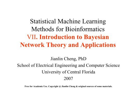
Statistical Machine Learning Methods for Bioinformatics VII ...

Statistical Machine Learning
Methods for Bioinformatics
VII. Introduction to Bayesian
Network Theory and Applications
Jianlin Cheng, PhD
School of Electrical Engineering and Computer Science
University of Central Florida
2007
Free for Academic Use. Copyright @ Jianlin Cheng & original sources of some materials.

Opening Statements
• These slides are just a quick introduction to the
Bayesian networks and their applications in
bioinformatics due to the time limit.
• For the in-depth treatment of Bayesian networks,
students are advised to read the books and papers
listed at the course web site and the Kevin
Murphy’s introduction.
• Thanks to Kevin Murphy’s excellent introduction
tutorial: http://www.cs.ubc.ca/~murphyk/Bayes/bnintro.html

Definition of Graphical Model
• Probabilistic graphical models are graphs in
which nodes represent random variables,
and the (lack of) arcs represent conditional
independence.
• It provides a compact representation of joint
probability distribution

Markov Random Fields
• Undirected graphical models (also called
Markov networks)
• Two sets of nodes A and B are
conditionally independent give a third set C
if all paths between A and B are separated
by a node C.
• Popular with the physics and vision
communities.

A
C
B
A ┴ B | C

Bayesian Networks
• Directed graphical models (also called
Belief Networks)
• Popular with AI and statistics communities.
• A model with both directed and undirected
arcs is called a chain graph

Comparison of Directed and
Undirected Graphical Models
• Independence relationship of directed graph
is more complicated.
• A -> B can encode causal relationship
• Directed models can encode deterministic
relationship, and are easier to learn (fit to
data).

Advantages of BN
• Compact & intuitive representation
• Captures causal relationships
• Efficient model learning (parameters and
structure)
• Deals with noisy data
• Integration of prior knowledge
• Effective inference algorithms
N. Friedman, 2005

Conditional Probability Distribution
• Discrete variable: CPT, conditional
probability table
C P(S=F) P(S=T)
F 0.5 0.5
T 0.9 0.1
P(C=F) P(C=T)
0.5 0.5
Cloudy
C P(R=F) P(R=T)
F 0.8 0.2
T 0.2 0.8
Sprinklet
Rain
WetGrass
S R P(W=F) P(W=T)
F F 1.0 0.0
T F 0.1 0.9
F T 0.1 0.9
T T 0.01 0.99

The Simplest Conditional
Independence in BN
• A node is independent of its ancestors given its
parents, where the ancestor / parent relationship is
with respect to some fixed topological ordering of
the nodes
• The joint probability is the product of the
conditional probability
• For previous examples: P(C, S, R, W) = P(C) *
P(S|C) * P(R|C,S) * P(W|C, S, R) = P(C) * P(S|C)
* P(R|C) * P(W|S,R).

Compact Representation of Joint
Probability
• In general, if we had n binary nodes, the full
joint would require O(2 n ) space to represent,
assuming each node has two possible
values. But the factored form would require
O(n2 k ) space to represent, where k is the
maximum fan-in of a node.
• Fewer parameters makes learning easier.

Inference
• Probabilistic inference is one of the most
common tasks we wish to solve using BN.
• Question: Suppose we observe the fact that
the grass is wet. There are two possible
causes for this: either it is raining, or the
sprinkler is on. Which is more likely?
• We can use Bayes’s rule to compute the
posterior probability of each explanation.

P(W=1) is a normalizing constant, equal to the probability (likelihood)
of the data. So we see it is more likely that the grass is wet because
it is raining.

Explaining Away
• S and R are the two causes competing to explain
the observed data.
• So if w is not observed, S and R are marginally
independent.
• If w is observed, S and R become conditionally
dependent. P(S=1|W=1, R=1) = 0.1945 <
P(S=1|W=1)
• This is called “explaining away”. In statistics, it is
known as Berkson’s paradox, or “selection bias”.

Top-Down and
Bottom-Up Reasoning
• Bottom up: In the water sprinkler example,
we had evidence of an effect (wet grass),
and inferred the most likely cause.
• Top down: We can compute the probability
that the grass will be wet given that it is
cloudy. (how causes generate effects).

Conditional Independence in BN
• Bayes Ball algorithm (due to Ross Shachter)
• Two (sets of) nodes A and B are conditionally
independent (d-separated) given a set of C if
and only if there is no way for a ball to get
from A to B in a graph, where the allowable
movements of ball are shown in the following
figures.

In the first column, when we have two arrows converging on
a node X. If X is hidden, its parents are marginally independent.
But if X is observed, the parents become dependent, and
the ball pass through. Why?

Comments
If the previous graph is
undirected, the child would
always separate the parents;
hence when converting a
directed graph to an undirected
graph, we must add links
between “unmarried” parents
who share a common child (i.e.,
“moralize” the graph) to prevent
us reading off incorrect
independence statements.
A
C
B

Example
A
B
A
B
C
C
D
Is A independent B given D?
D
Is A independent of B given C

Bayes Nets with Discrete and
Continuous Nodes
• It is possible to create Bayesian networks with
continuous valued nodes. The most common
distribution for such variable is the Gaussian.
• For discrete nodes with continuous parents, we
can use logistic / softmax distribution.
• Using multinomial, conditional Gaussians, and
softmax distribution, we can have a rich toolbox
for making complex models.
• For a good review: A Unifying Review of Linear
Gaussian Models, S. Roweis & Z. Ghahramani.
Neural Computation, 1999.

Dynamic Bayesian Networks
• DBNs are directed graphical models of
stochastic processes.
• Examples: hidden Markov models and
linear dynamical systems.

Hidden Markov Model (A New View)
q1 q2 q3 q4 …
x1 x2 x3 x4
We have “unrolled” the model for 4 “time slices” -- the structure
and parameters are assumed to repeat as the model is unrolled
further. Hence to specify a DBN, we need to define the intra-slice
topology (within a slice), the inter-slice topology (between two
slices).

Linear Dynamic Systems (LDSs)
and Kalman Filters
• A linear dynamical system (LDS) has the
same topology as an HMM, but all nodes
are assumed to have linear-Gaussian
distributions, i.e., x(t+1) = A*x(t) + w(t), w
~ N(0, Q), x(0) ~ N (init_x, init_v), y(t) =
C*x(t) + v(t), v ~ N(0, R)

The Kalman filter has been proposed as a model for how the
Brain integrates visual cues over time to infer the state of the
World, although the reality is obviously more complicated.
Kalman filter is also used in tacking of objects.

Efficient Inference Algorithms
• A simple summation of joint probability
distribution (JPD) over all variables can
answer all possible inference queries by
marginalization, but takes exponential time.
• For a Bayes net, we can sometime use the
factored representation of the JPD to do
marginalization efficiently. The key idea is to
“push sums” as far as possible when
summing out irrelevant terms.

Variable Elimination: Water Sprinkler Network

• The principle of distributing sums over
products can be generalized greatly to apply to
any commutative summing. This forms the
basis of many common algorithms, such as
Viterbi decoding and the Fast Fourier
Transform.
• The amount of work we perform when
computing a marginal is bounded by the size
of the largest term that we encounter.
Choosing a summation (elimination) ordering
to minimize this is NP-hard, although greedy
algorithms work well in practice.

Dynamic Programming and Local
Message Passing
• To compute several marginals at the same time,
we can use DP to avoid redundant computation
that would be involved if we used variable
elimination repeatedly.
• If the underlying undirected graph of the BN is
acyclic (i.e. a tree), we can use a local message
passing algorithm due to Perl. It is a generalization
of the well-known forwards-backwards algorithm
for HMMs (chains).

Local Message Passing
• If the BN has undirected cycles (as in the water sprinkler
example), local message passing algorithms run the risk of
double counting (e.g. the information from S and R
flowing into W is not independent, because it came from a
common cause, C).
• The most common approach is therefore to convert the BN
into a tree, by clustering nodes together, to form what is
called a junction tree, then running a local message
passing algorithm on the tree.
• The running time of the DP algorithm is exponential in the
size of the largest cluster (these clusters correspond to the
intermediate terms created by variable elimination). The
size is called the induced width of the graph. Minimizing
this is NP hard.

Approximation Algorithms
• Exact inference is still very slow in some
practical problems such as multivariate
time-series or image analysis due to large
induced width.
• Major approximation techniques:
Variational methods, Sampling (Monte
Carlo) methods, loopy belief propagation

Learning of BN
• The graph topology of BN
• The parameters of each CPD
• Learning structure is much harder than
learning parameters
• Learning when some of nodes are hidden
or we have missing data, is much harder
than when everything is observed.

Known Structure, Full Observability
• Maximize log-likelihood
of training data D is sum
of terms, one for each
node:
• Maximize the contribution
of the log-likelihood of
each node independently.
For discrete variables, we
just simply count the
observations.

Known Structure, Partial Observability
• When some nodes are hidden, we can use
EM algorithm to find a locally optimal
Maximum Likelihood Estimate of the
parameters
• For instance, Welch-Baum algorithm for
HMM learning. (see slides of HMM theory)

More Complicated Learning
• Unknown structure, full observability (model
selection, search the best model is NP hard. Number
of DAGs on N variables is super-exponential in N)
• Unknown structure, partial observability (Search +
EM algorithm)
• Further reading on learning:
(1) W. L. Buntine, Operations for Learning with
Graphical Models, J. AI Research, 1994
(2) D. Heckerman, A tutorial on learning with
Bayesian networks, 1996.

General Application Examples
• Microsoft Answer Wizard of Office 95, 97 and
over 30 technical support troubleshooters
• Vista system by Eric Horvitz, a decision-theoretic
system that has been used at NASA mission
control center in Houston for several years.
(provide advices on the likelihood of alternative
failures of the space shuttle’s propulsion systems)
• Quick medical reference model: model the
relationship between diseases and symptoms.

Infer the posterior probability P( disease | symptom )

Discovery of Regulatory Mechanism
/ Network of Genes
• A long term goal of Systems Biology is to
discover the causal processes among genes,
proteins, and other molecules in cells
• Can this be done (in part) by using data from high
throughput experiments, such as microarrays?
• Clustering can group genes with similar
expression patterns, but does not reveal structural
relations between genes
• Bayesian Network (BN) is a probabilistic
framework capable of learning complex relations
between genes

Learning BN from Gene Expression
Data
Measured expression level of
each gene (discretized)
Random variables
Affecting on another
Data + Prior Information
Learn parameters (conditional probabilities) from data
Learn structure (casual relation) from data
Make inference given a learned BN model
N. Friedman, 2005

Gene Bayesian Network
Gene E
Qualitative Part:
Directed acyclic Graph (DAG)
• Nodes – random variables
•Edges – direct (causal)
influence
Gene D
Gene B
Gene A
E B | P(A|E,B)
| 1 0
0 1 | 0.9 0.1
1 0 | 0.2 0.8
1 1 | 0.9 0.1
0 0 | 0.01 0.99
Gene C
Quantitative part
•Local conditional
probability

Challenges of Gene Bayesian Network
• Massive number of variables (genes)
• Small number of samples (dozens)
• Sparse networks (only a small number of
genes directly affect one another)
• Two crucial aspects: computational
complexity and statistical significance of
relations in learned models
N. Friedman, 2005

Solutions
• Sparse candidate algorithm (by Nir Friedman):
Choose a small candidate set for direct influence
for each gene. Find optimal BN constrained on
candidates. Iteratively improve candidate set.
• Bootstrap confidence estimate: use re-sampling
to generate perturbations of training data. Use the
number of times a relation (or feature) is repeated
among networks learned from these datasets to
estimate confidence of Bayesian network features.

N. Friedman, 2005
Data: 76 samples of 250 cell-cycle related genes in yeast genome
Discretized into 3 expression levels. Run 100 bootstrap using sparse learning algorithm.
Compute the confidence of features (relations). Most high confident relations make bio-senses.

Important References: BN in
Bioinformatics
•N. Friedman. Inferring cellular networks
using probabilistic graphical models,
Science, v303 p799, 6 Feb 2004.
• E. Segal et al.. Module networks: identifying
regulatory modules and their conditionspecific
regulators from gene expression
data. Nature Genetics, 2003.