

Maximally localized Wannier functions: Theory and applications
Maximally localized Wannier functions: Theory and applications
Maximally localized Wannier functions: Theory and applications

You also want an ePaper? Increase the reach of your titles
YUMPU automatically turns print PDFs into web optimized ePapers that Google loves.
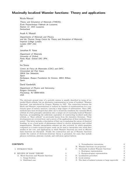
<strong>Maximally</strong> <strong>localized</strong> <strong>Wannier</strong> <strong>functions</strong>: <strong>Theory</strong> <strong>and</strong> <strong>applications</strong><br />
Nicola Marzari<br />
<strong>Theory</strong> <strong>and</strong> Simulation of Materials (THEOS),<br />
École Polytechnique Fédérale de Lausanne,<br />
Station 12, 1015 Lausanne,<br />
Switzerl<strong>and</strong><br />
Arash A. Mostofi<br />
Departments of Materials <strong>and</strong> Physics,<br />
<strong>and</strong> the Thomas Young Centre for <strong>Theory</strong> <strong>and</strong> Simulation of Materials,<br />
Imperial College London,<br />
London SW7 2AZ,<br />
UK<br />
Jonathan R. Yates<br />
Department of Materials,<br />
University of Oxford,<br />
Parks Road, Oxford OX1 3PH,<br />
UK<br />
Ivo Souza<br />
Centro de Física de Materiales (CSIC) <strong>and</strong> DIPC,<br />
Universidad del País Vasco,<br />
20018 San Sebastián,<br />
Spain<br />
Ikerbasque, Basque Foundation for Science, 48011 Bilbao,<br />
Spain<br />
David V<strong>and</strong>erbilt<br />
Department of Physics <strong>and</strong> Astronomy,<br />
Rutgers University,<br />
Piscataway, NJ 08854-8019,<br />
USA<br />
The electronic ground state of a periodic system is usually described in terms of extended<br />
Bloch orbitals, but an alternative representation in terms of <strong>localized</strong> “<strong>Wannier</strong><br />
<strong>functions</strong>” was introduced by Gregory <strong>Wannier</strong> in 1937. The connection between the<br />
Bloch <strong>and</strong> <strong>Wannier</strong> representations is realized by families of transformations in a continuous<br />
space of unitary matrices, carrying a large degree of arbitrariness. Since 1997,<br />
methods have been developed that allow one to iteratively transform the extended Bloch<br />
orbitals of a first-principles calculation into a unique set of maximally <strong>localized</strong> <strong>Wannier</strong><br />
<strong>functions</strong>, accomplishing the solid-state equivalent of constructing <strong>localized</strong> molecular<br />
orbitals, or “Boys orbitals” as previously known from the chemistry literature. These<br />
developments are reviewed here, <strong>and</strong> a survey of the <strong>applications</strong> of these methods is presented.<br />
This latter includes a description of their use in analyzing the nature of chemical<br />
bonding, or as a local probe of phenomena related to electric polarization <strong>and</strong> orbital<br />
magnetization. <strong>Wannier</strong> interpolation schemes are also reviewed, by which quantities<br />
computed on a coarse reciprocal-space mesh can be used to interpolate onto much finer<br />
meshes at low cost, <strong>and</strong> <strong>applications</strong> in which <strong>Wannier</strong> <strong>functions</strong> are used as efficient<br />
basis <strong>functions</strong> are discussed. Finally the construction <strong>and</strong> use of <strong>Wannier</strong> <strong>functions</strong><br />
outside the context of electronic-structure theory is presented, for cases that include<br />
phonon excitations, photonic crystals, <strong>and</strong> cold-atom optical lattices.<br />
CONTENTS<br />
I. INTRODUCTION 2<br />
II. REVIEW OF BASIC THEORY 3<br />
A. Bloch <strong>functions</strong> <strong>and</strong> <strong>Wannier</strong> <strong>functions</strong> 3<br />
1. Gauge freedom 4<br />
2. Multib<strong>and</strong> case 5<br />
3. Normalization conventions 6<br />
B. <strong>Wannier</strong> <strong>functions</strong> via projection 6<br />
C. <strong>Maximally</strong> <strong>localized</strong> <strong>Wannier</strong> <strong>functions</strong> 7<br />
1. Real-space representation 8<br />
2. Reciprocal-space representation 8<br />
D. Localization procedure 9<br />
E. Local minima 9<br />
F. The limit of isolated systems or large supercells 10
2<br />
1. Real-space formulation for isolated systems 10<br />
2. Γ-point formulation for large supercells 11<br />
G. Exponential localization 12<br />
H. Hybrid <strong>Wannier</strong> <strong>functions</strong> 12<br />
I. Entangled b<strong>and</strong>s 12<br />
1. Subspace selection via projection 13<br />
2. Subspace selection via optimal smoothness 14<br />
3. Iterative minimization of Ω I 16<br />
4. Localization <strong>and</strong> local minima 16<br />
J. Many-body generalizations 17<br />
III. RELATION TO OTHER LOCALIZED ORBITALS 17<br />
A. Alternative localization criteria 17<br />
B. Minimal-basis orbitals 19<br />
1. Quasiatomic orbitals 19<br />
2. NMTO <strong>and</strong> Downfolding 20<br />
C. Comparative discussion 21<br />
D. Non-orthogonal orbitals <strong>and</strong> linear scaling 21<br />
E. Other local representations 22<br />
IV. ANALYSIS OF CHEMICAL BONDING 23<br />
A. Crystalline solids 24<br />
B. Complex <strong>and</strong> amorphous phases 25<br />
C. Defects 26<br />
D. Chemical interpretation 27<br />
E. MLWFs in first-principles molecular dynamics 27<br />
V. ELECTRIC POLARIZATION AND ORBITAL<br />
MAGNETIZATION 28<br />
A. <strong>Wannier</strong> <strong>functions</strong>, electric polarization, <strong>and</strong><br />
localization 29<br />
1. Relation to Berry-phase theory of polarization 29<br />
2. Insulators in finite electric field 30<br />
3. <strong>Wannier</strong> spread <strong>and</strong> localization in insulators 30<br />
4. Many-body generalizations 30<br />
B. Local polar properties <strong>and</strong> dielectric response 31<br />
1. Polar properties <strong>and</strong> dynamical charges of<br />
crystals 31<br />
2. Local dielectric response in layered systems 32<br />
3. Condensed molecular phases <strong>and</strong> solvation 33<br />
C. Magnetism <strong>and</strong> orbital currents 34<br />
1. Magnetic insulators 34<br />
2. Orbital magnetization <strong>and</strong> NMR 34<br />
3. Berry connection <strong>and</strong> curvature 35<br />
4. Topological insulators <strong>and</strong> orbital magnetoelectric<br />
response 35<br />
VI. WANNIER INTERPOLATION 36<br />
A. B<strong>and</strong>-structure interpolation 36<br />
1. Spin-orbit-coupled b<strong>and</strong>s of bcc Fe 37<br />
2. B<strong>and</strong> structure of a metallic carbon nanotube 38<br />
3. GW quasiparticle b<strong>and</strong>s 39<br />
4. Surface b<strong>and</strong>s of topological insulators 39<br />
B. B<strong>and</strong> derivatives 41<br />
1. Application to transport coefficients 41<br />
C. Berry curvature <strong>and</strong> anomalous Hall conductivity 42<br />
D. Electron-phonon coupling 44<br />
VII. WANNIER FUNCTIONS AS BASIS FUNCTIONS 45<br />
A. WFs as a basis for large-scale calculations 45<br />
1. MLWFs as electronic-structure building blocks 46<br />
2. Quantum transport 46<br />
3. Semi-empirical potentials 48<br />
4. Improving system-size scaling 48<br />
B. WFs as a basis for strongly-correlated systems 49<br />
1. First-principles model Hamiltonians 50<br />
2. Self-interaction <strong>and</strong> DFT + Hubbard U 51<br />
VIII. WANNIER FUNCTIONS IN OTHER CONTEXTS 51<br />
A. Phonons 51<br />
B. Photonic crystals 53<br />
C. Cold atoms in optical lattices 54<br />
IX. SUMMARY AND PROSPECTS 56<br />
References 56<br />
I. INTRODUCTION<br />
In the independent-particle approximation, the electronic<br />
ground state of a system is determined by specifying<br />
a set of one-particle orbitals <strong>and</strong> their occupations.<br />
For the case of periodic system, these one-particle<br />
orbitals are normally taken to be the Bloch <strong>functions</strong><br />
ψ nk (r) that are labeled, according to Bloch’s theorem, by<br />
a crystal momentum k lying inside the Brillouin zone <strong>and</strong><br />
a b<strong>and</strong> index n. Although this choice is by far the most<br />
widely used in electronic-structure calculations, alternative<br />
representations are possible. In particular, to arrive<br />
at the <strong>Wannier</strong> representation (des Cloizeaux, 1963;<br />
Kohn, 1959; <strong>Wannier</strong>, 1937), one carries out a unitary<br />
transformation from the Bloch <strong>functions</strong> to a set of <strong>localized</strong><br />
“<strong>Wannier</strong> <strong>functions</strong>” (WFs) labeled by a cell index<br />
R <strong>and</strong> a b<strong>and</strong>-like index n, such that in a crystal the<br />
WFs at different R are translational images of one another.<br />
Unlike Bloch <strong>functions</strong>, WFs are not eigenstates<br />
of the Hamiltonian; in selecting them, one trades off localization<br />
in energy for localization in space.<br />
In the earlier solid-state theory literature, WFs were<br />
typically introduced in order to carry out some formal<br />
derivation – for example, of the effective-mass treatment<br />
of electron dynamics, or of an effective spin Hamiltonian<br />
– but actual calculations of the WFs were rarely performed.<br />
The history is rather different in the chemistry<br />
literature, where “<strong>localized</strong> molecular orbitals” (LMO’s)<br />
(Boys, 1960, 1966; Edmiston <strong>and</strong> Ruedenberg, 1963; Foster<br />
<strong>and</strong> Boys, 1960a,b) have played a significant role in<br />
computational chemistry since its early days. Chemists<br />
have emphasized that such a representation can provide<br />
an insightful picture of the nature of the chemical bond<br />
in a material — otherwise missing from the picture of<br />
extended eigenstates — or can serve as a compact basis<br />
set for high-accuracy calculations.<br />
The actual implementation of <strong>Wannier</strong>’s vision in<br />
the context of first-principles electronic-structure calculations,<br />
such as those carried out in the Kohn-Sham<br />
framework of density-functional theory (Kohn <strong>and</strong> Sham,<br />
1965), has instead been slower to unfold. A major reason<br />
for this is that WFs are strongly non-unique. This<br />
is a consequence of the phase indeterminacy that Bloch<br />
orbitals ψ nk have at every wavevector k – or, more generally,<br />
the “gauge” indeterminacy associated with the freedom<br />
to apply any arbitrary unitary transformation to the<br />
occupied Bloch states at each k. This second indeterminacy<br />
is all the more troublesome in the common case<br />
of degeneracy for the occupied b<strong>and</strong>s at certain highsymmetry<br />
points in the Brillouin zone, making a par-
3<br />
tition into separate “b<strong>and</strong>s”, that could separately be<br />
transformed in <strong>Wannier</strong> <strong>functions</strong>, problematic. Therefore,<br />
even before one could attempt to compute the WFs<br />
for a given material, one had first to resolve the question<br />
of which states to use to compute WFs.<br />
An important development in this regard was the introduction<br />
by Marzari <strong>and</strong> V<strong>and</strong>erbilt (1997) of a “maximal<br />
localization” criterion for identifying a unique set of WFs<br />
for a given crystalline insulator. The approach is similar<br />
in spirit to the construction of LMO’s in chemistry,<br />
but its implementation in the solid-state context required<br />
significant developments, due to the ill-conditioned nature<br />
of the position operator in periodic systems (Nenciu,<br />
1991), that was clarified in the context of the “modern<br />
theory” of polarization (King-Smith <strong>and</strong> V<strong>and</strong>erbilt,<br />
1993; Resta, 1994). Marzari <strong>and</strong> V<strong>and</strong>erbilt showed that<br />
the minimization of a localization functional corresponding<br />
to the sum of the second-moment spread of each <strong>Wannier</strong><br />
charge density about its own center of charge was<br />
both formally attractive <strong>and</strong> computationally tractable.<br />
In a related development, Souza et al. (2001) generalized<br />
the method to h<strong>and</strong>le the case in which one wants to<br />
construct a set of WFs that spans a subspace containing,<br />
e.g., the partially occupied b<strong>and</strong>s of a metal.<br />
These developments touched off a transformational<br />
shift in which the computational electronic-structure<br />
community started constructing maximally-<strong>localized</strong><br />
WFs (MLWFs) explicitly <strong>and</strong> using these for different<br />
purposes. The reasons are manifold: First, WFs, akin<br />
to LMO’s in molecules, provide an insightful chemical<br />
analysis of the nature of bonding, <strong>and</strong> its evolution during,<br />
say, a chemical reaction. As such, they have become<br />
an established tool in the post-processing of electronicstructure<br />
calculations. More interestingly, there are formal<br />
connections between the centers of charge of the<br />
WFs <strong>and</strong> the Berry phases of the Bloch <strong>functions</strong> as<br />
they are carried around the Brillouin zone. This connection<br />
is embodied in the microscopic modern theory<br />
of polarization, alluded to above, <strong>and</strong> has led to important<br />
advances in the characterization <strong>and</strong> underst<strong>and</strong>ing<br />
of dielectric response <strong>and</strong> polarization in materials.<br />
Of broader interest to the entire condensed matter community<br />
is the use of WFs in the construction of model<br />
Hamiltonians for, e.g., correlated-electron <strong>and</strong> magnetic<br />
systems. An alternative use of WFs as <strong>localized</strong>, transferable<br />
building blocks has taken place in the theory of ballistic<br />
(L<strong>and</strong>auer) transport, where Green’s <strong>functions</strong> <strong>and</strong><br />
self-energies can be constructed effectively in a <strong>Wannier</strong><br />
basis, or that of first-principles tight-binding Hamiltonians,<br />
where chemically-accurate Hamiltonians are constructed<br />
directly on the <strong>Wannier</strong> basis, rather than fitted<br />
or inferred from macroscopic considerations. Finally, the<br />
ideas that were developed for electronic WFs have also<br />
seen application in very different contexts. For example,<br />
MLWF’s have been used in the theoretical analysis of<br />
phonons, photonic crystals, cold atom lattices, <strong>and</strong> the<br />
local dielectric responses of insulators.<br />
Here we review these developments. We first introduce<br />
the transformation from Bloch <strong>functions</strong> to WFs in<br />
Sec. II, discussing their gauge freedom <strong>and</strong> the methods<br />
developed for constructing WFs through projection or<br />
maximal localization. A “disentangling procedure” for<br />
constructing WFs for a non-isolated set of b<strong>and</strong>s (e.g.,<br />
in metals) is also described. In Sec. III we discuss variants<br />
of these procedures in which different localization<br />
criteria or different algorithms are used, <strong>and</strong> discuss the<br />
relationship to “downfolding” <strong>and</strong> linear-scaling methods.<br />
Sec. IV describes how the calculation of WFs has<br />
proved to be a useful tool for analyzing the nature of the<br />
chemical bonding in crystalline, amorphous, <strong>and</strong> defective<br />
systems. Of particular importance is the ability to<br />
use WFs as a local probe of electric polarization, as described<br />
in Sec. V. There we also discuss how the <strong>Wannier</strong><br />
representation has been useful in describing orbital magnetization,<br />
NMR chemical shifts, orbital magnetoelectric<br />
responses, <strong>and</strong> topological insulators. Sec. VI describes<br />
<strong>Wannier</strong> interpolation schemes, by which quantities computed<br />
on a relatively coarse k-space mesh can be used<br />
to interpolate faithfully onto an arbitrarily fine k-space<br />
mesh at relatively low cost. In Sec. VII we discuss <strong>applications</strong><br />
in which the WFs are used as an efficient basis<br />
for the calculations of quantum transport properties, the<br />
derivation of semiempirical potentials, <strong>and</strong> for describing<br />
strongly-correlated systems. Sec. VIII contains a brief<br />
discussion of the construction <strong>and</strong> use of WFs in contexts<br />
other than electronic-structure theory, including for<br />
phonons in ordinary crystals, photonic crystals, <strong>and</strong> cold<br />
atoms in optical lattices. Finally, Sec. IX provides a short<br />
summary <strong>and</strong> conclusions.<br />
II. REVIEW OF BASIC THEORY<br />
A. Bloch <strong>functions</strong> <strong>and</strong> <strong>Wannier</strong> <strong>functions</strong><br />
Electronic structure calculations are often carried out<br />
using periodic boundary conditions. This is the most<br />
natural choice for the study of perfect crystals, <strong>and</strong> also<br />
applies to the common use of periodic supercells for the<br />
study of non-periodic systems such as liquids, interfaces,<br />
<strong>and</strong> defects. The one-particle effective Hamiltonian H<br />
then commutes with the lattice-translation operator T R ,<br />
allowing one to choose as common eigenstates the Bloch<br />
orbitals | ψ nk ⟩:<br />
[ H, T R ] = 0 ⇒ ψ nk (r) = u nk (r) e ik·r , (1)<br />
where u nk (r) has the periodicity of the Hamiltonian.<br />
Several Bloch <strong>functions</strong> are sketched on the left-h<strong>and</strong><br />
side of Fig. 1 for a toy model in which the b<strong>and</strong> of interest<br />
is composed of p-like orbitals centered on each atom.<br />
For the moment, we suppose that this b<strong>and</strong> is an isolated<br />
b<strong>and</strong>, i.e., it remains separated by a gap from the
4<br />
Bloch <strong>functions</strong><br />
ψ k0<br />
(x)<br />
<strong>Wannier</strong> <strong>functions</strong><br />
w 0<br />
(x)<br />
It is easily shown that the | Rn ⟩ form an orthonormal<br />
set (see Sec. II.A.3) <strong>and</strong> that two WFs | Rn ⟩ <strong>and</strong> | R ′ n ⟩<br />
transform into each other under translation by the lattice<br />
vector R − R ′ (Blount, 1962). Eq. (3) takes the form of<br />
a Fourier transform, <strong>and</strong> its inverse transform is<br />
ψ k1<br />
(x)<br />
w 1<br />
(x)<br />
| ψ nk ⟩ = ∑ R<br />
e ik·R |Rn⟩ (4)<br />
ψ k2<br />
(x)<br />
w 2<br />
(x)<br />
FIG. 1 (Color online) Transformation from Bloch <strong>functions</strong> to<br />
<strong>Wannier</strong> <strong>functions</strong> (WFs). Left: Real-space representation of<br />
three of the Bloch <strong>functions</strong> e ikx u k (x) associated with a single<br />
b<strong>and</strong> in 1D, for three different values of the wavevector k.<br />
Filled circles indicate lattice vectors, <strong>and</strong> thin (green) lines the<br />
e ikx envelopes of each Bloch function. Right: WFs associated<br />
with the same b<strong>and</strong>, forming periodic images of one another.<br />
The two sets of Bloch <strong>functions</strong> at every k in the Brillouin<br />
zone <strong>and</strong> WFs at every lattice vector span the same Hilbert<br />
space.<br />
b<strong>and</strong>s below <strong>and</strong> above at all k. Since Bloch <strong>functions</strong><br />
at different k have different envelope <strong>functions</strong> e ik·r , one<br />
can expect to be able to build a <strong>localized</strong> “wave packet”<br />
by superposing Bloch <strong>functions</strong> of different k. To get a<br />
very <strong>localized</strong> wave packet in real space, we need to use<br />
a very broad superposition in k space. But k lives in the<br />
periodic Brillouin zone, so the best we can do is to choose<br />
equal amplitudes all across the Brillouin zone. Thus, we<br />
can construct<br />
w 0 (r) =<br />
V<br />
(2π) 3 ∫BZ<br />
dk ψ nk (r) , (2)<br />
where V is the real-space primitive cell volume <strong>and</strong> the<br />
integral is carried over the Brillouin zone (BZ). (See<br />
Sec. II.A.3 for normalization conventions.) Equation (2)<br />
can be interpreted as the WF located in the home unit<br />
cell, as sketched in the top-right panel of Fig. 1.<br />
More generally, we can insert a phase factor e −ik·R into<br />
the integr<strong>and</strong> of Eq. (2), where R is a real-space lattice<br />
vector; this has the effect of translating the real-space<br />
WF by R, generating additional WFs such as w 1 <strong>and</strong><br />
w 2 sketched in Fig. 1. Switching to the Dirac bra-ket<br />
notation <strong>and</strong> introducing the notation that Rn refers to<br />
the WF w nR in cell R associated with b<strong>and</strong> n, WFs can<br />
be constructed according to (<strong>Wannier</strong>, 1937)<br />
|Rn⟩ =<br />
V<br />
(2π) 3 ∫BZ<br />
dk e −ik·R | ψ nk ⟩ . (3)<br />
(see Sec. II.A.3). Any of the Bloch <strong>functions</strong> on the left<br />
side of Fig. 1 can thus be built up by linearly superposing<br />
the WFs shown on the right side, when the appropriate<br />
phases e ik·R are used.<br />
The transformations of Eqs. (3) <strong>and</strong> (4) constitute<br />
a unitary transformation between Bloch <strong>and</strong> <strong>Wannier</strong><br />
states. Thus, both sets of states provide an equally valid<br />
description of the b<strong>and</strong> subspace, even if the WFs are<br />
not Hamiltonian eigenstates. For example, the charge<br />
density obtained by summing the squares of the Bloch<br />
<strong>functions</strong> |ψ nk ⟩ or the WFs |Rn⟩ is identical; a similar<br />
reasoning applies to the trace of any one-particle operator.<br />
The equivalence between the Bloch <strong>and</strong> the <strong>Wannier</strong><br />
representations can also be made manifest by expressing<br />
the b<strong>and</strong> projection operator P in both representations,<br />
i.e., as<br />
P =<br />
V<br />
(2π) 3 ∫BZ<br />
dk |ψ nk ⟩⟨ψ nk | = ∑ R<br />
|Rn⟩⟨Rn| . (5)<br />
WFs thus provide an attractive option for representing<br />
the space spanned by a Bloch b<strong>and</strong> in a crystal, being<br />
<strong>localized</strong> while still carrying the same information contained<br />
in the Bloch <strong>functions</strong>.<br />
1. Gauge freedom<br />
However, the theory of WFs is made more complex<br />
by the presence of a “gauge freedom” that exists in the<br />
definition of the ψ nk . In fact, we can replace<br />
or equivalently,<br />
| ˜ψ nk ⟩ = e iφn(k) | ψ nk ⟩ , (6)<br />
| ũ nk ⟩ = e iφ n(k) | u nk ⟩ , (7)<br />
without changing the physical description of the system,<br />
with φ n (k) being any real function that is periodic in<br />
reciprocal space. 1 A smooth gauge could, e.g., be defined<br />
1 More precisely, the condition is that φ n (k+G) = φ n (k)+G·∆R<br />
for any reciprocal-lattice translation G, where ∆R is a real-space<br />
lattice vector. This allows for the possibility that φ n may shift<br />
by 2π times an integer upon translation by G; the vector ∆R<br />
expresses the corresponding shift in the position of the resulting<br />
WF.
5<br />
such that ∇ k |u nk ⟩ is well defined at all k. Henceforth<br />
we shall assume that the Bloch <strong>functions</strong> on the righth<strong>and</strong><br />
side of Eq. (3) belong to a smooth gauge, since<br />
we would not get well-<strong>localized</strong> WFs on the left-h<strong>and</strong><br />
side otherwise. This is typical of Fourier transforms: the<br />
smoother the reciprocal-space object, the more <strong>localized</strong><br />
the resulting real-space object, <strong>and</strong> vice versa.<br />
One way to see this explicitly is to consider the R = 0<br />
home-cell w n0 (r) evaluated at a distant point r; using<br />
Eq. (1) in Eq. (3), this is given by ∫ BZ<br />
u nk(r)e ik·r dk,<br />
which will be small due to cancellations arising from the<br />
rapid variation of the exponential factor, provided that<br />
u nk is a smooth function of k (Blount, 1962).<br />
It is important to realize that the gauge freedom of<br />
Eqs. (6) <strong>and</strong> (7) propagates into the WFs. That is,<br />
different choices of smooth gauge correspond to different<br />
sets of WFs having in general different shapes <strong>and</strong><br />
spreads. In this sense, the WFs are “more non-unique”<br />
than the Bloch <strong>functions</strong>, which only acquire a phase<br />
change. We also emphasize that there is no “preferred<br />
gauge” assigned by the Schrödinger equation to the Bloch<br />
orbitals. Thus, the non-uniqueness of the WFs resulting<br />
from Eq. (3) is unavoidable.<br />
2. Multib<strong>and</strong> case<br />
Before discussing how this non-uniqueness might be<br />
resolved, we first relax the condition that b<strong>and</strong> n be a<br />
single isolated b<strong>and</strong>, <strong>and</strong> consider instead a manifold of<br />
J b<strong>and</strong>s that remain separated with respect to any lower<br />
or higher b<strong>and</strong>s outside the manifold. Internal degeneracies<br />
<strong>and</strong> crossings among the J b<strong>and</strong>s may occur in<br />
general. In the simplest case this manifold corresponds<br />
to the occupied b<strong>and</strong>s of an insulator, but more generally<br />
it consists of any set of b<strong>and</strong>s that is separated by a gap<br />
from both lower <strong>and</strong> higher b<strong>and</strong>s everywhere in the Brillouin<br />
zone. Traces over this b<strong>and</strong> manifold are invariant<br />
with respect to any unitary transformation among the J<br />
occupied Bloch orbitals at a given wavevector, so it is<br />
natural to generalize the notion of a “gauge transformation”<br />
to<br />
| ˜ψ nk ⟩ =<br />
J∑<br />
m=1<br />
U (k)<br />
mn | ψ mk ⟩ . (8)<br />
Here U mn<br />
(k) is a unitary matrix of dimension J that is<br />
periodic in k, with Eq. (6) corresponding to the special<br />
case of a diagonal U matrix. It follows that the projection<br />
operator onto this b<strong>and</strong> manifold at wavevector k,<br />
P k =<br />
J∑<br />
|ψ nk ⟩⟨ψ nk | =<br />
n=1<br />
J∑<br />
| ˜ψ nk ⟩⟨ ˜ψ nk | (9)<br />
n=1<br />
is invariant, even though the | ˜ψ nk ⟩ resulting from Eq. (8)<br />
are no longer generally eigenstates of H, <strong>and</strong> n is no<br />
longer a b<strong>and</strong> index in the usual sense.<br />
FIG. 2 (Color online) <strong>Maximally</strong>-<strong>localized</strong> <strong>Wannier</strong> <strong>functions</strong><br />
(MLWFs) constructed from the four valence b<strong>and</strong>s of Si (left)<br />
<strong>and</strong> GaAs (right; Ga at upper right, As at lower left), displaying<br />
the character of σ-bonded combinations of sp 3 hybrids.<br />
Isosurfaces of different shades of gray (red, blue) correspond<br />
to two opposite values for the amplitudes of the real-valued<br />
MLWFs.<br />
Our goal is again to construct WFs out of these transformed<br />
Bloch <strong>functions</strong> using Eq. (3). Figs. 2(a) <strong>and</strong> (b)<br />
show, for example, what the result might eventually look<br />
like for the case of the four occupied valence b<strong>and</strong>s of Si<br />
or GaAs, respectively. From these four b<strong>and</strong>s, one obtains<br />
four equivalent WFs per unit cell, each <strong>localized</strong> on<br />
one of the four nearest-neighbor Si-Si or Ga-As bonds.<br />
The presence of a bond-centered inversion symmetry for<br />
Si, but not GaAs, is clearly reflected in the shapes of the<br />
WFs.<br />
Once again, we emphasize that the gauge freedom expressed<br />
in Eq. (8) implies that the WFs are strongly nonunique.<br />
This is illustrated in Fig. 3, which shows an alternative<br />
construction of WFs for GaAs. The WF on the<br />
left was constructed from the lowest valence b<strong>and</strong> n=1,<br />
while the one on the right is one of three constructed from<br />
b<strong>and</strong>s n=2-4. The former has primarily As s character<br />
<strong>and</strong> the latter has primarily As p character, although<br />
both (<strong>and</strong> especially the latter) contain some Ga s <strong>and</strong><br />
p character as well. The WFs of Figs. 2(b) <strong>and</strong> Fig. 3<br />
are related to each other by a certain manifold of 4×4<br />
unitary matrices U nm (k) relating their Bloch transforms in<br />
the manner of Eq. (8).<br />
However, before we can arrive at well-<strong>localized</strong> WFs<br />
like those shown in Figs. 2 <strong>and</strong> 3, we again have to address<br />
questions of smoothness of the gauge choice expressed in<br />
Eq. (8). This issue is even more profound in the present<br />
multib<strong>and</strong> case, since this smoothness criterion is generally<br />
incompatible with the usual construction of Bloch<br />
<strong>functions</strong>. That is, if we simply insert the usual Bloch<br />
{<br />
L Γ X K Γ<br />
}<br />
FIG. 3 (Color online) MLWFs constructed from the s b<strong>and</strong><br />
(left) or from the three p b<strong>and</strong>s (right) of GaAs.
6<br />
<strong>functions</strong> |ψ nk ⟩, defined to be eigenstates of H, into the<br />
right-h<strong>and</strong> side of Eq. (3), it is generally not possible to<br />
produce well-<strong>localized</strong> WFs. The problem arises when<br />
there are degeneracies among the b<strong>and</strong>s in question at<br />
certain locations in the Brillouin zone. Consider, for example,<br />
what happens if we try to construct a single WF<br />
from the highest occupied b<strong>and</strong> n = 4 in GaAs. This<br />
would be doomed to failure, since this b<strong>and</strong> becomes degenerate<br />
with b<strong>and</strong>s two <strong>and</strong> three at the zone center,<br />
Γ, as shown in Fig. 3. As a result, b<strong>and</strong> four is nonanalytic<br />
in k in the vicinity of Γ. The Fourier transform<br />
of Eq. (3) would then result in a poorly <strong>localized</strong> object<br />
having power-law tails in real space.<br />
In such cases, therefore, the extra unitary mixing expressed<br />
in Eq. (8) is m<strong>and</strong>atory, even if it may be optional<br />
in the case of a set of discrete b<strong>and</strong>s that do not<br />
touch anywhere in the BZ. So, generally speaking, our<br />
procedure must be that we start from a set of Hamiltonian<br />
eigenstates |ψ nk ⟩ that are not per se smooth in k,<br />
<strong>and</strong> introduce unitary rotations U mn (k) that “cancel out”<br />
the discontinuities in such a way that smoothness is restored,<br />
i.e., that the resulting | ˜ψ nk ⟩ of Eq. (8) obey the<br />
smoothness condition that ∇ k | ˜ψ nk ⟩ remains regular at<br />
all k. Then, when these | ˜ψ nk ⟩ are inserted into Eq. (3)<br />
in place of the |ψ nk ⟩, well-<strong>localized</strong> WFs should result.<br />
Explicitly, this results in WFs constructed according to<br />
| Rn ⟩ = V<br />
(2π)<br />
∫BZ<br />
3 dk e −ik·R<br />
J∑<br />
m=1<br />
U (k)<br />
mn | ψ mk ⟩ . (10)<br />
The question remains how to choose the unitary rotations<br />
U mn (k) so as to accomplish this task. We will see that<br />
one way to do this is to use a projection technique, as<br />
outlined in the next section. Ideally, however, we would<br />
like the construction to result in WFs that are “maximally<br />
<strong>localized</strong>” according to some criterion. Methods<br />
for accomplishing this are discussed in Sec. II.C<br />
3. Normalization conventions<br />
In the above equations, formulated for continuous k,<br />
we have adopted the convention that Bloch <strong>functions</strong> are<br />
normalized to one unit cell, ∫ V dr |ψ nk(r)| 2 = 1, even<br />
though they extend over the entire crystal. We also define<br />
⟨f|g⟩ as the integral of f ∗ g over all space. With<br />
this notation, ⟨ψ nk |ψ nk ⟩ is not unity; instead, it diverges<br />
according to the rule<br />
⟨ψ nk |ψ mk ′⟩ = (2π)3<br />
V<br />
δ nm δ 3 (k − k ′ ) . (11)<br />
With these conventions it is easy to check that the WFs<br />
in Eqs. (3-4) are properly normalized, i.e., ⟨Rn|R ′ m⟩ =<br />
δ RR ′ δ nm .<br />
It is often more convenient to work on a discrete uniform<br />
k mesh instead of continuous k space. 2 Letting N<br />
be the number of unit cells in the periodic supercell, or<br />
equivalently, the number of mesh points in the BZ, it is<br />
possible to keep the conventions close to the continuous<br />
case by defining the Fourier transform pair as<br />
|ψ nk ⟩ = ∑ e ik·R |Rn⟩<br />
R<br />
⇕ (12)<br />
|Rn⟩ = 1 ∑<br />
e −ik·R |ψ nk ⟩<br />
N<br />
k<br />
with ⟨ψ nk |ψ mk ′⟩ = Nδ nm δ kk ′, so that Eq. (5) becomes,<br />
after generalizing to the multib<strong>and</strong> case,<br />
P = 1 ∑<br />
|ψ nk ⟩⟨ψ nk | = ∑ |Rn⟩⟨Rn| . (13)<br />
N<br />
nR<br />
nk<br />
Another commonly used convention is to write<br />
|ψ nk ⟩ = √ 1 ∑<br />
e ik·R |Rn⟩<br />
N<br />
R<br />
⇕ (14)<br />
|Rn⟩ = √ 1 ∑<br />
e −ik·R |ψ nk ⟩<br />
N<br />
with ⟨ψ nk |ψ mk ′⟩ = δ nm δ kk ′ <strong>and</strong> Eq. (13) replaced by<br />
P = ∑ nk<br />
k<br />
|ψ nk ⟩⟨ψ nk | = ∑ nR<br />
|Rn⟩⟨Rn| . (15)<br />
In either case, it is convenient to keep the |u nk ⟩ <strong>functions</strong><br />
normalized to the unit cell, with inner products involving<br />
them, such as ⟨u mk |u nk ⟩, understood as integrals over<br />
one unit cell. In the case of Eq. (14), this means that<br />
u nk (r) = √ Ne −ik·r ψ nk (r).<br />
B. <strong>Wannier</strong> <strong>functions</strong> via projection<br />
A simple yet often effective approach for constructing<br />
a smooth gauge in k, <strong>and</strong> a corresponding set of well<strong>localized</strong><br />
WFs, is by projection - an approach that finds<br />
its roots in the analysis of des Cloizeaux (1964a). Here,<br />
as discussed, e.g., in Sec. IV.G.1 of Marzari <strong>and</strong> V<strong>and</strong>erbilt<br />
(1997), one starts from a set of J <strong>localized</strong> trial<br />
2 The discretization of k-space amounts to imposing periodic<br />
boundary conditions on the Bloch wave<strong>functions</strong> over a supercell<br />
in real space. Thus, it should be kept in mind that the WFs<br />
given by Eqs. (12) <strong>and</strong> (14) are not truly <strong>localized</strong>, as they also<br />
display the supercell periodicity (<strong>and</strong> are normalized to a supercell<br />
volume). Under these circumstances the notion of “<strong>Wannier</strong><br />
localization” refers to localization within one supercell, which is<br />
meaningful for supercells chosen large enough to ensure negligible<br />
overlap between a WF <strong>and</strong> its periodic images.
7<br />
orbitals g n (r) corresponding to some rough guess for the<br />
WFs in the home unit cell. Returning to the continuousk<br />
formulation, these g n (r) are projected onto the Bloch<br />
manifold at wavevector k to obtain<br />
J∑<br />
|ϕ nk ⟩ = |ψ mk ⟩⟨ψ mk |g n ⟩ , (16)<br />
m=1<br />
which are typically smooth in k-space, albeit not orthonormal.<br />
(The integral in ⟨ψ mk |g n ⟩ is over all space as<br />
usual.) We note that in actual practice such projection<br />
is achieved by first computing a matrix of inner products<br />
(A k ) mn = ⟨ψ mk |g n ⟩ <strong>and</strong> then using these in Eq. (16).<br />
The overlap matrix (S k ) mn = ⟨ϕ mk |ϕ nk ⟩ V = (A † k A k ) mn<br />
(where subscript V denotes an integral over one cell)<br />
is then computed <strong>and</strong> used to construct the Löwdinorthonormalized<br />
Bloch-like states<br />
| ˜ψ<br />
J∑<br />
nk ⟩ = |ϕ mk ⟩(S −1/2<br />
k<br />
) mn . (17)<br />
m=1<br />
These | ˜ψ nk ⟩ have now a smooth gauge in k, are related<br />
to the original |ψ nk ⟩ by a unitary transformation, 3 <strong>and</strong><br />
when substituted into Eq. (3) in place of the |ψ nk ⟩ result<br />
in a set of well-<strong>localized</strong> WFs. We note in passing<br />
that the | ˜ψ nk ⟩ are uniquely defined by the trial orbitals<br />
g n (r) <strong>and</strong> the chosen (isolated) manifold, since any arbitrary<br />
unitary rotation among the |ψ nk ⟩ orbitals cancels<br />
out exactly <strong>and</strong> does not affect the outcome of Eq. 16,<br />
eliminating thus any gauge freedom.<br />
We emphasize that the trial <strong>functions</strong> do not need to<br />
resemble the target WFs closely; it is often sufficient to<br />
choose simple analytic <strong>functions</strong> (e.g., spherical harmonics<br />
times Gaussians) provided they are roughly located<br />
on sites where WFs are expected to be centered <strong>and</strong> have<br />
appropriate angular character. The method is successful<br />
as long as the inner-product matrix A k does not become<br />
singular (or nearly so) for any k, which can be ensured by<br />
checking that the ratio of maximum <strong>and</strong> minimum values<br />
of det S k in the Brillouin zone does not become too<br />
large. For example, spherical (s-like) Gaussians located<br />
at the bond centers will suffice for the construction of<br />
well-<strong>localized</strong> WFs, akin to those shown in Fig. 2, spanning<br />
the four occupied valence b<strong>and</strong>s of semiconductors<br />
such as Si <strong>and</strong> GaAs.<br />
C. <strong>Maximally</strong> <strong>localized</strong> <strong>Wannier</strong> <strong>functions</strong><br />
The projection method described in the previous subsection<br />
has been used by many authors (Ku et al., 2002;<br />
3 One can prove that this transformation is unitary by performing<br />
the singular value decomposition A = ZDW † , with Z <strong>and</strong> W<br />
unitary <strong>and</strong> D real <strong>and</strong> diagonal. It follows that A(A † A) −1/2 is<br />
equal to ZW † , <strong>and</strong> thus unitary.<br />
Lu et al., 2004; Qian et al., 2008; Stephan et al., 2000),<br />
as has a related method involving downfolding of the<br />
b<strong>and</strong> structure onto a minimal basis (Andersen <strong>and</strong> Saha-<br />
Dasgupta, 2000; Zurek et al., 2005); some of these approaches<br />
will also be discussed in Sec. III.B. Other authors<br />
have made use of symmetry considerations, analyticity<br />
requirements, <strong>and</strong> variational procedures (Smirnov<br />
<strong>and</strong> Usvyat, 2001; Sporkmann <strong>and</strong> Bross, 1994, 1997).<br />
A very general <strong>and</strong> now widely used approach, however,<br />
has been that developed by Marzari <strong>and</strong> V<strong>and</strong>erbilt<br />
(1997) in which localization is enforced by introducing a<br />
well-defined localization criterion, <strong>and</strong> then refining the<br />
U mn (k) in order to satisfy that criterion. We first give an<br />
overview of this approach, <strong>and</strong> then provide details in the<br />
following subsections.<br />
First, the localization functional<br />
Ω = ∑ n<br />
= ∑ n<br />
[<br />
⟨ 0n | r 2 | 0n ⟩ − ⟨ 0n | r | 0n ⟩ 2 ]<br />
[<br />
⟨r 2 ⟩ n − ¯r 2 n]<br />
(18)<br />
is defined, measuring of the sum of the quadratic spreads<br />
of the J WFs in the home unit cell around their centers.<br />
This turns out to be the solid-state equivalent of the<br />
Foster-Boys criterion of quantum chemistry (Boys, 1960,<br />
1966; Foster <strong>and</strong> Boys, 1960a,b). The next step is to<br />
express Ω in terms of the Bloch <strong>functions</strong>. This requires<br />
some care, since expectation values of the position operator<br />
are not well defined in the Bloch representation. The<br />
needed formalism will be discussed briefly in Sec. II.C.1<br />
<strong>and</strong> more extensively in Sec. V.A.1, with much of the conceptual<br />
work stemming from the earlier development the<br />
modern theory of polarization (Blount, 1962; King-Smith<br />
<strong>and</strong> V<strong>and</strong>erbilt, 1993; Resta, 1992, 1994; V<strong>and</strong>erbilt <strong>and</strong><br />
King-Smith, 1993).<br />
Once a k-space expression for Ω has been derived, maximally<br />
<strong>localized</strong> WFs are obtained by minimizing it with<br />
respect to the U mn (k) appearing in Eq. (10). This is done<br />
as a post-processing step after a conventional electronicstructure<br />
calculation has been self-consistently converged<br />
<strong>and</strong> a set of ground-state Bloch orbitals | ψ mk ⟩ has been<br />
chosen once <strong>and</strong> for all. The U mn (k) are then iteratively refined<br />
in a direct minimization procedure of the localization<br />
functional that is outlined in Sec. II.D below. This<br />
procedure also provides the expectation values ⟨r 2 ⟩ n <strong>and</strong><br />
¯r n ; the latter, in particular, are the primary quantities<br />
needed to compute many of the properties, such as the<br />
electronic polarization, discussed in Sec. V. If desired,<br />
the resulting U mn (k) can also be used to construct explicitly<br />
the maximally <strong>localized</strong> WFs via Eq. (10). This step<br />
is typically only necessary, however, if one wants to visualize<br />
the resulting WFs or to use them as basis <strong>functions</strong><br />
for some subsequent analysis.
8<br />
1. Real-space representation<br />
An interesting consequence stemming from the choice<br />
of (18) as the localization functional is that it allows<br />
a natural decomposition of the functional into gaugeinvariant<br />
<strong>and</strong> gauge-dependent parts. That is, we can<br />
write<br />
where<br />
<strong>and</strong><br />
Ω I = ∑ n<br />
[<br />
Ω = Ω I + ˜Ω (19)<br />
⟨ 0n | r 2 | 0n ⟩ − ∑ Rm<br />
˜Ω = ∑ n<br />
∑<br />
Rm≠0n<br />
∣<br />
∣⟨Rm|r|0n⟩ ∣ ]<br />
2<br />
(20)<br />
∣<br />
∣⟨Rm|r|0n⟩ ∣ ∣ 2 . (21)<br />
It can be shown that not only ˜Ω but also Ω I is positive<br />
definite, <strong>and</strong> moreover that Ω I is gauge-invariant,<br />
i.e., invariant under any arbitrary unitary transformation<br />
(10) of the Bloch orbitals (Marzari <strong>and</strong> V<strong>and</strong>erbilt, 1997).<br />
This follows straightforwardly from recasting Eq. (20) in<br />
terms of the b<strong>and</strong>-group projection operator P , as defined<br />
in Eq. (15), <strong>and</strong> its complement Q = 1 − P :<br />
Ω I = ∑ ⟨0n|r α Qr α |0n⟩<br />
nα<br />
= ∑ α<br />
Tr c [P r α Qr α ] . (22)<br />
The subscript ‘c’ indicates trace per unit cell. Clearly<br />
Ω I is gauge invariant, since it is expressed in terms of<br />
projection operators that are unaffected by any gauge<br />
transformation. It can also be seen to be positive definite<br />
by<br />
∑<br />
using the idempotency of P <strong>and</strong> Q to write Ω I =<br />
α Tr c [(P r α Q)(P r α Q) † ] = ∑ α ||P r αQ|| 2 c.<br />
The minimization procedure of Ω thus actually corresponds<br />
to the minimization of the non-invariant part<br />
˜Ω only. At the minimum, the off-diagonal elements<br />
|⟨Rm|r|0n⟩| 2 are as small as possible, realizing the best<br />
compromise in the simultaneous diagonalization, within<br />
the subspace of the Bloch b<strong>and</strong>s considered, of the three<br />
position operators x, y <strong>and</strong> z, which do not in general<br />
commute when projected onto this space.<br />
2. Reciprocal-space representation<br />
As shown by Blount (1962), matrix elements of the<br />
position operator between WFs take the form<br />
∫<br />
V<br />
⟨Rn|r|0m⟩ = i<br />
(2π) 3 dk e ik·R ⟨u nk |∇ k |u mk ⟩ (23)<br />
<strong>and</strong><br />
⟨Rn|r 2 |0m⟩ = −<br />
V ∫<br />
(2π) 3 dk e ik·R ⟨u nk |∇ 2 k|u mk ⟩ . (24)<br />
These expressions provide the needed connection with<br />
our underlying Bloch formalism, since they allow to express<br />
the localization functional Ω in terms of the matrix<br />
elements of ∇ k <strong>and</strong> ∇ 2 k<br />
. In addition, they allow to<br />
calculate the effects on the localization of any unitary<br />
transformation of the |u nk ⟩ without having to recalculate<br />
expensive (especially when plane-wave basis sets are<br />
used) scalar products. We thus determine the Bloch orbitals<br />
|u mk ⟩ on a regular mesh of k-points, <strong>and</strong> use finite<br />
differences to evaluate the above derivatives. In particular,<br />
we make the assumption that the BZ has been discretized<br />
into a uniform Monkhorst-Pack mesh, <strong>and</strong> the<br />
Bloch orbitals have been determined on that mesh. 4<br />
For any f(k) that is a smooth function of k, it can<br />
be shown that its gradient can be expressed by finite<br />
differences as<br />
∇f(k) = ∑ b<br />
w b b [f(k + b) − f(k)] + O(b 2 ) (25)<br />
calculated on stars (“shells”) of near-neighbor k-points;<br />
here b is a vector connecting a k-point to one of its neighbors,<br />
w b is an appropriate geometric factor that depends<br />
on the number of points in the star <strong>and</strong> its geometry<br />
(see Appendix B in Marzari <strong>and</strong> V<strong>and</strong>erbilt (1997) <strong>and</strong><br />
Mostofi et al. (2008) for a detailed description). In a<br />
similar way,<br />
|∇f(k)| 2 = ∑ b<br />
w b [f(k + b) − f(k)] 2 + O(b 3 ) . (26)<br />
It now becomes straightforward to calculate the matrix<br />
elements in Eqs. (23) <strong>and</strong> (24). All the information<br />
needed for the reciprocal-space derivatives is encoded in<br />
the overlaps between Bloch orbitals at neighboring k-<br />
points<br />
M (k,b)<br />
mn = ⟨u mk |u n,k+b ⟩ . (27)<br />
These overlaps play a central role in the formalism, since<br />
all contributions to the localization functional can be<br />
expressed in terms of them. Thus, once the M mn<br />
(k,b)<br />
have been calculated, no further interaction with the<br />
electronic-structure code that calculated the ground state<br />
wave<strong>functions</strong> is necessary - making the entire <strong>Wannier</strong>ization<br />
procedure a code-independent post-processing<br />
step 5 . There is no unique form for the localization functional<br />
in terms of the overlap elements, as it is possible<br />
4 Even the case of Γ-sampling – where the Brillouin zone is sampled<br />
with a single k-point – is encompassed by the above formulation.<br />
In this case the neighboring k-points are given by reciprocal lattice<br />
vectors G <strong>and</strong> the Bloch orbitals differ only by phase factors<br />
exp(iG · r) from their counterparts at Γ. The algebra does become<br />
simpler, though, as will be discussed in Sec. II.F.2.<br />
5 In particular, see Ferretti et al. (2007) for the extension to<br />
ultrasoft pseudopotentials <strong>and</strong> the projector-augmented wave<br />
method, <strong>and</strong> Freimuth et al. (2008); Kuneš et al. (2010); <strong>and</strong><br />
Posternak et al. (2002) for the full-potential linearized augmented<br />
planewave method.
9<br />
to write down many alternative finite-difference expressions<br />
for ¯r n <strong>and</strong> ⟨r 2 ⟩ n which agree numerically to leading<br />
order in the mesh spacing b (first <strong>and</strong> second order for ¯r n<br />
<strong>and</strong> ⟨r 2 ⟩ n respectively). We give here the expressions of<br />
Marzari <strong>and</strong> V<strong>and</strong>erbilt (1997), which have the desirable<br />
property of transforming correctly under gauge transformations<br />
that shift |0n⟩ by a lattice vector. They are<br />
¯r n = − 1 N<br />
k,b<br />
∑<br />
k,b<br />
w b b Im ln M (k,b)<br />
nn (28)<br />
(where we use, as outlined in Sec. II.A.3, the convention<br />
of Eq. (14)), <strong>and</strong><br />
⟨r 2 ⟩ n = 1 ∑<br />
{ [<br />
w b 1 − |M nn (k,b) | 2] [<br />
] } 2<br />
+ Im ln M nn<br />
(k,b) .<br />
N<br />
(29)<br />
The corresponding expressions for the gauge-invariant<br />
<strong>and</strong> gauge-dependent parts of the spread functional are<br />
<strong>and</strong><br />
Ω I = 1 N<br />
∑<br />
k,b<br />
˜Ω = 1 ∑ ∑<br />
w b<br />
N<br />
k,b<br />
k,b<br />
m≠n<br />
n<br />
(<br />
w b J − ∑ |M mn (k,b) | 2) (30)<br />
mn<br />
|M (k,b)<br />
mn | 2 (31)<br />
+ 1 ∑ ∑ (<br />
) 2<br />
w b −Im ln M nn (k,b) − b · ¯r n .<br />
N<br />
As mentioned, it is possible to write down alternative<br />
discretized expressions which agree numerically with<br />
Eqs. (28)–(31) up to the orders indicated in the mesh<br />
spacing b; at the same time, one needs to be careful in<br />
realizing that certain quantities, such as the spreads, will<br />
display slow convergence with respect to the BZ sampling<br />
(see II.F.2 for a discussion), or that some exact results<br />
(e.g., that the sum of the centers of the <strong>Wannier</strong> <strong>functions</strong><br />
is invariant with respect to unitary transformations)<br />
might acquire some numerical noise. In particular, Stengel<br />
<strong>and</strong> Spaldin (2006a) showed how to modify the above<br />
expressions in a way that renders the spread functional<br />
strictly invariant under BZ folding.<br />
D. Localization procedure<br />
In order to minimize the localization functional, we<br />
consider the first-order change of the spread functional<br />
Ω arising from an infinitesimal gauge transformation<br />
U (k)<br />
mn<br />
= δ mn + dW mn (k) , where dW is an infinitesimal<br />
anti-Hermitian matrix, dW † = −dW , so that |u nk ⟩ →<br />
|u nk ⟩ + ∑ (k)<br />
m<br />
dW mn |u mk ⟩ . We use the convention<br />
( ) dΩ<br />
= dΩ<br />
(32)<br />
dW dW mn<br />
nm<br />
(note the reversal of indices) <strong>and</strong> introduce A <strong>and</strong> S as<br />
the superoperators A[B] = (B − B † )/2 <strong>and</strong> S[B] = (B +<br />
B † )/2i. Defining<br />
q (k,b)<br />
n<br />
R (k,b)<br />
mn<br />
= Im ln M (k,b)<br />
nn + b · ¯r n , (33)<br />
T (k,b)<br />
mn<br />
= M mn<br />
(k,b) M nn (k,b)∗ , (34)<br />
= M mn<br />
(k,b)<br />
q (k,b)<br />
M nn<br />
(k,b) n , (35)<br />
<strong>and</strong> referring to Marzari <strong>and</strong> V<strong>and</strong>erbilt (1997) for the<br />
details, we arrive at the explicit expression for the gradient<br />
G (k) = dΩ/dW (k) of the spread functional Ω as<br />
G (k) = 4 ∑ )<br />
w b<br />
(A[R (k,b) ] − S[T (k,b) ] . (36)<br />
b<br />
This gradient is used to drive the evolution of the U mn<br />
(k)<br />
(<strong>and</strong>, implicitly, of the | Rn ⟩ of Eq. (10)) towards the<br />
minimum of Ω. A simple steepest-descent implementation,<br />
for example, takes small finite steps in the direction<br />
opposite to the gradient G until a minimum is reached.<br />
For details of the minimization strategies <strong>and</strong> the enforcement<br />
of unitarity during the search, the reader is<br />
referred to Mostofi et al. (2008). We should like to point<br />
out here, however, that most of the operations can be<br />
performed using inexpensive matrix algebra on small matrices.<br />
The most computationally dem<strong>and</strong>ing parts of<br />
the procedure are typically the calculation of the selfconsistent<br />
Bloch orbitals |u (0)<br />
nk<br />
⟩ in the first place, <strong>and</strong> then<br />
the computation of a set of overlap matrices<br />
M (0)(k,b)<br />
mn = ⟨u (0)<br />
mk |u(0) n,k+b ⟩ (37)<br />
that are constructed once <strong>and</strong> for all from the |u (0)<br />
nk<br />
⟩. After<br />
every update of the unitary matrices U (k) , the overlap<br />
matrices are updated with inexpensive matrix algebra<br />
M (k,b) = U (k)† M (0)(k,b) U (k+b) (38)<br />
without any need to access the Bloch wave<strong>functions</strong><br />
themselves. This not only makes the algorithm computationally<br />
fast <strong>and</strong> efficient, but also makes it independent<br />
of the basis used to represent the Bloch <strong>functions</strong>.<br />
That is, any electronic-structure code package capable<br />
of providing the set of overlap matrices M (k,b) can easily<br />
be interfaced to a common <strong>Wannier</strong> maximal-localization<br />
code.<br />
E. Local minima<br />
It should be noted that the localization functional can<br />
display, in addition to the desired global minimum, multiple<br />
local minima that do not lead to the construction
10<br />
of meaningful <strong>localized</strong> orbitals. Heuristically, it is also<br />
found that the WFs corresponding to these local minima<br />
are intrinsically complex, while they are found to be<br />
real, a part from a single complex phase, at the desired<br />
global minimum (provided of course that the calculations<br />
do not include spin-orbit coupling). Such observation in<br />
itself provides a useful diagnostic tool to weed out undesired<br />
solutions.<br />
These false minima either correspond to the formation<br />
of topological defects (e.g., “vortices”) in an otherwise<br />
smooth gauge field in discrete k space, or they<br />
can arise when the branch cuts for the complex logarithms<br />
in Eq. (28) <strong>and</strong> Eq. (29) are inconsistent, i.e.,<br />
when at any given k-point the contributions from different<br />
b-vectors differ by r<strong>and</strong>om amounts of 2π in the<br />
logarithm. Since a locally appropriate choice of branch<br />
cuts can always be performed, this problem is less severe<br />
than the topological problem. The most straightforward<br />
way to avoid local minima altogether is to initialize the<br />
minimization procedure with a gauge choice that is already<br />
fairly smooth. For this purpose, the projection<br />
method already described in Sec. II.B has been found to<br />
be extremely effective. Therefore, minimization is usually<br />
preceded by a projection step, to generate a set of<br />
analytic Bloch orbitals to be further optimized, as discussed<br />
more fully in Marzari <strong>and</strong> V<strong>and</strong>erbilt (1997) <strong>and</strong><br />
Mostofi et al. (2008).<br />
F. The limit of isolated systems or large supercells<br />
The formulation introduced above can be significantly<br />
simplified in two important <strong>and</strong> related cases, which<br />
merit a separate discussion. The first is the case of open<br />
boundary conditions: this is the most appropriate choice<br />
for treating finite, isolated systems (e.g., molecules <strong>and</strong><br />
clusters) using <strong>localized</strong> basis sets, <strong>and</strong> is a common approach<br />
in quantum chemistry. The localization procedure<br />
can then be entirely recast in real space, <strong>and</strong> corresponds<br />
exactly to determining Foster-Boys <strong>localized</strong> orbitals.<br />
The second is the case of systems that can be<br />
described using very large periodic supercells. This is<br />
the most appropriate strategy for non-periodic bulk systems,<br />
such as amorphous solids or liquids (see Fig. 4 for<br />
a paradigmatic example), but obviously includes also periodic<br />
systems with large unit cells. In this approach, the<br />
Brillouin zone is considered to be sufficiently small that<br />
integrations over k-vectors can be approximated with a<br />
single k-point (usually at the Γ point, i.e., the origin in reciprocal<br />
space). The localization procedure in this second<br />
case is based on the procedure for periodic boundary conditions<br />
described above, but with some notable simplifications.<br />
Isolated systems can also be artificially repeated<br />
<strong>and</strong> treated using the supercell approach, although care<br />
may be needed in dealing with the long-range electrostatics<br />
if the isolated entities are charged or have significant<br />
FIG. 4 (Color online) MLWFs in amorphous Si, either around<br />
distorted but fourfold coordinated atoms, or in the presence<br />
of a fivefold defect. Adapted from Fornari et al. (2001).<br />
dipole or multipolar character (Dabo et al., 2008; Makov<br />
<strong>and</strong> Payne, 1995).<br />
1. Real-space formulation for isolated systems<br />
For an isolated system, described with open boundary<br />
conditions, all orbitals are <strong>localized</strong> to begin with,<br />
<strong>and</strong> further localization is achieved via unitary transformations<br />
within this set. We adopt a simplified notation<br />
|Rn⟩ → |w i ⟩ to refer to the <strong>localized</strong> orbitals of<br />
the isolated system that will become maximally <strong>localized</strong>.<br />
We decompose again the localization functional<br />
Ω = ∑ i [⟨r2 ⟩ i − ¯r 2 i ] into a term Ω I = ∑ α tr [P r αQr α ]<br />
(where P = ∑ i |w i⟩⟨w i |, Q = 1 − P , <strong>and</strong> ‘tr’ refers to a<br />
sum over all the states w i ) that is invariant under unitary<br />
rotations, <strong>and</strong> a remainder ˜Ω = ∑ α<br />
∑i≠j |⟨w i|r α |w j ⟩| 2<br />
that needs to be minimized. Defining the matrices<br />
X ij = ⟨w i |x|w j ⟩, X D,ij = X ij δ ij , X ′ = X − X D (<strong>and</strong><br />
similarly for Y <strong>and</strong> Z), ˜Ω can be rewritten as<br />
˜Ω = tr [X ′ 2 + Y ′ 2 + Z ′ 2 ] . (39)<br />
If X, Y , <strong>and</strong> Z could be simultaneously diagonalized,<br />
then ˜Ω would be minimized to zero (leaving only the invariant<br />
part). This is straightforward in one dimension,<br />
but is not generally possible in higher dimensions. The<br />
general solution to the three-dimensional problem consists<br />
instead in the optimal, but approximate, simultaneous<br />
co-diagonalization of the three Hermitian matrices<br />
X, Y , <strong>and</strong> Z by a single unitary transformation that<br />
minimizes the numerical value of the localization functional.<br />
Although a formal solution to this problem is<br />
missing, implementing a numerical procedure (e.g., by<br />
steepest-descent or conjugate-gradients minimization) is<br />
fairly straightforward. It should be noted that the problem<br />
of simultaneous co-diagonalization arises also in the<br />
context of multivariate analysis (Flury <strong>and</strong> Gautschi,<br />
1986) <strong>and</strong> signal processing (Cardoso <strong>and</strong> Soulomiac,<br />
1996), <strong>and</strong> has been recently revisited in relation with<br />
the present localization approach (Gygi et al., 2003) (see<br />
also Sec. IIIA in Berghold et al. (2000)).
11<br />
To proceed further, we write<br />
dΩ = 2 tr [X ′ dX + Y ′ dY + Z ′ dZ] , (40)<br />
exploiting the fact that tr [X ′ X D ] = 0, <strong>and</strong> similarly<br />
for Y <strong>and</strong> Z. We then consider an infinitesimal unitary<br />
transformation |w i ⟩ → |w i ⟩ + ∑ j dW ji|w j ⟩ (where<br />
dW is antihermitian), from which dX = [X, dW ], <strong>and</strong><br />
similarly for Y , Z. Inserting in Eq. (40) <strong>and</strong> using<br />
tr [A[B, C]] = tr [C[A, B]] <strong>and</strong> [X ′ , X] = [X ′ , X D ], we<br />
obtain dΩ = tr [dW G] where the gradient of the spread<br />
functional G = dΩ/dW is given by<br />
{<br />
}<br />
G = 2 [X ′ , X D ] + [Y ′ , Y D ] + [Z ′ , Z D ] dW . (41)<br />
The minimization can then be carried out using a procedure<br />
similar to that outlined above for periodic boundary<br />
conditions. Last, we note that minimizing ˜Ω is equivalent<br />
to maximizing tr [X 2 D + Y 2 D + Z2 D ], since tr [X′ X D ] =<br />
tr [Y ′ Y D ] = tr [Y ′ Y D ] = 0.<br />
2. Γ-point formulation for large supercells<br />
A similar formulation applies in reciprocal space when<br />
dealing with isolated or very large systems in periodic<br />
boundary conditions, i.e., whenever it becomes appropriate<br />
to sample the wave<strong>functions</strong> only at the Γ-point<br />
of the Brillouin zone. For simplicity, we start with the<br />
case of a simple cubic lattice of spacing L, <strong>and</strong> define the<br />
matrices X , Y, <strong>and</strong> Z as<br />
X mn = ⟨w m |e −2πix/L |w n ⟩ (42)<br />
<strong>and</strong> its periodic permutations (the extension to supercells<br />
of arbitrary symmetry has been derived by Silvestrelli<br />
(1999)). 6 The coordinate x n of the n-th WF center<br />
(WFC) can then be obtained from<br />
x n = − L 2π Im ln⟨w n|e −i 2π L x |w n ⟩ = − L 2π Im ln X nn ,<br />
(43)<br />
<strong>and</strong> similarly for y n <strong>and</strong> z n . Equation (43) has been<br />
shown by Resta (1998) to be the correct definition of<br />
the expectation value of the position operator for a system<br />
with periodic boundary conditions, <strong>and</strong> had been<br />
introduced several years ago to deal with the problem<br />
of determining the average position of a single electronic<br />
orbital in a periodic supercell (Selloni et al., 1987) (the<br />
6 We point out that the definition of the X , Y, Z matrices for extended<br />
systems, now common in the literature, is different from<br />
the one used in the previous subsection for the X, Y, Z matrices<br />
for isolated system. We preserved these two notations for<br />
the sake of consistency with published work, at the cost of making<br />
less evident the close similarities that exist between the two<br />
minimization algorithms.<br />
above definition becomes self-evident in the limit where<br />
w n tends to a Dirac delta function).<br />
Following the derivation of the previous subsection,<br />
or of Silvestrelli et al. (1998), it can be shown that the<br />
maximum-localization criterion is equivalent to maximizing<br />
the functional<br />
Ξ =<br />
J∑ (<br />
|Xnn | 2 + |Y nn | 2 + |Z nn | 2) . (44)<br />
n=1<br />
The first term of the gradient dΞ/dA mn is given by<br />
[X nm (Xnn ∗ − Xmm) ∗ − Xmn(X ∗ mm − X nn )], <strong>and</strong> similarly<br />
for the second <strong>and</strong> third terms. Again, once the gradient<br />
is determined, minimization can be performed using<br />
a steepest-descent or conjugate-gradients algorithm; as<br />
always, the computational cost of the localization procedure<br />
is small, given that it involves only small matrices<br />
of dimension J × J, once the scalar products needed to<br />
construct the initial X (0) , Y (0) <strong>and</strong> Z (0) have been calculated,<br />
which takes an effort of order J 2 ∗ N basis . We<br />
note that in the limit of a single k point the distinction<br />
between Bloch orbitals <strong>and</strong> WFs becomes irrelevant,<br />
since no Fourier transform from k to R is involved in the<br />
transformation Eq. (10); rather, we want to find the optimal<br />
unitary matrix that rotates the ground-state selfconsistent<br />
orbitals into their maximally <strong>localized</strong> representation,<br />
making this problem exactly equivalent to the<br />
one of isolated systems. Interestingly, it should also be<br />
mentioned that the local minima alluded to in the previous<br />
subsection are typically not found when using Γ<br />
sampling in large supercells.<br />
Before concluding, we note that care should be taken<br />
when comparing the spreads of MLWFs calculated in supercells<br />
of different sizes. The <strong>Wannier</strong> centers <strong>and</strong> the<br />
general shape of the MLWFs often converge rapidly as<br />
the cell size is increased, but even for the ideal case of an<br />
isolated molecule, the total spread Ω often displays much<br />
slower convergence. This behavior derives from the finitedifference<br />
representation of the invariant part Ω I of the<br />
localization functional (essentially, a second derivative);<br />
while Ω I does not enter into the localization procedure, it<br />
does contribute to the spread, <strong>and</strong> in fact usually represents<br />
the largest term. This slow convergence was noted<br />
by Marzari <strong>and</strong> V<strong>and</strong>erbilt (1997) when commenting on<br />
the convergence properties of Ω with respect to the spacing<br />
of the Monkhorst-Pack mesh, <strong>and</strong> has been studied in<br />
detail by others (Stengel <strong>and</strong> Spaldin, 2006a; Umari <strong>and</strong><br />
Pasquarello, 2003). For isolated systems in a supercell,<br />
this problem can be avoided simply by using a very large<br />
L in Eq. (43), since in practice the integrals only need to<br />
be calculated in the small region where the orbitals are<br />
non-zero (Wu, 2004). For extended bulk systems, this<br />
convergence problem can be ameliorated significantly by<br />
calculating the position operator using real-space integrals<br />
(Lee, 2006; Lee et al., 2005; Stengel <strong>and</strong> Spaldin,<br />
2006a).
12<br />
G. Exponential localization<br />
The existence of exponentially <strong>localized</strong> WFs – i.e.,<br />
WFs whose tails decay exponentially fast – is a famous<br />
problem in the b<strong>and</strong> theory of solids, with close ties to the<br />
general properties of the insulating state (Kohn, 1964).<br />
While the asymptotic decay of a Fourier transform can be<br />
related to the analyticity of the function <strong>and</strong> its derivatives<br />
(see, e.g., Duffin (1953) <strong>and</strong> Duffin <strong>and</strong> Shaffer<br />
(1960) <strong>and</strong> references therein), proofs of exponential localization<br />
for the <strong>Wannier</strong> transform were obtained over<br />
the years only for limited cases, starting with the work of<br />
Kohn (1959), who considered a one-dimensional crystal<br />
with inversion symmetry. Other milestones include the<br />
work of des Cloizeaux (1964b), who established the exponential<br />
localization in 1D crystals without inversion symmetry<br />
<strong>and</strong> in the centrosymmetric 3D case, <strong>and</strong> the subsequent<br />
removal of the requirement of inversion symmetry<br />
in the latter case by Nenciu (1983). The asymptotic<br />
behavior of WFs was further clarified by He <strong>and</strong> V<strong>and</strong>erbilt<br />
(2001), who found that the exponential decay is modulated<br />
by a power law. In dimensions d > 1 the problem<br />
is further complicated by the possible existence of b<strong>and</strong><br />
degeneracies, while the proofs of des Cloizeaux <strong>and</strong> Nenciu<br />
were restricted to isolated b<strong>and</strong>s. The early work on<br />
composite b<strong>and</strong>s in 3D only established the exponential<br />
localization of the projection operator P , Eq. (13), not<br />
of the WFs themselves (des Cloizeaux, 1964a).<br />
The question of exponential decay in 2D <strong>and</strong> 3D was<br />
finally settled by Brouder et al. (2007) who showed, as a<br />
corollary to a theorem by Panati (2007), that a necessary<br />
<strong>and</strong> sufficient condition for the existence of exponentially<br />
<strong>localized</strong> WFs in 2D <strong>and</strong> 3D is that the so-called “Chern<br />
invariants” for the composite set of b<strong>and</strong>s vanish identically.<br />
Panati (2007) had demonstrated that this condition<br />
ensures the possibility of carrying out the gauge<br />
transformation of Eq. (8) in such a way that the resulting<br />
cell-periodic states |ũ nk ⟩ are analytic <strong>functions</strong> of k<br />
across the entire BZ; 7 this in turn implies the exponential<br />
falloff of the WFs given by Eq. (10).<br />
It is natural to ask whether the MLWFs obtained by<br />
minimizing the quadratic spread functional Ω are also<br />
exponentially <strong>localized</strong>. Marzari <strong>and</strong> V<strong>and</strong>erbilt (1997)<br />
established this in 1D, by simply noting that the MLWF<br />
construction then reduces to finding the eigenstates of<br />
the projected position operator P xP , a case for which<br />
exponential localization had already been proven (Niu,<br />
1991). The more complex problem of demonstrating the<br />
exponential localization of MLWFs for composite b<strong>and</strong>s<br />
in 2D <strong>and</strong> 3D was finally solved by Panati <strong>and</strong> Pisante<br />
(2011).<br />
7 Conversely, nonzero Chern numbers pose an obstruction to finding<br />
a globally smooth gauge in k-space. The mathematical definition<br />
of a Chern number is given in Sec. V.C.4.<br />
H. Hybrid <strong>Wannier</strong> <strong>functions</strong><br />
It is sometimes useful to carry out the <strong>Wannier</strong> transform<br />
in one spatial dimension only, leaving wave<strong>functions</strong><br />
that are still de<strong>localized</strong> <strong>and</strong> Bloch-periodic in the<br />
remaining directions (Sgiarovello et al., 2001). Such orbitals<br />
are usually denoted as “hermaphrodite” or “hybrid”<br />
WFs. Explicitly, Eq. (10) is replaced by the hybrid<br />
WF definition<br />
| l, nk ∥ ⟩ = c<br />
2π<br />
∫ 2π/c<br />
0<br />
| ψ nk ⟩ e −ilk ⊥c dk ⊥ , (45)<br />
where k ∥ is the wavevector in the plane (de<strong>localized</strong> directions)<br />
<strong>and</strong> k ⊥ , l, <strong>and</strong> c are the wavevector, cell index,<br />
<strong>and</strong> cell dimension in the direction of localization. The<br />
1D <strong>Wannier</strong> construction can be done independently for<br />
each k ∥ using direct (i.e., non-iterative) methods as described<br />
in Sec. IV C 1 of Marzari <strong>and</strong> V<strong>and</strong>erbilt (1997).<br />
Such a construction has proved useful for a variety of<br />
purposes, from verifying numerically exponential localization<br />
in 1 dimension, to treating electric polarization<br />
or applied electric fields along a specific spatial direction<br />
(Giustino <strong>and</strong> Pasquarello, 2005; Giustino et al.,<br />
2003; Murray <strong>and</strong> V<strong>and</strong>erbilt, 2009; Stengel <strong>and</strong> Spaldin,<br />
2006a; Wu et al., 2006) or for analyzing aspects of topological<br />
insulators (Coh <strong>and</strong> V<strong>and</strong>erbilt, 2009; Soluyanov<br />
<strong>and</strong> V<strong>and</strong>erbilt, 2011a,b). Examples will be discussed in<br />
Secs. V.B.2 <strong>and</strong> VI.A.4.<br />
I. Entangled b<strong>and</strong>s<br />
The methods described in the previous sections were<br />
designed with isolated groups of b<strong>and</strong>s in mind, separated<br />
from all other b<strong>and</strong>s by finite gaps throughout the entire<br />
Brillouin zone. However, in many <strong>applications</strong> the b<strong>and</strong>s<br />
of interest are not isolated. This can happen, for example,<br />
when studying electron transport, which is governed<br />
by the partially filled b<strong>and</strong>s close to the Fermi level, or<br />
when dealing with empty b<strong>and</strong>s, such as the four lowlying<br />
antibonding b<strong>and</strong>s of tetrahedral semiconductors,<br />
which are attached to higher conduction b<strong>and</strong>s. Another<br />
case of interest is when a partially filled manifold is to<br />
be downfolded into a basis of WFs - e.g., to construct<br />
model Hamiltonians. In all these examples the desired<br />
b<strong>and</strong>s lie within a limited energy range but overlap <strong>and</strong><br />
hybridize with other b<strong>and</strong>s which extend further out in<br />
energy. We will refer to them as entangled b<strong>and</strong>s.<br />
The difficulty in treating entangled b<strong>and</strong>s stems from<br />
the fact that it is unclear exactly which states to choose<br />
to form J WFs, particularly in those regions of k-space<br />
where the b<strong>and</strong>s of interest are hybridized with other<br />
unwanted b<strong>and</strong>s. Before a <strong>Wannier</strong> localization procedure<br />
can be applied, some prescription is needed for constructing<br />
J states per k-point from a linear combination
13<br />
of the states in this larger manifold. Once a suitable J-<br />
dimensional Bloch manifold has been identified at each<br />
k, the same procedure described earlier for an isolated<br />
group of b<strong>and</strong>s can be used to generate <strong>localized</strong> WFs<br />
spanning that manifold.<br />
The problem of computing well <strong>localized</strong> WFs starting<br />
from entangled b<strong>and</strong>s is thus broken down into two distinct<br />
steps, subspace selection <strong>and</strong> gauge selection. As we<br />
will see, the same guiding principle can be used for both<br />
steps, namely, to achieve “smoothness” in k-space. In the<br />
subspace selection step a J-dimensional Bloch manifold<br />
which varies smoothly as function of k is constructed.<br />
In the gauge-selection step that subspace is represented<br />
using a set of J Bloch <strong>functions</strong> which are themselves<br />
smooth <strong>functions</strong> of k, such that the corresponding WFs<br />
are well <strong>localized</strong>.<br />
1. Subspace selection via projection<br />
The projection technique discussed in Section II.B<br />
can be easily adapted to produce J smoothly-varying<br />
Bloch-like states starting from a larger set of Bloch<br />
b<strong>and</strong>s (Souza et al., 2001). The latter can be chosen, for<br />
example, as the b<strong>and</strong>s lying within a given energy window,<br />
or within a specified range of b<strong>and</strong> indices. Their<br />
number J k ≥ J is not required to be constant throughout<br />
the BZ.<br />
We start from a set of J <strong>localized</strong> trial orbitals g n (r)<br />
<strong>and</strong> project each of them onto the space spanned by the<br />
chosen eigenstates at each k,<br />
|ϕ nk ⟩ =<br />
∑J k<br />
m=1<br />
|ψ mk ⟩ ⟨ψ mk |g n ⟩ . (46)<br />
This is identical to Eq. (16), except for the fact that the<br />
overlap matrix (A k ) mn = ⟨ψ mk |g n ⟩ has become rectangular<br />
with dimensions J k × J. We then orthonormalize<br />
the resulting J orbitals using Eq. (17), to produce a set<br />
of J smoothly-varying Bloch-like states across the BZ,<br />
| ˜ψ nk ⟩ =<br />
J∑<br />
m=1<br />
|ϕ mk ⟩(S −1/2<br />
k<br />
) mn . (47)<br />
As in Eq. (17), (S k ) mn = ⟨ϕ mk |ϕ nk ⟩ V = (A † k A k ) mn, but<br />
with rectangular A k matrices.<br />
The above procedure achieves simultaneously the two<br />
goals of subspace selection <strong>and</strong> gauge selection, although<br />
neither of them is performed optimally. The gauge selection<br />
can be further refined by minimizing ˜Ω within<br />
the projected subspace. It is also possible to refine iteratively<br />
the subspace selection itself, as will be described<br />
in the next section. However, for many <strong>applications</strong> this<br />
one-shot procedure is perfectly adequate, <strong>and</strong> in some<br />
cases it may even be preferable to more sophisticated iterative<br />
approaches (see also Sec. III.C.) For example, it<br />
Energy (eV)<br />
15<br />
10<br />
5<br />
0<br />
-5<br />
-10<br />
L Γ X K Γ<br />
FIG. 5 (Color online) B<strong>and</strong> structure of bulk crystalline Si.<br />
Solid lines: original b<strong>and</strong>s generated directly from a densityfunctional<br />
theory calculation. (Blue) triangles: <strong>Wannier</strong>interpolated<br />
b<strong>and</strong>s obtained from the subspace selected by<br />
an unconstrained projection onto atomic sp 3 orbitals. (Red)<br />
circles: <strong>Wannier</strong>-interpolated b<strong>and</strong>s obtained with the same<br />
procedure <strong>and</strong> the additional constraint of reproducing exactly<br />
the original valence manifold <strong>and</strong> parts of the conduction<br />
manifold, using a frozen energy window (see text).<br />
often results in “symmetry-adapted” WFs which inherit<br />
the symmetry properties of the trial orbitals (Ku et al.,<br />
2002).<br />
As an example, we plot in Fig. 5 the eight disentangled<br />
b<strong>and</strong>s obtained by projecting the b<strong>and</strong> structure of silicon,<br />
taken within an energy window that coincides with<br />
the entire energy axis shown, onto eight atomic-like sp 3<br />
hybrids. The disentangled b<strong>and</strong>s, generated using <strong>Wannier</strong><br />
interpolation (Sec. VI.A), are shown as blue triangles,<br />
along with the original first-principles b<strong>and</strong>s (solid<br />
lines). While the overall agreement is quite good, significant<br />
deviations can be seen wherever higher unoccupied<br />
<strong>and</strong> unwanted states possessing some significant sp 3<br />
character are admixed into the projected manifold. This<br />
behavior can be avoided by forcing certain Bloch states<br />
to be preserved identically in the projected manifold - we<br />
refer to those as belonging to a frozen “inner” window,<br />
since this is often the simplest procedure for selecting<br />
them. The placement <strong>and</strong> range of this frozen window<br />
will depend on the problem at h<strong>and</strong>. For example, in order<br />
to describe the low-energy physics for, e.g., transport<br />
calculations, the frozen window would typically include<br />
all states in a desired range around the Fermi level.<br />
We show as red circles in Fig. 5 the results obtained by<br />
forcing the entire valence manifold to be preserved, leading<br />
to a set of eight projected b<strong>and</strong>s that reproduce exactly<br />
the four valence b<strong>and</strong>s, <strong>and</strong> follow quite closely the<br />
four low-lying conduction b<strong>and</strong>s. For the modifications<br />
to the projection algorithm required to enforce a frozen<br />
window, we refer to Sec. III.G of Souza et al. (2001).<br />
Projection techniques can work very well, <strong>and</strong> an ap-<br />
Frozen Window
14<br />
Energy (eV)<br />
10<br />
5<br />
0<br />
-5<br />
-10<br />
-15<br />
-20<br />
Γ M K Γ<br />
FIG. 6 (Color online) B<strong>and</strong> structure of graphene. Solid lines:<br />
original b<strong>and</strong>s generated directly from a density-functional<br />
theory calculation. (Blue) triangles: <strong>Wannier</strong>-interpolated<br />
b<strong>and</strong>s obtained from the subspace selected by an unconstrained<br />
projection onto atomic p z orbitals. (Red) circles:<br />
<strong>Wannier</strong>-interpolated b<strong>and</strong>s obtained from the subspace selected<br />
by projecting onto atomic p z orbitals on each atom<br />
<strong>and</strong> sp 2 orbitals on every other atom, <strong>and</strong> using a frozen energy<br />
window. The lower panels shows the MLWFs obtained<br />
from the st<strong>and</strong>ard localization procedure applied to the first<br />
or second projected manifolds (a p z -like MLWF, or a p z -like<br />
MLWF <strong>and</strong> a bond MLWF, respectively).<br />
plication of this approach to graphene is shown in Fig. 6,<br />
where the π/π ⋆ manifold is disentangled with great accuracy<br />
by a simple projection onto atomic p z orbitals, or the<br />
entire occupied manifold together with π/π ⋆ manifold is<br />
obtained by projection onto atomic p z <strong>and</strong> sp 2 orbitals<br />
(one every other atom, for the case of the sp 2 orbitals -<br />
albeit bond-centered s orbitals would work equally well).<br />
Projection methods have been extensively used to<br />
study strongly-correlated systems (Anisimov et al., 2005;<br />
Berlijn et al., 2011; Ku et al., 2002), in particular to identify<br />
a “correlated subspace” for LDA+U or DMFT calculations,<br />
as will be discussed in more detail in Sec. VII.<br />
It has also been argued (Ku et al., 2010) that projected<br />
WFs provide a more appropriate basis for the study of<br />
defects, as the pursuit of better localization in a MLWF<br />
scheme risks defining the gauge differently for the defect<br />
WF as compared to the bulk. Instead, a straightforward<br />
projection approach ensures the similarity between the<br />
WF in the defect (supercell) <strong>and</strong> in the pristine (primitive<br />
cell) calculations, <strong>and</strong> this has been exploited to<br />
develop a scheme to unfold the b<strong>and</strong>-structure of disordered<br />
supercells into the Brillouin zone of the underlying<br />
primitive cell, allowing a direct comparison with angular<br />
resolved photoemission spectroscopy experiments (Ku<br />
et al., 2010).<br />
Frozen Window<br />
2. Subspace selection via optimal smoothness<br />
The projection onto trial orbitals provides a simple<br />
<strong>and</strong> effective way of extracting a smooth Bloch subspace<br />
starting from a larger set of entangled b<strong>and</strong>s. The reason<br />
for its success is easily understood: the localization<br />
of the trial orbitals in real space leads to smoothness in<br />
k-space. In order to further refine the subspace selection<br />
procedure, it is useful to introduce a precise measure of<br />
the smoothness in k-space of a manifold of Bloch states.<br />
The search for an optimally-smooth subspace can then<br />
be formulated as a minimization problem, similar to the<br />
search for an optimally-smooth gauge.<br />
As it turns out, smoothness in k of a Bloch space<br />
is precisely what is measured by the functional Ω I introduced<br />
in Sec. II.C.1. We know from Eq. (19) that<br />
the quadratic spread Ω of the WFs spanning a Bloch<br />
space of dimension J comprises two positive-definite contributions,<br />
one gauge-invariant (Ω I ), the other gaugedependent<br />
(˜Ω). Given such a Bloch space (e.g., an isolated<br />
group of b<strong>and</strong>s, or a group of b<strong>and</strong>s previously disentangled<br />
via projection), we have seen that the optimally<br />
smooth gauge can be found by minimizing ˜Ω with<br />
respect to the unitary mixing of states within that space.<br />
From this perspective, the gauge-invariance of Ω I<br />
means that this quantity is insensitive to the smoothness<br />
of the individual Bloch states |ũ nk ⟩ chosen to represent<br />
the Hilbert space. But considering that Ω I is a part of the<br />
spread functional, it must describe smoothness in some<br />
other sense. What Ω I manages to capture is the intrinsic<br />
smoothness of the underlying Hilbert space. This can be<br />
seen starting from the discretized k-space expression for<br />
Ω I , Eq. (30), <strong>and</strong> noting that it can be written as<br />
with<br />
Ω I = 1 ∑<br />
w b T k,b (48)<br />
N<br />
k,b<br />
T k,b = Tr[P k Q k+b ], (49)<br />
where P k = ∑ J<br />
n=1 |ũ nk⟩⟨ũ nk | is the gauge-invariant projector<br />
onto the Bloch subspace at k, Q k = 1 − P k , <strong>and</strong><br />
“Tr” denotes the electronic trace over the full Hilbert<br />
space. It is now evident that T k,b measures the degree of<br />
mismatch (or “spillage”) between the neighboring Bloch<br />
subspaces at k <strong>and</strong> k + b, vanishing when they are identical,<br />
<strong>and</strong> that Ω I provides a BZ average of the local<br />
subspace mismatch.<br />
The optimized subspace selection procedure can now<br />
be formulated as follows (Souza et al., 2001). A set of<br />
J k ≥ J Bloch states is identified at each point on a uniform<br />
BZ grid, using, for example, a range of energies<br />
or b<strong>and</strong>s. We will refer to this range – which in general<br />
can be k-dependent – as the “disentanglement window.”<br />
An iterative procedure is then used to extract
15<br />
self-consistently at each k-point the J-dimensional subspace<br />
that, when integrated across the BZ, will give the<br />
smallest possible value of Ω I . Viewed as function of k,<br />
the Bloch subspace obtained at the end of this iterative<br />
minimization is “optimally smooth” in that it changes<br />
as little as possible with k. Typically the minimization<br />
starts from an initial guess for the target subspace given,<br />
e.g., by projection onto trial orbitals. The algorithm is<br />
also easily modified to preserve identically a chosen subset<br />
of the Bloch eigenstates inside the disentanglement<br />
window, e.g., those spanning a narrower range of energies<br />
or b<strong>and</strong>s; we refer to these as comprising a “frozen<br />
energy window.”<br />
As in the case of the one-shot projection, the outcome<br />
of this iterative procedure is a set of J Bloch-like states<br />
at each k which are linear combinations of the initial J k<br />
eigenstates. One important difference is that the resulting<br />
states are not guaranteed to be individually smooth,<br />
<strong>and</strong> the minimization of Ω I must therefore be followed<br />
by a gauge-selection step, which is in every way identical<br />
to the one described earlier for isolated groups of<br />
b<strong>and</strong>s. Alternatively, it is possible to combine the two<br />
steps, <strong>and</strong> minimize Ω = Ω I + ˜Ω simultaneously with respect<br />
to the choice of Hilbert subspace <strong>and</strong> the choice<br />
of gauge (Thygesen et al., 2005a,b); this should lead to<br />
the most-<strong>localized</strong> set of J WFs that can be constructed<br />
from the initial J k Bloch states. In all three cases, the<br />
entire process amounts to a linear transformation taking<br />
from J k initial eigenstates to J smooth Bloch-like states,<br />
| ˜ψ nk ⟩ =<br />
∑J k<br />
m=1<br />
|ψ mk ⟩V k,mn . (50)<br />
In the case of the projection procedure, the explicit expression<br />
for the J k × J matrix V k can be surmised from<br />
Eqs. (46) <strong>and</strong> (47).<br />
Let us compare the one-shot projection <strong>and</strong> iterative<br />
procedures for subspace selection, using crystalline copper<br />
as an example. Suppose we want to disentangle the<br />
five narrow d b<strong>and</strong>s from the wide s b<strong>and</strong> that crosses <strong>and</strong><br />
hybridizes with them, to construct a set of well-<strong>localized</strong><br />
d-like WFs. The b<strong>and</strong>s that result from projecting onto<br />
five d-type atomic orbitals are shown as blue triangles in<br />
Fig. 7. They follow very closely the first-principles b<strong>and</strong>s<br />
away from the s-d hybridization regions, where the interpolated<br />
b<strong>and</strong>s remain narrow.<br />
The red circles show the results obtained using the<br />
iterative scheme to extract an optimally-smooth fivedimensional<br />
manifold. The maximal “global smoothness<br />
of connection” is achieved by keeping the five d-like states<br />
<strong>and</strong> excluding the s-like state. This happens because the<br />
smoothness criterion embodied by Eqs. (48) <strong>and</strong> (49) implies<br />
that the orbital character is preserved as much as<br />
possible while traversing the BZ. Inspection of the resulting<br />
MLWFs confirms their atomic d-like character.<br />
They are also significantly more <strong>localized</strong> than the ones<br />
Energy (eV)<br />
0<br />
-2<br />
-4<br />
-6<br />
Γ X W L Γ K<br />
FIG. 7 (Color online) Energy b<strong>and</strong>s of fcc Cu around the<br />
d manifold. Solid lines: original b<strong>and</strong>s generated directly<br />
from a density-functional theory calculation. (Blue) triangles:<br />
<strong>Wannier</strong>-interpolated b<strong>and</strong>s obtained from the subspace<br />
selected by projection onto atomic 3d orbitals. (Red) circles:<br />
<strong>Wannier</strong>-interpolated b<strong>and</strong>s obtained from a subspace<br />
derived from the previous one, after the criterion of optimal<br />
smoothness has been applied. The zero of energy is the Fermi<br />
level.<br />
obtained by projection <strong>and</strong> the corresponding disentangled<br />
b<strong>and</strong>s are somewhat better behaved, displaying less<br />
spurious oscillations in the hybridization regions.<br />
In addition, there are cases where the flexibility of the<br />
minimization algorithm leads to surprising optimal states<br />
whose symmetries would not have been self-evident in<br />
advance. One case is shown in Fig. 8. Here we wish to<br />
construct a minimal <strong>Wannier</strong> basis for copper, describing<br />
both the narrow d-like b<strong>and</strong>s <strong>and</strong> the wide free-electronlike<br />
b<strong>and</strong> with which they hybridize. By choosing different<br />
dimensions for the disentangled subspace, it was<br />
found that the composite set of b<strong>and</strong>s is faithfully represented<br />
by seven MLWFs, of which five are the st<strong>and</strong>ard<br />
d-like orbitals, <strong>and</strong> the remaining two are s-like orbitals<br />
centered at the tetrahedral interstitial sites of the fcc<br />
structure. The latter arise from the constructive interference<br />
between sp 3 orbitals that would be part of the ideal<br />
sp 3 d 5 basis set; in this case, b<strong>and</strong>s up to 20 eV above<br />
the Fermi energy can be meaningfully described with a<br />
minimal basis set of seven orbitals, that would have been<br />
difficult to identify using only educated guesses for the<br />
projections.<br />
The concept of a natural dimension for the disentangled<br />
manifold has been explored further by Thygesen<br />
et al. (2005a,b). As illustrated in Fig. 9, they showed<br />
that by minimizing Ω = Ω I + ˜Ω for different choices<br />
of J, one can find an optimal J such that the resulting<br />
“partially-occupied” <strong>Wannier</strong> <strong>functions</strong> are most <strong>localized</strong><br />
(provided enough b<strong>and</strong>s are used to capture the<br />
bonding <strong>and</strong> anti-bonding combinations of those atomiclike<br />
WFs).
16<br />
Energy (eV)<br />
20<br />
15<br />
10<br />
5<br />
0<br />
-5<br />
-10<br />
Γ X W L Γ K<br />
FIG. 8 (Color online) Energy b<strong>and</strong>s of fcc Cu over a wide<br />
energy range. Solid lines: original b<strong>and</strong>s generated directly<br />
from a density-functional theory calculation. Gray (colored)<br />
lines: <strong>Wannier</strong>-interpolated b<strong>and</strong>s obtained using a disentanglement<br />
window corresponding to the entire b<strong>and</strong> manifold<br />
shown, <strong>and</strong> a target dimensionality of seven. This gives rise<br />
to five atom-centered d-like MLWFs <strong>and</strong> two s-like MLWFs<br />
located in the tetrahedral interstitial sites, as shown in the<br />
lower panel. The color coding of the disentangled b<strong>and</strong>s reflects<br />
their projection onto the seven MLWFs, smoothly varying<br />
from light gray (red) for s-like interstitial MLWFs to dark<br />
gray (blue) for atom-centered d-like MLWFs. The zero of<br />
energy is the Fermi level.<br />
)2.85<br />
Average localization (Ξ/ J<br />
2.8<br />
2.75<br />
2.7<br />
C 6 H 6<br />
Pt 6 (N=50)<br />
Pt 6 (N=90)<br />
Pt 6 -H 2<br />
0 1 2 3 4 5 6 7 8 9<br />
Number of unoccupied orbitals (J-N occ<br />
)<br />
FIG. 9 Plots of average localization (Ξ per <strong>Wannier</strong> function,<br />
with Ξ as defined in Eq. (44)) vs. size of the <strong>Wannier</strong> space for<br />
several molecules; larger values indicate greater localization.<br />
N occ is the number of occupied states, J is the size of the<br />
<strong>Wannier</strong> space, <strong>and</strong> N is the total number of states included<br />
in the density-functional theory calculation. Adapted from<br />
Thygesen et al. (2005a).<br />
3. Iterative minimization of Ω I<br />
The minimization of Ω I inside an energy window is<br />
conveniently done using an algebraic algorithm (Souza<br />
et al., 2001). The stationarity condition δΩ I ({ũ nk }) = 0,<br />
subject to orthonormality constraints, is equivalent to<br />
solving the set of eigenvalue equations<br />
[ ∑ ]<br />
w b P k+b |ũ nk ⟩ = λ nk |ũ nk ⟩ . (51)<br />
b<br />
Clearly these equations, one for each k-point, are<br />
coupled, so that the problem has to be solved selfconsistently<br />
throughout the Brillouin zone. This can be<br />
done using an iterative procedure: on the i-th iteration<br />
go through all the k-points in the grid, ⟩ <strong>and</strong> for each of<br />
∣<br />
them find J orthonormal states ∣ũ (i)<br />
nk<br />
, defining a subspace<br />
whose spillage over the neighboring subspaces from<br />
the previous iteration is as small as possible. At each step<br />
the set of equations<br />
[ ∑<br />
b<br />
w b P (i−1)<br />
k+b<br />
] ∣ ⟩ ∣∣ũ (i)<br />
nk<br />
= λ (i)<br />
nk<br />
∣<br />
∣ũ (i)<br />
nk<br />
⟩<br />
(52)<br />
is solved, <strong>and</strong> the J eigenvectors with largest eigenvalues<br />
are selected. That choice ensures that at self-consistency<br />
the stationary point corresponds to the absolute minimum<br />
of Ω I .<br />
In practice Eq. (52) is solved in the basis of the original<br />
J k Bloch eigenstates |u nk ⟩ inside the energy window.<br />
Each iteration then amounts to diagonalizing the following<br />
J k × J k Hermitian matrix at every k:<br />
Z (i)<br />
mn(k) =<br />
∣ ∣∣<br />
∑ [<br />
⟨u mk w b<br />
b<br />
]<br />
P (i−1)<br />
k+b<br />
in<br />
∣<br />
∣u nk<br />
⟩. (53)<br />
Since these are small matrices, each step of the iterative<br />
procedure is computationally inexpensive.<br />
As a final comment, we mention that in the case of degeneracies<br />
or quasi degeneracies in the spreads of orbitals<br />
centered on the same site, the localization algorithm will<br />
perform rather arbitrary mixing of these (as can be the<br />
case, e.g., for the d or f electrons of a transition-metal<br />
ion, or for its t 2g or e g groups). A solution to this problem<br />
is to diagonalize an operator with the desired symmetry<br />
in the basis of the <strong>Wannier</strong> <strong>functions</strong> that have been obtained<br />
(see Posternak et al. (2002) for the example of the<br />
d orbitals in MnO).<br />
4. Localization <strong>and</strong> local minima<br />
Empirical evidence <strong>and</strong> experience suggests that <strong>localized</strong><br />
<strong>Wannier</strong> <strong>functions</strong> can be readily constructed also<br />
in the case of an entangled manifold of b<strong>and</strong>s: Even<br />
for metals, smooth manifolds can be disentangled <strong>and</strong><br />
“wannierized” to give MLWFs. Such disentangled ML-<br />
WFs, e.g., the p z MLWFs describing the π/π ∗ manifold<br />
of graphene shown in Fig. 6, are found to be strongly<br />
<strong>localized</strong>. While exponential localization has not been<br />
proven, both numerical evidence <strong>and</strong> the analogy with<br />
the isolated composite case suggest this might be the<br />
case.
17<br />
Problems associated with reaching local minima of the<br />
spread functional, <strong>and</strong> with obtaining <strong>Wannier</strong> <strong>functions</strong><br />
that are not real-valued, are more pronounced in the case<br />
of entangled b<strong>and</strong>s. They are usually alleviated by careful<br />
reconsideration of the energy windows used, in order<br />
to include higher energy states of the appropriate<br />
symmetry, <strong>and</strong>/or by using a better initial guess for the<br />
projections. We infer, therefore, that such problems are<br />
associated not with the wannierization part of the procedure,<br />
but rather with the initial selection of the smooth<br />
subspace from the full manifold of entangled b<strong>and</strong>s.<br />
It is worth noting that the Γ-point formulation<br />
(Sec. II.F.2) appears to be less affected by these problems.<br />
In cases where it is not intuitive or obvious what<br />
the MLWFs should be, therefore, it can often be a fruitful<br />
strategy to use the Γ-point formulation to obtain approximate<br />
MLWFs that may then be used to inform the initial<br />
guess for a subsequent calculation with a full k-point<br />
mesh.<br />
J. Many-body generalizations<br />
The concept of WFs is closely tied to the framework<br />
of single-particle Hamiltonians. Only in this case can we<br />
define J occupied single-particle Bloch <strong>functions</strong> at each<br />
wavevector k <strong>and</strong> treat all J of them on an equal footing,<br />
allowing for invariance with respect to unitary mixing<br />
among them. Once the two-particle electron-electron<br />
interaction is formally included in the Hamiltonian, the<br />
many-body wavefunction cannot be reduced to any simple<br />
form allowing for the construction of WFs in the usual<br />
sense.<br />
One approach is to consider the reduced one-particle<br />
density matrix<br />
∫<br />
n(r, r ′ ) = Ψ ∗ (r, r 2 ...) Ψ(r ′ , r 2 , ...) dr 2 dr 3 ... (54)<br />
for a many-body insulator. Since n(r, r ′ ) is periodic in<br />
the sense of n(r + R, r ′ + R) = n(r, r ′ ), its eigenvectors –<br />
the so-called “natural orbitals” – have the form of Bloch<br />
<strong>functions</strong> carrying a label n, k. If the insulator is essentially<br />
a correlated version of a b<strong>and</strong> insulator having J<br />
b<strong>and</strong>s, then at each k there will typically be J occupation<br />
eigenvalues ν nk that are close to unity, as well as some<br />
small ones that correspond to the quantum fluctuations<br />
into conduction-b<strong>and</strong> states. If one focuses just on the<br />
subspace of one-particle states spanned by the J valencelike<br />
natural orbitals, one can use them to construct oneparticle<br />
WFs following the methods described earlier,<br />
as suggested by Koch <strong>and</strong> Goedecker (2001). However,<br />
while such an approach may provide useful qualitative<br />
information, it cannot provide the basis for any exact<br />
theory. For example, the charge density, or expectation<br />
value of any other one-particle operator, obtained<br />
by tracing over these WFs will not match their exact<br />
many-body counterparts.<br />
A somewhat related approach, adopted by Hamann<br />
<strong>and</strong> V<strong>and</strong>erbilt (2009), is to construct WFs out of the<br />
quasiparticle states that appear in the GW approximation<br />
(Aryasetiawan <strong>and</strong> Gunnarsson, 1998). Such an approach<br />
will be described more fully in Sec. VI.A.3. Here<br />
again, this approach may give useful physical <strong>and</strong> chemical<br />
intuition, but the one-electron quasiparticle wave<strong>functions</strong><br />
do not have the physical interpretation of occupied<br />
states, <strong>and</strong> charge densities <strong>and</strong> other ground-state<br />
properties cannot be computed quantitatively from them.<br />
Finally, a more fundamentally exact framework for a<br />
many-body generalization of the WF concept, introduced<br />
in Souza et al. (2000), is to consider a many-body system<br />
with twisted boundary conditions applied to the manybody<br />
wavefunction in a supercell. For example, consider<br />
M electrons in a supercell consisting of M 1 × M 2 × M 3<br />
primitive cells, <strong>and</strong> impose the periodic boundary condition<br />
Ψ q (..., r j + R, ...) = e iq·R Ψ q (..., r j , ...) (55)<br />
for j = 1, ..., M, where R is a lattice vector of the superlattice.<br />
One can then construct a single “many-body<br />
WF” in a manner similar to Eq. (3), but with k → q <strong>and</strong><br />
|ψ nk ⟩ → |Ψ q ⟩ on the right side. The resulting many-body<br />
WF is a complex function of 3M electron coordinates,<br />
<strong>and</strong> as such it is unwieldy to use in practice. However, it<br />
is closely related to Kohn’s theory of the insulating state<br />
(Kohn, 1964), <strong>and</strong> in principle it can be used to formulate<br />
many-body versions of the theory of electric polarization<br />
<strong>and</strong> related quantities, as shall be mentioned in<br />
Sec. V.A.4.<br />
III. RELATION TO OTHER LOCALIZED ORBITALS<br />
A. Alternative localization criteria<br />
As we have seen, WFs are inherently non-unique <strong>and</strong>,<br />
in practice, some strategy is needed to determine the<br />
gauge. Two possible approaches were already discussed<br />
in Sec. II, namely, projection <strong>and</strong> maximal localization.<br />
The latter approach is conceptually more satisfactory, as<br />
it does not depend on a particular choice of trial orbitals.<br />
However, it still does not uniquely solve the problem of<br />
choosing a gauge, as different localization criteria are possible<br />
<strong>and</strong> there is, a priori, no reason to choose one over<br />
another.<br />
While MLWFs for extended systems have been generated<br />
for the most part by minimizing the sum of<br />
quadratic spreads, Eq. (17), a variety of other localization<br />
criteria have been used over the years for molecular<br />
systems. We will briefly survey <strong>and</strong> compare some of<br />
the best known schemes below. What they all have in<br />
common is that the resulting <strong>localized</strong> molecular orbitals
18<br />
(LMOs) ϕ i (r) can be expressed as linear combinations<br />
of a set of molecular eigenstates ψ i (r) (the “canonical”<br />
MOs), typically chosen to be the occupied ones,<br />
ϕ i (r) =<br />
J∑<br />
U ji ψ j (r). (56)<br />
j=1<br />
The choice of gauge then arises from minimizing or maximizing<br />
some appropriate functional of the LMOs with<br />
respect to the coefficients U ij , under the constraint that<br />
the transformation (56) is unitary, which ensures the orthonormality<br />
of the resulting LMOs.<br />
The Foster-Boys criterion (FB) (Boys, 1960, 1966; Foster<br />
<strong>and</strong> Boys, 1960a). This is essentially the same as the<br />
Marzari-V<strong>and</strong>erbilt criterion of minimizing the sum of<br />
the quadratic spreads, except that the sum runs over the<br />
orbitals in the molecule, rather than in one crystal cell,<br />
Ω FB =<br />
J∑<br />
[⟨ϕ i |r 2 |ϕ i ⟩ − ⟨ϕ i |r|ϕ i ⟩ 2 ]. (57)<br />
i=1<br />
Interestingly, this criterion is equivalent to minimizing<br />
the “self-extension” of the orbitals (Boys, 1966),<br />
J∑<br />
∫<br />
dr 1 dr 2 |ϕ i (r 1 )| 2 (r 1 − r 2 ) 2 |ϕ i (r 1 )| 2 (58)<br />
i=1<br />
<strong>and</strong> also to maximizing the sum of the squares of the<br />
distance between the charge centers of the orbitals<br />
J∑<br />
|⟨ϕ i |r|ϕ i ⟩ − ⟨ϕ j |r|ϕ j ⟩| 2 , (59)<br />
i,j=1<br />
which is closely related to Eq. (44) of Sec. II.F.2. The relation<br />
between Eqs. (57)–(59) is discussed in Boys (1966).<br />
The Edmiston-Ruedenberg criterion (ER). Here localization<br />
is achieved by maximizing the Coulomb selfinteraction<br />
of the orbitals (Edmiston <strong>and</strong> Ruedenberg,<br />
1963)<br />
Ω ER =<br />
J∑<br />
∫<br />
dr 1 dr 2 |ϕ i (r 1 )| 2 (r 1 − r 2 ) −1 |ϕ i (r 2 )| 2 . (60)<br />
i=1<br />
From a computational point of view, the ER approach<br />
is more dem<strong>and</strong>ing (it scales as J 4 versus J 2 for FB),<br />
but recently more efficient implementations have been<br />
developed (Subotnik et al., 2007).<br />
The von Niessen criterion (VN). The goal here is to<br />
maximize the density overlap of the orbitals (von Niessen,<br />
1972)<br />
Ω VN =<br />
J∑<br />
∫<br />
dr 1 dr 2 |ϕ i (r 1 )| 2 δ(r 1 − r 2 )|ϕ i (r 2 )| 2 . (61)<br />
i=1<br />
The Pipek-Mezey criterion (Pipek <strong>and</strong> Mezey, 1989)<br />
(PM). This approach differs from the ones above in that it<br />
makes reference to some extrinsic objects. The idea is to<br />
maximize the sum of the squares of the Mulliken atomic<br />
charges (Mulliken, 1955). These are obtained with respect<br />
to a set of atomic orbitals χ µ centered on atomic<br />
sites A. We define<br />
P A = ∑ ∑<br />
D µν S µν (62)<br />
µ∈A ν<br />
where the sum over µ involves all of the atomic states<br />
on atom site A, D µν is the density matrix in the atomic<br />
basis, <strong>and</strong> S µν = ⟨χ µ |χ ν ⟩ is the overlap operator. The<br />
functional to be maximized is given by<br />
Ω PM =<br />
J∑<br />
∑N A<br />
i=1 A=1<br />
|⟨ϕ i |P A |ϕ i ⟩| 2 . (63)<br />
This is somewhat similar in spirit to the projection<br />
scheme discussed in Sec. II.B, except that it is not a<br />
one-shot procedure.<br />
As indicated in Eq. (56), all of these schemes amount to<br />
unitary transformations among the canonical MOs <strong>and</strong>,<br />
as such, they give rise to representations of the electronic<br />
structure of the system that are equivalent to that provided<br />
by the original set of eigenstates. For the purpose<br />
of providing chemical intuition, the usefulness of a given<br />
scheme depends on how well it matches a particular viewpoint<br />
of bonding. There have been few studies of the VN<br />
scheme, but the FB, ER, <strong>and</strong> PM schemes have been extensively<br />
compared. In many cases all three approaches<br />
lead to similar <strong>localized</strong> orbitals which agree with the<br />
simple Lewis picture of bonding. A notable exception is<br />
for systems that exhibit both σ <strong>and</strong> π bonding. For a<br />
double bond, both the FB <strong>and</strong> ER schemes mix the σ<br />
<strong>and</strong> π orbitals, giving rise to two bent “banana bond”<br />
(or τ) orbitals (Pauling, 1960) as shown in Fig 10. When<br />
applied to benzene, both schemes give alternating σ <strong>and</strong><br />
τ orbitals. Trivially, there are two equivalent sets of these<br />
orbitals, reminiscent of the two Kekulé structures for benzene.<br />
In contrast to the FB <strong>and</strong> ER schemes, PM provides<br />
a clear separation of σ <strong>and</strong> π orbitals. For example,<br />
in benzene PM gives a framework of six σ orbitals <strong>and</strong><br />
three π orbitals around the ring.<br />
In some situations the FB <strong>and</strong> ER orbitals have been<br />
found to be quite different. This has been observed when<br />
the bonding in a molecule can be represented as two distinct<br />
resonant structures. The ER scheme generally gives<br />
orbitals corresponding to one of the possible structures,<br />
whilst the FB orbitals correspond a hybrid of the structures.<br />
An extreme example is CO 2 (Brown et al., 1977).<br />
In agreement with the O=C=O Lewis picture, ER gives<br />
two lone pairs on each oxygen <strong>and</strong> two τ orbitals between<br />
each carbon <strong>and</strong> oxygen. In contrast, the FB scheme<br />
gives a single lone pair on each oxygen <strong>and</strong> three highly<br />
polarized τ orbitals between the carbon <strong>and</strong> each oxygen,<br />
as shown in Fig. 10.
19<br />
FIG. 10 (Color online) Ethane (left panels) <strong>and</strong> CO 2 (right<br />
panels), showing one of the τ-type (“banana”) MLWFs (top<br />
panels) <strong>and</strong> full set of valence <strong>Wannier</strong> centers (bottom panels).<br />
The <strong>Wannier</strong> centers are shown as small dark spheres.<br />
The MLWFs are calculated in a large supercell with Γ-point<br />
sampling of the Brillouin zone, as described in Sec. II.F.2, <strong>and</strong><br />
are equivalent to Foster-Boys orbitals.<br />
MLWFs, which may be thought of as the solid-state<br />
equivalent of FB orbitals, have been widely used to examine<br />
chemical bonding, as will be discussed in detail in<br />
Sec. IV. The ER scheme has not been extensively examined,<br />
an isolated exception being the work of Miyake <strong>and</strong><br />
Aryasetiawan (2008) who proposed a method to maximize<br />
the Coulomb self-interaction of the orbitals in periodic<br />
systems (see also Sec. VII.B.1). They examined a<br />
range of bulk transition metals <strong>and</strong> SrVO 3 <strong>and</strong> in each<br />
case found that the resulting WFs were essentially identical<br />
to MLWFs.<br />
B. Minimal-basis orbitals<br />
In the same way as was described for the Marzari-<br />
V<strong>and</strong>erbilt scheme of Sec. II.C, the alternative localization<br />
criteria described above can be applied in a solidstate<br />
context to isolated groups of b<strong>and</strong>s. One is often<br />
interested in the more general situation where the b<strong>and</strong>s<br />
of interest are not isolated. The challenge then is to generate<br />
a “disentangled” set of J <strong>localized</strong> WFs starting<br />
from some larger set of b<strong>and</strong>s. Two procedures for doing<br />
so were discussed in Sec. II.I, namely, projection <strong>and</strong> iterative<br />
minimization of the spread functional Ω, not only<br />
with respect to the choice of gauge, but also with respect<br />
to the choice of Hilbert space.<br />
Here we discuss two further procedures which achieve<br />
the same goal by different means. They have in common<br />
the fact that the resulting orbitals constitute a minimal<br />
basis of atomic-like orbitals.<br />
1. Quasiatomic orbitals<br />
The quasiatomic orbitals (QOs) scheme (Chan et al.,<br />
2007; Lu et al., 2004; Qian et al., 2008) is a projectionbased<br />
approach that has the aim of extracting a minimal<br />
tight-binding basis from an initial first-principles calculation.<br />
In this regard it is similar in spirit to the <strong>Wannier</strong><br />
interpolation techniques discussion in Sec. VI. Unlike<br />
WFs, however, the quasiatomic orbitals form a nonorthogonal<br />
basis of atom-centered <strong>functions</strong>, each with<br />
specified angular character. Their radial part, <strong>and</strong> hence<br />
their detailed local shape, depends on the bonding environment.<br />
As in the <strong>Wannier</strong> scheme, the first step is to construct<br />
a suitable J-dimensional subspace {ϕ n } starting from a<br />
larger set of J Bloch eigenstates {ψ n }. For simplicity<br />
we consider a Γ-point only sampling of the BZ <strong>and</strong> hence<br />
omit the k index. The goal is to identify a disentangled<br />
subspace with the desired atomic-orbital character, as<br />
specified by a given set of J atomic orbitals (AOs) |A i ⟩,<br />
where i is a composite site <strong>and</strong> angular-character index.<br />
One possible strategy would be to employ the one-shot<br />
projection approach of Sec. II.I.1, using the AOs as trial<br />
orbitals. Lu et al. (2004) proposed a more optimized procedure,<br />
based on maximizing the sum-over-square similarity<br />
measure 8 2<br />
J∑<br />
J∑<br />
L =<br />
|ϕ<br />
∣∣<br />
n ⟩⟨ϕ n |A i ⟩<br />
(64)<br />
∣∣<br />
i=1<br />
n=1<br />
with respect to the orthonormal set {ϕ n }, expressed as<br />
linear combinations of the original set {ψ n }. It is usually<br />
required that a subset of N ≤ J of the original eigenstates<br />
are identically preserved (“frozen in”) in the disentangled<br />
subspace, in which case the optimization is performed<br />
with respect to the remaining J − N states ϕ n . J must<br />
be of sufficient size to capture all of the antibonding character<br />
of the AOs.<br />
In later work it was realized (Qian et al., 2008) that<br />
the QOs can be constructed without explicit calculation<br />
of the eigenstates outside the frozen window. The key<br />
insight is to realize that the QOs will only have a contribution<br />
from the finite subset of this basis spanned by the<br />
AOs (see Eq. (67) below). The component of the AOs<br />
projected onto the N states within the frozen window<br />
|A ∥ i ⟩ is given by N |A ∥ i ⟩ = ∑<br />
|ψ n ⟩⟨ψ n |A i ⟩. (65)<br />
n=1<br />
The component of |A i ⟩ projected onto the states outside<br />
the frozen window can hence constructed directly using<br />
only the AOs <strong>and</strong> the states within the frozen window,<br />
as<br />
|A ⊥ i ⟩ = |A i ⟩ − |A ∥ i ⟩. (66)<br />
8 This is similar in spirit to the Pipek-Mazey procedure, Eq. (62),<br />
but applied to subspace selection rather than gauge selection.
20<br />
Using |A ⊥ i ⟩ as a basis, the set of {ϕ n} which maximize L<br />
can be obtained using linear algebra as reported in Qian<br />
et al. (2008).<br />
Once a subspace with the correct orbital character has<br />
been identified, a basis of quasiatomic orbitals can be<br />
obtained by retaining the portion of the original AOs<br />
that “lives” on that subspace,<br />
|Q i ⟩ =<br />
J∑<br />
|ϕ n ⟩⟨ϕ n |A i ⟩. (67)<br />
n=1<br />
In general the angular dependence of the resulting QOs<br />
will no longer that of pure spherical harmonics, but only<br />
approximately so. In Qian et al. (2008), QOs were obtained<br />
for simple metals <strong>and</strong> semiconductors. Later <strong>applications</strong><br />
have used the orbitals for the study of quantum<br />
transport in nano-structures (Qian et al., 2010).<br />
2. NMTO <strong>and</strong> Downfolding<br />
An alternative scheme for obtaining a minimal basis<br />
representation is the perturbation approach introduced<br />
by Löwdin (1951). Here the general strategy is to partition<br />
a set of orbitals into an “active” set that is intended<br />
to describe the states of interest, <strong>and</strong> a “passive” set that<br />
will be integrated out. Let us write the Hamiltonian for<br />
the system in a block representation,<br />
H =<br />
( )<br />
H00 0<br />
+<br />
0 H 11<br />
( 0 V01<br />
V 10 0<br />
)<br />
, (68)<br />
where H 00 (H 11 ) is the projection onto the active (passive)<br />
subspace, <strong>and</strong> V 01 is the coupling between the two<br />
subspaces. An eigenfunction can be written as the sum of<br />
its projections onto the two subspaces |ψ⟩ = |ψ 0 ⟩ + |ψ 1 ⟩.<br />
This leads to<br />
(H 00 − ε)|ψ 0 ⟩ + V 01 |ψ 1 ⟩ = 0, (69)<br />
V 10 |ψ 0 ⟩ + (H 11 − ε)|ψ 1 ⟩ = 0, (70)<br />
where ε is the eigenvalue corresponding to |ψ⟩. Elimination<br />
of |ψ 1 ⟩ gives an effective Hamiltonian for the system<br />
which acts only on the active subspace:<br />
H eff<br />
00 (ε) = H 00 − V 01 (H 11 − ε) −1 V 10 . (71)<br />
This apparent simplification has introduced an energy dependence<br />
into the Hamiltonian. One practical way forward<br />
is to approximate this as an energy-independent<br />
Hamiltonian H00 eff (ε 0 ), choosing the reference energy ε 0<br />
to be the average energy of the states of interest.<br />
This approach has been used to construct tight-binding<br />
Hamiltonians from full electronic structure calculations<br />
(Solovyev, 2004).<br />
A form of Löwdin partitioning has been widely used<br />
in connection with the linear-muffin-tin-orbital (LMTO)<br />
method, particularly in its most recent formulation, the<br />
N th -order muffin-tin-orbital (NMTO) approach (Andersen<br />
<strong>and</strong> Saha-Dasgupta, 2000; Zurek et al., 2005). In<br />
this context it is usually referred to as “downfolding”, although<br />
we note that some authors use this term to refer<br />
to any scheme to produce a minimal basis-set representation.<br />
In studies of complex materials there may be a significant<br />
number of MTOs, typically one for each angular<br />
momentum state (s, p, d) on every atomic site.<br />
One may wish to construct a minimal basis to describe<br />
states within a particular energy region, e.g., the occupied<br />
states, or those crossing the Fermi level. Let us<br />
assume we have of basis orbitals (MTOs in this case)<br />
which we wish to partition into “active” <strong>and</strong> “passive”<br />
sets. Using the notation of Eq. (68), Löwdin partitioning<br />
gives a set of energy-dependent orbitals ϕ 0 (ε, r) for the<br />
active space according to (Zurek et al., 2005)<br />
ϕ 0 (ε, r) = ϕ 0 (r) − ϕ 1 (r)(H 11 − ε) −1 V 10 . (72)<br />
Taking into account the energy dependence, this reduced<br />
set of orbitals spans the same space as the original full set<br />
of orbitals, <strong>and</strong> can be seen to be the original orbitals of<br />
the active set dressed by an energy-dependent linear combination<br />
of orbitals from the passive set. In the NMTO<br />
scheme, the next step is to form an energy-independent<br />
set of orbitals through an nth-order polynomial fit to the<br />
energy dependence.<br />
To give a specific example, accurate calculations on<br />
tetrahedral semiconductors will require the inclusion of<br />
d states in the MTO basis, i.e., nine states (s, p, d) per<br />
site. However, it would be desirable to construct a minimal<br />
basis to describe the valence <strong>and</strong> lower conduction<br />
states with only four states (s, p) on each site (Lambrecht<br />
<strong>and</strong> Andersen, 1986). We therefore designate s <strong>and</strong> p as<br />
“active” channels <strong>and</strong> d as “passive”. Downfolding will<br />
result in an MTO with either s or p character on a given<br />
site, with inclusion of d character on neighboring sites.<br />
In other words, the tail of the MTO is modified to “fold<br />
in” the character of the passive orbitals.<br />
In Fig. 11, the b<strong>and</strong> structure of graphite calculated<br />
using a full s, p, <strong>and</strong> d basis on each carbon atom is<br />
shown in black (Zurek et al., 2005). The red b<strong>and</strong>s are<br />
obtained by choosing s, p x , <strong>and</strong> p y states on every second<br />
carbon atom as the active channels <strong>and</strong> downfolding all<br />
other states. The energy mesh spans the energy range of<br />
the sp 2 bonding states (shown on the right-h<strong>and</strong>-side of<br />
the b<strong>and</strong>-structure plot in Fig. 11). For these b<strong>and</strong>s the<br />
agreement with the full calculation is perfect to within<br />
the resolution of the figure. Symmetric orthonormalization<br />
of the three NMTOs gives the familiar set of three<br />
symmetry related σ-bonding orbitals (compare with the<br />
MLWF of graphene in Fig. 6). Lechermann et al. (2006)<br />
have compared MLWFs <strong>and</strong> NMTO orbitals for a set<br />
of t 2g states located around the Fermi level SrVO 3 . It
21<br />
Energy (eV)<br />
-10<br />
-15<br />
Carbon s-orbital Carbon p x -orbital Carbon p y -orbital<br />
isosurface = +/- 0.04 isosurface = +/- 0.04 isosurface = +/- 0.04<br />
15<br />
10<br />
5<br />
0<br />
-5<br />
Γ<br />
Graphite σ bonding-b<strong>and</strong>s<br />
K<br />
M<br />
Γ A<br />
L<br />
H<br />
A<br />
E 2<br />
E 1<br />
E 0<br />
Carbon sp 2 -bond orbital<br />
isosurface = +/- 0.1<br />
FIG. 11 (Color online) Bottom left panel: The b<strong>and</strong> structure<br />
of graphite as calculated with a full N th -order muffin-tin<br />
orbital (NMTO) s, p, d basis (black), or with an s, p x, <strong>and</strong><br />
p y orbital on every second carbon atom (lighter (red) b<strong>and</strong>s).<br />
Bottom right panel: one of the sp 2 bond orbitals which arise<br />
by symmetrical orthonormalization of the s, p x, <strong>and</strong> p y orbitals<br />
(top panels). The energy meshes used for each calculation<br />
are given to the right of the b<strong>and</strong> structure. From Zurek<br />
et al. (2005).<br />
was found that both schemes gave essentially identical<br />
orbitals.<br />
C. Comparative discussion<br />
At this point it is worth commenting briefly on some<br />
of the advantages <strong>and</strong> disadvantages of various choices of<br />
WFs. We emphasize once again that no choice of WFs,<br />
whether according to maximal localization or other criteria,<br />
can be regarded as “more correct” than another.<br />
Because WFs are intrinsically gauge-dependent, it is impossible,<br />
even in principle, to determine the WFs experimentally.<br />
By the same token, certain properties obtained<br />
from the WFs, such as the dipole moments of molecules<br />
in condensed phases (see Sec. V.B.3), must be interpreted<br />
with caution. The measure of a WF construction procedure<br />
is, instead, its usefulness in connection with theoretical<br />
or computational manipulations.<br />
Where the WFs are to be used as basis <strong>functions</strong><br />
for <strong>Wannier</strong> interpolation (Sec. VI) or other purposes<br />
(Sec. VII), some variety of maximally <strong>localized</strong> WFs are<br />
probably most natural both because the real-space matrix<br />
elements can be restricted to relatively near neighbors,<br />
<strong>and</strong> because Fourier-transformed quantities become<br />
relatively smooth in k space. However, in cases in which<br />
the set of MLWFs does not preserve the space-group symmetry,<br />
it may be better to insist on symmetry-preserving<br />
WFs even at the expense of some delocalization (see also<br />
the discussion in Sec. II.I.1). In this way, properties<br />
computed from the WFs, such as interpolated b<strong>and</strong>structures,<br />
will have the correct symmetry properties. When<br />
using WFs to interpret the nature of chemical bonds, as<br />
in Sec. IV, the results may depend to some degree on<br />
the choice of WF construction method, <strong>and</strong> the optimal<br />
choice may in the end be a matter of taste.<br />
D. Non-orthogonal orbitals <strong>and</strong> linear scaling<br />
In recent years there has been much progress in the<br />
development of practical linear-scaling methods for electronic<br />
structure calculations, that is, methods in which<br />
the computational cost of the calculation grows only<br />
linearly with the size of the system. The fundamental<br />
principle behind such approaches is the fact that<br />
electronic structure is inherently local (Heine, 1980), or<br />
‘nearsighted’ (Kohn, 1996). This manifests itself in the<br />
exponential localization of the WFs in insulators (discussed<br />
in Sec. II.G) <strong>and</strong>, more generally, in the localization<br />
properties of the single-particle density matrix<br />
ρ(r, r ′ ) = ⟨r|P |r ′ ⟩ =<br />
V<br />
(2π)<br />
∫BZ<br />
3 dk ∑ f nk ψ nk (r)ψnk(r ∗ ′ ),<br />
n<br />
(73)<br />
where, following Janak (1978), the projection operator<br />
P of Eq. (5) has been generalized to the case of fractional<br />
eigenstate occupancies f nk . The quantity ρ(r, r ′ )<br />
has been shown to decay exponentially as exp(−γ|r−r ′ |)<br />
in insulators <strong>and</strong> semiconductors, where the exponent γ<br />
can be heuristically related to the direct b<strong>and</strong> gap of<br />
the system (des Cloizeaux, 1964a; Ismail-Beigi <strong>and</strong> Arias,<br />
1999; Taraskin et al., 2002). It has also been shown to<br />
take the same form in metals at finite temperature, 9 but<br />
with γ determined by the ratio between the thermal energy<br />
k B T <strong>and</strong> the Fermi velocity (Goedecker, 1998).<br />
Exponential localization may seem a surprising result<br />
given that the Bloch eigenstates extend across the entire<br />
system. Expressing the density matrix in terms of WFs<br />
using Eq. (10), we find<br />
ρ(r, r ′ ) = ∑ ∑<br />
w iR (r)K ij (R ′ − R)wjR ∗ ′(r′ ), (74)<br />
ij RR ′<br />
where we have defined the density kernel 10<br />
K ij (R) =<br />
V<br />
(2π) 3 ∫BZ<br />
dk e −ik·R ∑ n<br />
[U (k)† ] in f nk [U (k) ] nj ,<br />
(75)<br />
9 For metals at zero temperature, the discontinuity in occupancies<br />
as a function of k results in the well-known algebraic decay of<br />
the density matrix.<br />
10 This term was, to the best of our knowledge, first used by<br />
McWeeny (1960).
22<br />
which reduces to δ ij δ R0 in the case of a set of fully occupied<br />
b<strong>and</strong>s. We now see that the spatial localization of<br />
the density matrix is closely linked to that of the <strong>Wannier</strong><br />
<strong>functions</strong> themselves. This locality is exploited in linearscaling<br />
methods by retaining an amount of information in<br />
the density matrix that scales only linearly with system<br />
size.<br />
Many different linear-scaling DFT approaches exist;<br />
for comprehensive reviews the reader is referred to Galli<br />
(1996), Goedecker (1999), <strong>and</strong> Bowler <strong>and</strong> Miyazaki<br />
(2012). Many of them are based on the variational minimization<br />
of an energy functional expressed either in terms<br />
of <strong>localized</strong> <strong>Wannier</strong>-like orbitals or the density operator<br />
itself. The common point between these variational<br />
methods is that the idempotency of the density operator<br />
or the orthogonality of the <strong>Wannier</strong> orbitals is not<br />
imposed explicitly during the minimization procedure.<br />
Instead, the energy functionals are constructed such that<br />
these properties are satisfied automatically at the minimum,<br />
which coincides with the true ground state of the<br />
system.<br />
FIG. 12 (Color online) Isosurfaces of the set of nine nonorthogonal<br />
generalized <strong>Wannier</strong> <strong>functions</strong> (NGWFs) on a<br />
nickel atom in NiO (shown centered on different, symmetrically<br />
equivalent, Ni atoms in the lattice). The isosurface is<br />
set to half of the maximum for the s <strong>and</strong> p-like NGWFs <strong>and</strong><br />
10 −3 times the maximum for the d-like NGWFs. Adapted<br />
from O’Regan et al. (2011).<br />
where the density kernel is 11<br />
K αβ = ∑ n<br />
[M † ] α nf n [M] β n. (77)<br />
Many of these methods also make use of nonorthogonal<br />
<strong>localized</strong> orbitals, referred to as “support<br />
<strong>functions</strong>” (Hernández <strong>and</strong> Gillan, 1995) or<br />
“non-orthogonal generalized <strong>Wannier</strong> <strong>functions</strong>” (NG-<br />
WFs) (Skylaris et al., 2002), in contrast to canonical<br />
WFs, which are orthogonal. The density matrix in<br />
Eq. (74) can be generalized so as to be represented<br />
in terms of a set of non-orthogonal <strong>localized</strong> orbitals<br />
{ϕ αR (r)} <strong>and</strong> a corresponding non-unitary (<strong>and</strong>, in general,<br />
non-square) transformation matrix M (k) , which<br />
take the place of {w iR (r)} <strong>and</strong> U (k) , respectively. Two<br />
main benefits arise from allowing non-orthogonality.<br />
First, it is no longer necessary to enforce explicit orthogonality<br />
constraints on the orbitals during the energy<br />
minimization procedure (Galli <strong>and</strong> Parrinello, 1992;<br />
Hernández et al., 1996; Hierse <strong>and</strong> Stechel, 1994; Mauri<br />
et al., 1993; Ordejón et al., 1993). Second, a nonorthogonal<br />
representation can be more <strong>localized</strong> than an<br />
essentially equivalent orthogonal one (Anderson, 1968;<br />
He <strong>and</strong> V<strong>and</strong>erbilt, 2001). In practice, linear-scaling<br />
methods target large systems, which means that Γ-point<br />
only sampling of the BZ is usually sufficient. In this case,<br />
the separable form for the density matrix simplifies to<br />
Minimization of an appropriate energy functional with<br />
respect to the degrees of freedom present in the density<br />
matrix leads to ground-state non-orthogonal orbitals<br />
that are very similar in appearance to (orthogonal) ML-<br />
WFs. Fig. 12 shows, for example, NGWFs on a Ni atom<br />
in bulk NiO, obtained using the onetep linear-scaling<br />
DFT code (Skylaris et al., 2005). A recent comparison<br />
of static polarizabilities for molecules, calculated using<br />
Eq. (89) with both MLWFs <strong>and</strong> NGWFs, demonstrates<br />
remarkable agreement between the two (O’Regan et al.,<br />
2012).<br />
E. Other local representations<br />
Over the years, a number of other computational<br />
schemes have been devised to provide a local analysis<br />
of the electronic structure in molecules <strong>and</strong> solids. Here<br />
we briefly mention those most commonly used in solidstate<br />
studies. The first choice is whether to work with<br />
the electronic wavefunction or with the charge density.<br />
One of the earliest <strong>and</strong> still most widely used wavefunction<br />
based schemes is the “Mulliken population analysis”<br />
(Mulliken, 1955). This starts from a representation of the<br />
ρ(r, r ′ ) = ∑ αβ<br />
ϕ α (r)K αβ ϕ ∗ β(r ′ ), (76)<br />
11 It is worth noting that the non-orthogonality of the orbitals results<br />
in an important distinction between covariant <strong>and</strong> contravariant<br />
quantities, as denoted by raised <strong>and</strong> lowered Greek<br />
indices (Artacho <strong>and</strong> Miláns del Bosch, 1991; O’Regan et al.,<br />
2011).
23<br />
density operator in an LCAO basis. If an extended basis,<br />
such as planewaves, has been used, this can be obtained<br />
after first performing a projection onto a suitable set of<br />
atomic orbitals (Sánchez-Portal et al., 1995). Using the<br />
quantity P A introduced in Eq. (62) the Mulliken charge<br />
on an atomic site A is given by<br />
Q A =<br />
J∑<br />
⟨ϕ i |P A |ϕ i ⟩. (78)<br />
i=1<br />
The Mulliken scheme also provides a projection into local<br />
angular-momentum eigenstates <strong>and</strong> an overlap (or bond)<br />
population between atom pairs. The major disadvantage<br />
of the scheme is the fact that the absolute values obtained<br />
have a marked dependence on the LCAO basis. In fact,<br />
the results tend to become less meaningful as the basis<br />
is exp<strong>and</strong>ed, as orbitals on one atomic site contribute to<br />
the wavefunction on neighboring atoms. However, it is<br />
generally accepted that so long as calculations using the<br />
same set of local orbitals are compared, trends in the<br />
values can provide some chemical intuition (Segall et al.,<br />
1996). An early application was to the study of bonding<br />
at grain boundaries of TiO 2 (Dawson et al., 1996).<br />
An alternative approach is to work directly with the<br />
charge density. The scheme of Hirshfeld (1977) attempts<br />
to partition the charge density by first defining a so-called<br />
prodensity for the system, typically a superposition of<br />
free atom charge densities ρ i (r). The ground-state charge<br />
density is then partitioned between atoms according to<br />
the proportions of the procharge at each point in space.<br />
This can easily be integrated to give, for example, a total<br />
charge<br />
∫<br />
Q i H =<br />
drρ(r) ρi (r)<br />
Σ i ρ i (r)<br />
(79)<br />
for each atomic site. Hirschfield charges have recently<br />
been used to parametrize dispersion corrections to local<br />
density functionals (Tkatchenko <strong>and</strong> Scheffler, 2009).<br />
Partitioning schemes generally make reference to some<br />
arbitrary auxiliary system; in the case of Hirschfield<br />
charges, this is the free-atom charge density, which must<br />
be obtained within some approximation. In contrast,<br />
the “atoms in molecules” (AIM) approach developed by<br />
Bader (1991) provides a uniquely defined way to partition<br />
the charge density. It uses the vector field corresponding<br />
to the gradient of the charge density. In many cases the<br />
only maxima in the charge density occur at the atomic<br />
sites. As all field lines must terminate on one of these<br />
atomic “attractors”, each point in space can be assigned<br />
to a particular atom according to the basin of attraction<br />
that is reached by following the density gradient. Atomic<br />
regions are now separated by zero-flux surfaces S(r s ) defined<br />
by the set of points (r s ) at which<br />
∇ρ(r s ) · n(r s ) = 0, (80)<br />
where n(r s ) is the unit normal to S(r s ). Having made<br />
such a division it is straightforward to obtain values for<br />
the atomic charges (<strong>and</strong> also dipoles, quadrupoles, <strong>and</strong><br />
higher moments). The AIM scheme has been widely used<br />
to analyze bonding in both molecular <strong>and</strong> solid-state systems,<br />
as well as to give a <strong>localized</strong> description of response<br />
properties such as infra-red absorption intensities (Matta<br />
et al., 2007).<br />
A rather different scheme is the “electron localization<br />
function” (ELF) introduced by Becke <strong>and</strong> Edgecombe<br />
(1990) as a simple measure of electron localization in<br />
physical systems. Their original definition is based on the<br />
same-spin pair probability density P (r, r ′ ), i.e., the probability<br />
to find two like-spin electrons at positions r <strong>and</strong><br />
r ′ . Savin et al. (1992) introduced a form for the ELF ϵ(r)<br />
which can be applied to an independent-particle model:<br />
D = 1 2<br />
ϵ(r) =<br />
1<br />
1 + (D/D h ) 2 , (81)<br />
J∑<br />
|∇ψ i | 2 − 1 |∇ρ| 2<br />
, (82)<br />
8 ρ<br />
i=1<br />
D h = 3 10 (3π2 ) 2/3 ρ 5/3 , ρ =<br />
J∑<br />
|ψ i | 2 , (83)<br />
i=1<br />
where the sum is over all occupied orbitals. D represents<br />
the difference between the non-interacting kinetic<br />
energy <strong>and</strong> the kinetic energy of an ideal Bose gas. D h<br />
is the kinetic energy of a homogeneous electron gas with<br />
a density equal to the local density. As defined, ϵ(r)<br />
is a scalar function which ranges from 0 to 1. Regions<br />
of large kinetic energy (i.e., electron delocalization) have<br />
ELF values close to zero while larger values correspond<br />
to paired electrons in a shared covalent bond or in a lone<br />
pair. In a uniform electron gas of any density, ϵ(r) will<br />
take the value of 1/2. Early application of the ELF in<br />
condensed phases provided insight into the nature of the<br />
bonding at surfaces of Al (Santis <strong>and</strong> Resta, 2000) <strong>and</strong><br />
Al 2 O 3 (Jarvis <strong>and</strong> Carter, 2001), <strong>and</strong> a large number of<br />
other <strong>applications</strong> have appeared since.<br />
IV. ANALYSIS OF CHEMICAL BONDING<br />
As discussed in Sec. III.A, there is a long tradition<br />
in the chemistry literature of using <strong>localized</strong> molecular<br />
orbitals (Boys, 1960, 1966; Edmiston <strong>and</strong> Ruedenberg,<br />
1963; Foster <strong>and</strong> Boys, 1960a,b) as an appealing <strong>and</strong> intuitive<br />
avenue for investigating the nature of chemical<br />
bonding in molecular systems. The maximally-<strong>localized</strong><br />
<strong>Wannier</strong> <strong>functions</strong> (MLWFs) provide the natural generalization<br />
of this concept to the case of extended or solidstate<br />
systems. Since MLWFs are uniquely defined for the
24<br />
case of insulators <strong>and</strong> semiconductors, they are particularly<br />
suited to discuss hybridization, covalency, <strong>and</strong> ionicity<br />
both in crystalline <strong>and</strong> disordered systems. In addition,<br />
in the supercell approximation they can be used to<br />
describe any disordered bulk, amorphous, or liquid system<br />
(Payne et al., 1992), providing a compact description<br />
of electronic states in terms of their <strong>Wannier</strong> centers,<br />
their coordination with other atoms, <strong>and</strong> the spatial<br />
distribution <strong>and</strong> symmetry of the MLWFs. As such,<br />
they are often very useful for extracting chemical trends<br />
<strong>and</strong> for allowing for statistics to be gathered on the nature<br />
of bonds (e.g covalent bonds vs. lone pairs), be it<br />
in the presence of structural complexity, as is the case<br />
of an amorphous solid, or following the intrinsic dynamics<br />
of a liquid or an unfolding chemical reaction. They<br />
also share the same strengths <strong>and</strong> weaknesses alluded<br />
to in section III.A, whereby different localization criteria<br />
can provide qualitatively different representations of<br />
chemical bonds. This arbitrariness seems less common<br />
in extended system, <strong>and</strong> often some of the most chemically<br />
meaningful information comes from the statistics of<br />
bonds as obtained in large-scale simulations, or in long<br />
first-principles molecular dynamics runs. Finally, <strong>localized</strong><br />
orbitals can embody the chemical concept of transferable<br />
functional groups, <strong>and</strong> thus be used to construct a<br />
good approximation for the electronic-structure of complex<br />
systems starting from the orbitals for the different<br />
fragments (Benoit et al., 2001; Hierse <strong>and</strong> Stechel, 1994;<br />
Lee et al., 2005), as will be discussed in Section VII.<br />
A. Crystalline solids<br />
One of the most notable, albeit qualitative, characteristics<br />
of MLWFs is their ability to highlight the chemical<br />
signatures of different b<strong>and</strong> manifolds. This was realized<br />
early on, as is apparent from Fig. 2, showing the isosurfaces<br />
for one of the four MLWFs in crystalline silicon<br />
<strong>and</strong> gallium arsenide, respectively. These are obtained<br />
from the closed manifold of four valence b<strong>and</strong>s, yielding<br />
four equivalent MLWFs that map into one another<br />
under the space-group symmetry operations of the crystal.<br />
12 It is clearly apparent that these MLWFs represent<br />
the intuitive chemical concept of a covalent bond, with<br />
each MLWF representing the bonding orbital created by<br />
the constructive interference of two atomic sp 3 orbitals<br />
centered on neighboring atoms. In addition, it can be<br />
seen that in gallium arsenide this covalent bond <strong>and</strong> its<br />
12 It should be noted that the construction procedure does not<br />
necessarily lead to MLWFs that respect the space-group symmetry.<br />
If desired, symmetries can be enforced by imposing codiagonalization<br />
of appropriate operators (Posternak et al., 2002)<br />
or by using projection methods (Ku et al., 2002; Qian et al.,<br />
2008).<br />
WFC are shifted towards the more electronegative arsenic<br />
atom. This has been explored further by Abu-<br />
Farsakh <strong>and</strong> Qteish (2007), to introduce a formal definition<br />
of electronegativity, or rather of a bond-ionicity<br />
scale, based on the deviation of WFCs from their geometrical<br />
bond centers. It is worth mentioning that these<br />
qualitative features of <strong>Wannier</strong> <strong>functions</strong> tend to be robust,<br />
<strong>and</strong> often independent of the details of the method<br />
used to obtained them - maximally <strong>localized</strong> or not. For<br />
example, similar results are obtained for covalent conductors<br />
whether one makes use of symmetry considerations<br />
(Satpathy <strong>and</strong> Pawlowska, 1988; Smirnov et al.,<br />
2002; Smirnov <strong>and</strong> Usvyat, 2001; Usvyat et al., 2004),<br />
finite-support regions in linear scaling methods (Fern<strong>and</strong>ez<br />
et al., 1997; Skylaris et al., 2002), or projection approaches<br />
(Stephan et al., 2000), or even if the MLWF algorithm<br />
is applied within Hartree-Fock (Zicovich-Wilson<br />
et al., 2001) rather than density-functional theory.<br />
Once conduction b<strong>and</strong>s are included via the disentanglement<br />
procedure, results depend on both the target dimensions<br />
of the disentangled manifold <strong>and</strong> on the states<br />
considered in the procedure (e.g., the “disentanglement”<br />
window). In this case, it becomes riskier to draw conclusions<br />
from the qualitative features of the MLWFs. Still,<br />
it is easy to see how MLWFs can make the connection<br />
between atomic constituents <strong>and</strong> solid-state b<strong>and</strong>s, representing<br />
a formal derivation of “atoms in solids.” That is,<br />
it can reveal the atomic-like orbitals that conceptually<br />
lie behind any tight-binding formulation, but that can<br />
now be obtained directly from first principles according<br />
to a well-defined procedure. For crystalline silicon, the<br />
four-dimensional manifold disentangled from the lowest<br />
part of the conduction b<strong>and</strong>s gives rise to four identical<br />
antibonding orbitals (see Fig. 13) originating from the<br />
destructive interference of two atomic sp 3 orbitals centered<br />
on neighboring atoms, to be contrasted with the<br />
constructive interference shown in Fig. 2 for the valence<br />
WFs. In addition, an eight-dimensional manifold disentangled<br />
from an energy window including both the valence<br />
b<strong>and</strong>s <strong>and</strong> the lowest part of the conduction b<strong>and</strong>s<br />
gives rise to the atomic sp 3 tight-binding orbitals of crystalline<br />
silicon (see Fig. 14). These can form the basis of<br />
the construction of Hamiltonians for model systems (e.g.,<br />
strongly-correlated) or large-scale nanostructures, as will<br />
be discussed in Chap. VII.<br />
These considerations also extend to more complex systems.<br />
The case of ferroelectric perovskites was studied<br />
relatively early, as by Baranek et al. (2001); Evarestov<br />
et al. (2003); <strong>and</strong> Marzari <strong>and</strong> V<strong>and</strong>erbilt (1998), thanks<br />
to the presence of well-separated manifolds of b<strong>and</strong>s<br />
(King-Smith <strong>and</strong> V<strong>and</strong>erbilt, 1994). A classic example is<br />
shown in Fig. 15, showing for BaTiO 3 the three MLWFs<br />
per oxygen derived from the nine oxygen 2p b<strong>and</strong>s. While<br />
in the classical ionic picture of perovskites the B-cation<br />
(here Ti) is completely ionized in a 4+ state, the covalent<br />
nature of the bond becomes clearly apparent here, with
25<br />
15<br />
Energy (eV)<br />
10<br />
5<br />
0<br />
-5<br />
Frozen Window<br />
-10<br />
L Γ X K Γ<br />
FIG. 13 (Color online) B<strong>and</strong> structure of crystalline Si <strong>and</strong><br />
corresponding conduction MLWFs. Top: circles (blue) indicate<br />
a four-dimensional manifold which has been disentangled<br />
from the full b<strong>and</strong> structure (solid lines). The frozen<br />
window is also indicated. Bottom: one of the four antibonding<br />
MLWFs obtained from this manifold (the other three are<br />
equivalent under space-group symmetry operations).<br />
the MLWFs showing a clear hybridization in the form of<br />
mixed p − d orbitals. Such hybridization is at the origin<br />
of the ferroelectric instability, as argued by Posternak<br />
et al. (1994). The analysis of the MLWF building blocks<br />
can also extend to quite different crystal types. For example,<br />
Cangiani et al. (2004) discussed the case of TiO 2<br />
Energy (eV)<br />
15<br />
10<br />
5<br />
0<br />
-5<br />
-10<br />
L Γ X K Γ<br />
FIG. 14 (Color online) B<strong>and</strong> structure of crystalline Si <strong>and</strong><br />
corresponding valence <strong>and</strong> conduction MLWFs. Top: circles<br />
(blue) indicate an eight-dimensional manifold which has been<br />
disentangled from the full b<strong>and</strong> structure (solid lines). The<br />
frozen window is also indicated. Bottom: two of the eight offbond<br />
atom-centered sp 3 MLWFs obtained from this manifold<br />
(the other six are equivalent under space-group symmetry operations;<br />
for the discussion of on-bond vs. off-bond MLWFs,<br />
see Sec. IV.D).<br />
Frozen Window<br />
FIG. 15 (Color online) The three MLWFs derived from the O<br />
2p b<strong>and</strong>s of BaTiO 3 in the centrosymmetric structure, showing<br />
covalent hybridization with the nominally empty Ti 3d<br />
orbitals. The left panel shows the O[2p z ]–Ti[3d z 2] MLWF,<br />
the central panel adds the O[2p y ]–Ti[3d yz ] MLWF, <strong>and</strong> the<br />
right panel adds to these the O[2p x ]–Ti[3d xz ] MLWF. For the<br />
locations of the ions, see Fig. 22.<br />
polytypes, where bonding MLWFs associated with the O<br />
2s/2p valence manifold are seen to be similar in the rutile<br />
<strong>and</strong> anatase form, with the third polytype (brookite) an<br />
average between the two (Posternak et al., 2006). Applications<br />
to other complex systems can be found, e.g.,<br />
for antiferromagnetic MnO (Posternak et al., 2002) or for<br />
silver halides (Evarestov et al., 2004).<br />
B. Complex <strong>and</strong> amorphous phases<br />
Once the electronic ground state has been decomposed<br />
into well-<strong>localized</strong> orbitals, it becomes possible <strong>and</strong><br />
meaningful to study their spatial distribution or the distribution<br />
of their centers of charge (the WFCs). Silvestrelli<br />
et al. (1998) were the first to argue that the<br />
WFCs can be a powerful tool for underst<strong>and</strong>ing bonding<br />
in low-symmetry cases, representing an insightful <strong>and</strong> an<br />
economical mapping of the continuous electronic degrees<br />
of freedom into a set of classical descriptors, i.e., the center<br />
positions <strong>and</strong> spreads of the WFs.<br />
The benefits of this approach become apparent when<br />
studying the properties of disordered systems. In amorphous<br />
solids the analysis of the microscopic properties is<br />
usually based on the coordination number, i.e., on the<br />
number of atoms lying inside a sphere of a chosen radius<br />
r c centered on the selected atom (r c is typically inferred<br />
from the first minimum in the pair correlation function).<br />
This purely geometrical analysis is completely blind to<br />
the actual electronic charge distribution, which ought to<br />
be important in any description of chemical bonding. An<br />
analysis of the full charge distribution <strong>and</strong> bonding in<br />
terms of the <strong>Wannier</strong> <strong>functions</strong>, as for example in Fig. 4<br />
for the distorted tetrahedral network of amorphous silicon,<br />
would be rather complex, albeit useful to characterize<br />
the most common defects (Fornari et al., 2001).<br />
Instead, just the knowledge of the positions of the
26<br />
FIG. 17 (Color online) Collapse <strong>and</strong> amorphization of a hydrogenated<br />
Si cluster under pressure, first at 25 GPa (a), then<br />
at 35 GPa (b), <strong>and</strong> back to 5 GPa (c). Small dark (red)<br />
spheres indicate the <strong>Wannier</strong> centers. From Martonak et al.<br />
(2001).<br />
FIG. 16 (Color online) Charge densities for the MLWFs in<br />
β-rhombohedral boron. Darker (red) isosurfaces correspond<br />
to electron-deficient bonds; lighter (blue) ones correspond to<br />
fully occupied bonds. From Ogitsu et al. (2009).<br />
WFCs <strong>and</strong> their spreads can capture most of the chemistry<br />
in the system <strong>and</strong> can identify the defects present.<br />
In this approach, the WFCs are treated as a second<br />
species of “classical particles” (representing electrons),<br />
<strong>and</strong> the amorphous solid is treated as a statistical assembly<br />
of the two kinds of particles (ions <strong>and</strong> WFCs). Paircorrelation<br />
<strong>functions</strong> can thus be constructed for ions <strong>and</strong><br />
classical electrons, leading to the definition of novel bonding<br />
criteria based on the locations of the WFCs. For the<br />
case of amorphous silicon, for example, the existence of a<br />
bond between two ions can be defined by their sharing a<br />
common WFC within a distance that is smaller than the<br />
first minimum of the silicon-WFC pair correlation function.<br />
Following this definition, one can provide a more<br />
meaningful definition of atomic coordination number, argue<br />
for the presence (or absence) of bonds in defective<br />
configurations, <strong>and</strong> propose specific electronic signatures<br />
for identifying different defects (Silvestrelli et al., 1998).<br />
The ability of <strong>Wannier</strong> <strong>functions</strong> to capture the electronic<br />
structure of complex materials has also been<br />
demonstrated in the study of boron allotropes. Boron<br />
is almost unique among the elements in having at least<br />
four major crystalline phases – all stable or metastable at<br />
room temperature <strong>and</strong> with complex unit cells of up to<br />
320 atoms – together with an amorphous phase. In their<br />
study of β-rhombohedral boron, Ogitsu et al. (2009) were<br />
able to identify <strong>and</strong> study the relation between two-center<br />
<strong>and</strong> three-center bonds <strong>and</strong> boron vacancies, identifying<br />
the most electron-deficient bonds as the most chemically<br />
active. Examples are shown in Fig. 16. Tang <strong>and</strong> Ismail-<br />
Beigi (2009) were also able to study the evolution of 2D<br />
boron sheets as they were made more compact (from<br />
hexagonal to triangular), <strong>and</strong> showed that the in-plane<br />
bonding pattern of the hexagonal system was preserved,<br />
with only minor changes in the shape <strong>and</strong> position of the<br />
MLWFs.<br />
Besides its application to the study of disordered net-<br />
works (Fitzhenry et al., 2003; Lim et al., 2002; Meregalli<br />
<strong>and</strong> Parrinello, 2001), the above analysis can also<br />
be effectively employed to elucidate the chemical <strong>and</strong><br />
electronic properties accompanying structural transformations.<br />
In work on silicon nanoclusters under pressure<br />
(Martonak et al., 2000, 2001; Molteni et al., 2001), the<br />
location of the WFCs was monitored during compressive<br />
loading (up to 35 GPa) <strong>and</strong> unloading. Some resulting<br />
configurations are shown in Fig. 17. The analysis of the<br />
“bond angles” formed by two WFCs <strong>and</strong> their common Si<br />
atom shows considerable departure from the tetrahedral<br />
rule at the transition pressure. The MLWFs also become<br />
significantly more de<strong>localized</strong> at that pressure, hinting at<br />
a metallization transition similar to the one that occurs<br />
in Si in going from the diamond to the β-tin structure.<br />
C. Defects<br />
Interestingly, the MLWFs analysis can also point to<br />
structural defects that do not otherwise exhibit any significant<br />
electronic signature. Goedecker et al. (2002)<br />
have predicted – entirely from first-principles – the existence<br />
of a new fourfold-coordinated defect that is stable<br />
FIG. 18 (Color online) The fourfold coordinated defect in<br />
Si. Dark gray (red) <strong>and</strong> intermediate gray (green) spheres<br />
denote Si atoms (the former being the two displaced ones),<br />
light gray (yellow) spheres are vacancies, <strong>and</strong> the small black<br />
spheres indicate the centers of the MLWFs. Adapted from<br />
Goedecker et al. (2002).
27<br />
FIG. 19 (Color online) Contour-surface plots of the MLWFs<br />
most strongly associated with a silicon vacancy in bulk silicon,<br />
for different charge states of the vacancy (from left to<br />
right: neutral unrelaxed, neutral relaxed, <strong>and</strong> doubly negative<br />
relaxed). Adapted from Corsetti <strong>and</strong> Mostofi (2011).<br />
inside the Si lattice (see Fig. 18). This defect had not<br />
been considered before, but displays by far the lowest<br />
formation energy – at the DFT level – among all native<br />
defects in silicon. Inspection of the relevant “defective”<br />
MLWFs reveals that their spreads actually remain very<br />
close to those typical of crystalline silicon, <strong>and</strong> that the<br />
WFCs remain equally shared between the atoms in a typical<br />
covalent arrangement. These considerations suggest<br />
that the electronic configuration is locally almost indistinguishable<br />
from that of the perfect lattice, making this<br />
defect difficult to detect with st<strong>and</strong>ard electronic probes.<br />
Moreover, a low activation energy is required for the selfannihilation<br />
of this defect; this consideration, in combination<br />
with the “stealth” electronic signature, hints at<br />
the reason why such a defect could have eluded experimental<br />
discovery despite the fact that Si is one of the<br />
best studied materials in the history of technology.<br />
For the case of the silicon vacancy, MLWFs have been<br />
studied for all the charge states by (Corsetti <strong>and</strong> Mostofi,<br />
2011), validating the canonical Watkins model (Watkins<br />
<strong>and</strong> Messmer, 1974). This work also demonstrated the<br />
importance of including the occupied defect levels in<br />
the gap when constructing the relevant WFs, which are<br />
shown in the first two panels of Fig. 19. For the doubly<br />
charged split-vacancy configuration, the ionic relaxation<br />
is such that one of the nearest neighbors of the vacancy<br />
site moves halfway towards the vacancy, relocating to the<br />
center of an octahedral cage of silicon atoms. This gives<br />
rise to six defect WFs, each corresponding to a bond between<br />
sp 3 d 2 hybrids on the central atom <strong>and</strong> dangling<br />
sp 3 orbitals on the neighbors, as shown in the last panel<br />
of Fig. 19.<br />
D. Chemical interpretation<br />
It should be stressed that a “chemical” interpretation<br />
of the MLWFs is most appropriate when they are formed<br />
from a unitary transformation of the occupied subspace.<br />
Whenever unoccupied states are included, MLWFs are<br />
more properly understood as forming a minimal tightbinding<br />
basis, <strong>and</strong> not necessarily as descriptors of the<br />
bonding. Nevertheless, these tight-binding states sometimes<br />
conform to our chemical intuition. For example,<br />
referring back to Fig. 6) we recall that the b<strong>and</strong> structure<br />
of graphene can be described accurately by disentangling<br />
the partially occupied π manifold from the higher<br />
free-electron parabolic b<strong>and</strong>s <strong>and</strong> the antibonding sp 2<br />
b<strong>and</strong>s. One can then construct either a minimal basis of<br />
one p z MLWF per carbon, if interested only in the π/π ⋆<br />
manifold around the Fermi energy, or a slightly larger<br />
set with an additional MLWF per covalent bond, if interested<br />
in describing both the partially occupied π/π ⋆<br />
<strong>and</strong> the fully occupied σ manifolds. In this latter case,<br />
the bond-centered MLWFs come from the constructive<br />
superposition of two sp 2 orbitals pointing towards each<br />
other from adjacent carbons (Lee et al., 2005).<br />
On the contrary, as discussed in Sec. II.I.2 <strong>and</strong> shown<br />
in Fig. 8, a very good tight-binding basis for 3d metals<br />
such as Cu can be constructed (Souza et al., 2001)<br />
with five atom-centered d-like orbitals <strong>and</strong> two s-like orbitals<br />
in the interstitial positions. Rather than reflecting<br />
a “true” chemical entity, these represent linear combinations<br />
of sp 3 orbitals that interfere constructively at<br />
the interstitial sites, thus providing the additional variational<br />
freedom needed to describe the entire occupied<br />
space. Somewhere in between, it is worth pointing out<br />
that the atom-centered sp 3 orbitals typical of group-IV<br />
or III-V semiconductors, that can be obtained in the diamond/zincblende<br />
structure by disentangling the lowest<br />
four conduction b<strong>and</strong>s, can have a major lobe pointing<br />
either to the center of the bond or in the opposite direction<br />
(Lee, 2006; Wahn <strong>and</strong> Neugebauer, 2006). For<br />
a given spatial cutoff on the tight-binding Hamiltonian<br />
constructed from these MLWFs, it is found that the former<br />
give a qualitatively much better description of the<br />
DFT b<strong>and</strong> structure than the latter, despite the counterintuitive<br />
result that the “off-bond” MLWFs are slightly<br />
more <strong>localized</strong>. The reason is that the “on-bond” ML-<br />
WFs have a single dominant nearest neighbor interaction<br />
along a bond, whereas for the “off-bond” MLWFs there<br />
are a larger number of weaker nearest-neighbor interactions<br />
that are not directed along the bonds (Corsetti,<br />
2012).<br />
E. MLWFs in first-principles molecular dynamics<br />
The use of MLWFs to characterize electronic bonding<br />
in complex system has been greatly aided by the implementation<br />
of efficient <strong>and</strong> robust algorithms for maximal<br />
localization of the orbitals in the case of large, <strong>and</strong> often<br />
disordered, supercells in which the Brillouin zone can be<br />
sampled at a single point, usually the zone-center Γ point<br />
(Berghold et al., 2000; Bernasconi <strong>and</strong> Madden, 2001; Silvestrelli,<br />
1999; Silvestrelli et al., 1998). Such efforts <strong>and</strong><br />
the implementation in widely-available computer codes<br />
have given rise to an extensive literature dedicated to
28<br />
underst<strong>and</strong>ing <strong>and</strong> monitoring the nature of bonding in<br />
complex <strong>and</strong> realistic systems under varying thermodynamical<br />
conditions or during a chemical reaction. Such<br />
approaches are particularly useful when combined with<br />
molecular-dynamics simulations, <strong>and</strong> most <strong>applications</strong><br />
have taken place within the framework first proposed by<br />
Car <strong>and</strong> Parrinello (Car <strong>and</strong> Parrinello, 1985). In fact,<br />
specialized algorithms have been developed to perform<br />
on-the-fly Car-Parrinello molecular dynamics in a <strong>Wannier</strong><br />
representation (Iftimie et al., 2004; Sharma et al.,<br />
2003; Wu et al., 2009).<br />
First <strong>applications</strong> were to systems as diverse as highpressure<br />
ice (Bernasconi et al., 1998), doped fullerenes<br />
(Billas et al., 1999), adsorbed organic molecules (Silvestrelli<br />
et al., 2000), ionic solids (Bernasconi et al., 2002;<br />
Posternak et al., 2002) <strong>and</strong> the Ziegler-Natta polymerization<br />
(Boero et al., 2000b). This latter case is a paradigmatic<br />
example of the chemical insight that can be gleaned<br />
by following the WFCs in the course of an first-principles<br />
simulation. In the Ziegler-Natta reaction we have an interconversion<br />
of a double carbon bond into a single bond,<br />
<strong>and</strong> a characteristic agostic interaction between the C-H<br />
bond <strong>and</strong> the activated metal center. Both become immediately<br />
visible once the WFCs are monitored, greatly<br />
aiding the interpretation of the complex chemical pathways.<br />
Car-Parrinello molecular dynamics is particularly<br />
suited to the study of liquid systems, <strong>and</strong> <strong>applications</strong><br />
have been numerous in all areas of physical chemistry.<br />
Examples include the work of Bako et al. (2002);<br />
Bernasconi et al. (2004); Blumberger et al. (2004); Boero<br />
et al. (2000a,b); Bucher <strong>and</strong> Kuyucak (2008); Costanzo<br />
<strong>and</strong> Della Valle (2008); D’Auria et al. (2008); van Erp<br />
<strong>and</strong> Meijer (2003); Faralli et al. (2006); Heuft <strong>and</strong> Meijer<br />
(2005); Ikeda et al. (2005); Jungwirth <strong>and</strong> Tobias (2002);<br />
Kirchner <strong>and</strong> Hutter (2004); Kreitmeir et al. (2003);<br />
Krekeler et al. (2006); Leung <strong>and</strong> Rempe (2004); Lightstone<br />
et al. (2005, 2001); Odelius et al. (2004); Raugei<br />
et al. (1999); Raugei <strong>and</strong> Klein (2002); Saharay <strong>and</strong> Balasubramanian<br />
(2004); Salanne et al. (2008); Schwegler<br />
et al. (2001a); Sullivan et al. (1999); Suzuki (2008); Tobias<br />
et al. (2001); Todorova et al. (2008); <strong>and</strong> Vuilleumier<br />
<strong>and</strong> Sprik (2001).<br />
Water in particular has been studied extensively, both<br />
at normal conditions (Grossman et al., 2004; Sit et al.,<br />
2007) <strong>and</strong> in high- <strong>and</strong> low-pressure phases at high temperature<br />
(Boero et al., 2000c,d, 2001; Romero et al.,<br />
2001; Schwegler et al., 2001b; Silvestrelli <strong>and</strong> Parrinello,<br />
1999a,b) (a fast dissociation event from one of these simulations<br />
is shown in Fig. 20). Behavior in the presence of<br />
solvated ions (Bako et al., 2002; Lightstone et al., 2001;<br />
Raugei <strong>and</strong> Klein, 2002; Schwegler et al., 2001a; Tobias<br />
et al., 2001) or a hydrated electron (Boero, 2007; Boero<br />
et al., 2003), or at surfaces <strong>and</strong> interfaces (Kudin <strong>and</strong><br />
Car, 2008; Kuo <strong>and</strong> Mundy, 2004; Kuo et al., 2006, 2008;<br />
Mundy <strong>and</strong> Kuo, 2006; Salvador et al., 2003), has also<br />
FIG. 20 (Color online) Snapshots of a rapid water-molecule<br />
dissociation under high-temperature (1390 K) <strong>and</strong> highpressure<br />
(27 GPa) conditions. One of the MLWFs in the<br />
proton-donor molecule is highlighted in dark gray (blue), <strong>and</strong><br />
one of the MLWFs in the proton-acceptor molecule is highlighted<br />
in light gray (green). From Schwegler et al. (2001b).<br />
been studied. Moreover, MLWFs have been used to calculate<br />
the electronic momentum density that can be measured<br />
in Compton scattering (Romero et al., 2000). This<br />
work elucidated the relation between the anisotropy of<br />
the Compton profiles for water <strong>and</strong> the nature of hydrogen<br />
bonding (Romero et al., 2001), <strong>and</strong> led to the suggestion<br />
that the number of hydrogen bonds present can be<br />
directly extracted from the Compton profiles (Sit et al.,<br />
2007). The population of covalent bond pairs in liquid silicon<br />
<strong>and</strong> the Compton signature of covalent bonding has<br />
also recently been studied using MLWFs (Okada et al.,<br />
2012).<br />
Even more complex biochemical systems have been investigated,<br />
including wet DNA (Gervasio et al., 2002),<br />
HIV-1 protease (Piana et al., 2001), reverse transcriptase<br />
(Sulpizi <strong>and</strong> Carloni, 2000), phosphate groups (ATP,<br />
GTP <strong>and</strong> ribosomal units) in different environments (Alber<br />
et al., 1999; Minehardt et al., 2002; Spiegel <strong>and</strong> Carloni,<br />
2003), drug-DNA complexes (Spiegel <strong>and</strong> Magistrato,<br />
2006), <strong>and</strong> caspases <strong>and</strong> kinases (Sulpizi et al.,<br />
2003, 2001). Extensive reviews of first-principles quantum<br />
simulations <strong>and</strong> molecular dynamics, with discussions<br />
of MLWFs in these contexts, have appeared reviews<br />
by Dovesi et al. (2005); Kirchner (2007); Tse (2002);<br />
Tuckerman (2002); Tuckerman <strong>and</strong> Martyna (2000); <strong>and</strong><br />
Vuilleumier (2006), with Marx <strong>and</strong> Hutter (2009) providing<br />
a very comprehensive methodological overview.<br />
Further <strong>applications</strong> of first-principles molecular dynamics<br />
oriented specifically to extracting information<br />
about dipolar properties <strong>and</strong> dielectric responses are discussed<br />
later in Sec. V.B.3.<br />
V. ELECTRIC POLARIZATION AND ORBITAL<br />
MAGNETIZATION<br />
First-principles calculations of electric dipoles <strong>and</strong><br />
orbital magnetic moments of molecular systems are
29<br />
straightforward. The electric dipole is<br />
d = −e ∑ j<br />
⟨ψ j |r|ψ j ⟩ (84)<br />
<strong>and</strong> the orbital moment is<br />
m = − e ∑<br />
⟨ψ j |r × v|ψ j ⟩ , (85)<br />
2c<br />
j<br />
where the sum is over occupied Hamiltonian eigenstates<br />
|ψ j ⟩, r is the position operator, v = (i/ħ)[H, r] is the<br />
velocity operator, <strong>and</strong> Gaussian units are used. However,<br />
these formulas cannot easily be generalized to the case of<br />
crystalline systems, because the Hamiltonian eigenstates<br />
take the form of Bloch <strong>functions</strong> |ψ nk ⟩ that extend over<br />
all space. The problem is that matrix elements such as<br />
⟨ψ nk |r|ψ nk ⟩ <strong>and</strong> ⟨ψ nk |r × v|ψ nk ⟩ are ill-defined for such<br />
extended states (Nenciu, 1991).<br />
To deal with this problem, the so-called “modern theory<br />
of polarization” (King-Smith <strong>and</strong> V<strong>and</strong>erbilt, 1993;<br />
Resta, 1992, 1994; V<strong>and</strong>erbilt <strong>and</strong> King-Smith, 1993) was<br />
developed in the 1990’s, <strong>and</strong> a corresponding “modern<br />
theory of magnetization” in the 2000’s (Ceresoli et al.,<br />
2006; Shi et al., 2007; Souza <strong>and</strong> V<strong>and</strong>erbilt, 2008; Thonhauser<br />
et al., 2005; Xiao et al., 2005). Useful reviews of<br />
these topics have appeared (Resta, 2000, 2010; Resta <strong>and</strong><br />
V<strong>and</strong>erbilt, 2007; V<strong>and</strong>erbilt <strong>and</strong> Resta, 2006).<br />
These theories can be formulated either in terms of<br />
Berry phases <strong>and</strong> curvatures, or equivalently, by working<br />
in the <strong>Wannier</strong> representation. The basic idea of the<br />
latter is to consider a large but finite sample surrounded<br />
by vacuum <strong>and</strong> carry out a unitary transformation from<br />
the set of de<strong>localized</strong> Hamiltonian eigenstates ψ j to a<br />
set of <strong>Wannier</strong>-like <strong>localized</strong> molecular orbitals ϕ j . Then<br />
one can use Eq. (84) or Eq. (85), with the ψ j replaced by<br />
the ϕ j , to evaluate the electric or orbital magnetic dipole<br />
moment per unit volume in the thermodynamic limit. In<br />
doing so, care must be taken to consider whether any<br />
surface contributions survive in this limit.<br />
In this section, we briefly review the modern theories<br />
of electric polarization <strong>and</strong> orbital magnetization <strong>and</strong> related<br />
topics. The results given in this section are valid<br />
for any set of <strong>localized</strong> WFs; maximally <strong>localized</strong> ones<br />
do not play any special role. Nevertheless, the close connection<br />
to the theory of polarization has been one of the<br />
major factors behind the resurgence of interest in WFs.<br />
Furthermore, we shall see that the use of MLWFs can<br />
provide a very useful, if heuristic, local decomposition<br />
of polar properties in a an extended system. For these<br />
reasons, it is appropriate to review the subject here.<br />
A. <strong>Wannier</strong> <strong>functions</strong>, electric polarization, <strong>and</strong> localization<br />
1. Relation to Berry-phase theory of polarization<br />
Here we briefly review the connection between the<br />
<strong>Wannier</strong> representation <strong>and</strong> the Berry-phase theory of<br />
polarization (King-Smith <strong>and</strong> V<strong>and</strong>erbilt, 1993; Resta,<br />
1994; V<strong>and</strong>erbilt <strong>and</strong> King-Smith, 1993). Suppose that<br />
we have constructed via Eq. (8) a set of Bloch-like <strong>functions</strong><br />
| ˜ψ nk ⟩ that are smooth <strong>functions</strong> of k. Inserting<br />
these in place of |ψ nk ⟩ on the right side of Eq. (3), the<br />
WFs in the home unit cell R=0 are simply<br />
|0n⟩ =<br />
V<br />
(2π) 3 ∫BZ<br />
To find their centers of charge, we note that<br />
r |0n⟩ =<br />
V<br />
(2π) 3 ∫BZ<br />
dk | ˜ψ nk ⟩ . (86)<br />
dk (−i∇ k e ik·r ) |ũ nk ⟩ . (87)<br />
Performing an integration by parts <strong>and</strong> applying ⟨0n| on<br />
the left, the center of charge is given by<br />
r n = ⟨0n|r|0n⟩ =<br />
V<br />
(2π) 3 ∫BZ<br />
dk ⟨ũ nk |i∇ k |ũ nk ⟩ , (88)<br />
which is a special case of Eq. (23). Then, in the home<br />
unit cell, in addition to the ionic charges +eZ τ located<br />
at positions r τ , we can imagine electronic charges −e<br />
located at positions r n . 13 Taking the dipole moment of<br />
this imaginary cell <strong>and</strong> dividing by the cell volume, we<br />
obtain, heuristically<br />
P = e ( ∑<br />
Z τ r τ − ∑ )<br />
r n (89)<br />
V<br />
τ<br />
n<br />
for the polarization.<br />
This argument can be put on somewhat firmer ground<br />
by imagining a large but finite crystallite cut from the<br />
insulator of interest, surrounded by vacuum. The crystallite<br />
is divided into an “interior” bulk-like region <strong>and</strong><br />
a “skin” whose volume fraction vanishes in the thermodynamic<br />
limit. The dipole moment is computed from<br />
Eq. (84), but using LMOs ϕ j in place of the Hamiltonian<br />
eigen<strong>functions</strong> ψ j on the right-h<strong>and</strong> side. Arguing<br />
that the contribution of the skin to d is negligible in the<br />
thermodynamic limit <strong>and</strong> that the interior LMOs become<br />
bulk WFs, one can construct an argument that arrives<br />
again at Eq. (89).<br />
If these arguments still seem sketchy, Eq. (89) can be<br />
rigorously justified by noting that its second term<br />
P el = −<br />
e ∑<br />
∫<br />
(2π) 3 dk ⟨ũ nk |i∇ k |ũ nk ⟩ , (90)<br />
n<br />
BZ<br />
is precisely the expression for the electronic contribution<br />
to the polarization in the Berry-phase theory (King-<br />
Smith <strong>and</strong> V<strong>and</strong>erbilt, 1993; Resta, 1994; V<strong>and</strong>erbilt <strong>and</strong><br />
13 In these formulas, the sum over n includes a sum over spin. Alternatively<br />
a factor of 2 can be inserted to account explicitly for<br />
spin.
(a)<br />
(b)<br />
30<br />
properties of the insulator remain periodic, corresponding<br />
to what is meant experimentally by an insulator in a<br />
finite field. This is done by searching for local minima of<br />
the electric enthalpy per cell<br />
F = E KS − V E · P (91)<br />
FIG. 21 Illustration of mapping from physical crystal onto<br />
equivalent point-charge system with correct dipolar properties.<br />
(a) True system composed of point ions (+) <strong>and</strong> charge<br />
cloud (contours). (b) Mapped system in which the charge<br />
cloud is replaced by quantized electronic charges (−). In the<br />
illustrated model there are two occupied b<strong>and</strong>s, i.e., two <strong>Wannier</strong><br />
<strong>functions</strong> per cell.<br />
with respect to both the electronic <strong>and</strong> the ionic degrees<br />
of freedom. E KS is the ordinary Kohn-Sham energy as it<br />
would be calculated at zero field, <strong>and</strong> the second term is<br />
the coupling of the field to the polarization as given in<br />
Eq. (89) (Nunes <strong>and</strong> V<strong>and</strong>erbilt, 1994) or via the equivalent<br />
Berry-phase expression (Nunes <strong>and</strong> Gonze, 2001;<br />
Souza et al., 2002; Umari <strong>and</strong> Pasquarello, 2002). This<br />
approach is now st<strong>and</strong>ard for treating periodic insulators<br />
in finite electric fields in density-functional theory.<br />
King-Smith, 1993), which was derived by considering the<br />
flow of charge during an arbitrary adiabatic change of<br />
the crystalline Hamiltonian.<br />
The Berry-phase theory can be regarded as providing<br />
a mapping of the distributed quantum-mechanical<br />
electronic charge density onto a lattice of negative point<br />
charges of charge −e, as illustrated in Fig. 21. Then,<br />
the change of polarization resulting from any physical<br />
change, such as the displacement of one atomic sublattice<br />
or the application of an electric field, can be related<br />
in a simple way to the displacements of the <strong>Wannier</strong> centers<br />
r n occurring as a result of this change.<br />
A well-known feature of the Berry-phase theory is that<br />
the polarization is only well-defined modulo a quantum<br />
eR/V , where R is a real-space lattice vector. Such an indeterminacy<br />
is immediately obvious from Eq. (89), since<br />
the choice of which WFs are assigned to the home unit<br />
cell (R=0) – or, for that matter, which ions are assigned<br />
to it – is arbitrary. Shifting one of these objects by a<br />
lattice vector R merely changes P by the quantum. Correspondingly,<br />
it can be shown that an arbitrary change<br />
of gauge can shift individual <strong>Wannier</strong> centers r n in arbitrary<br />
ways, except that the sum ∑ n r n is guaranteed<br />
to remain invariant (modulo a lattice vector). The same<br />
eR/V describes the quantization of charge transport under<br />
an adiabatic cycle (Thouless, 1983), <strong>and</strong> indeed the<br />
shifts of <strong>Wannier</strong> charge centers under such a cycle were<br />
recently proposed as a signature of formal oxidation state<br />
in crystalline solids (Jiang et al., 2012).<br />
2. Insulators in finite electric field<br />
The theory of crystalline insulators in finite electric<br />
field E is a subtle one; the electric potential −E · r does<br />
not obey the conditions of Bloch’s theorem, <strong>and</strong> moreover<br />
is unbounded from below, so that there is no well-defined<br />
ground state. In practice one wants to solve for a longlived<br />
resonance in which the charge density <strong>and</strong> other<br />
3. <strong>Wannier</strong> spread <strong>and</strong> localization in insulators<br />
We touch briefly here on another interesting connection<br />
to the theory of polarization. Resta <strong>and</strong> coworkers<br />
have defined a measure of localization (Resta, 2002,<br />
2006; Resta <strong>and</strong> Sorella, 1999; Sgiarovello et al., 2001)<br />
that distinguishes insulators from metals quite generally,<br />
<strong>and</strong> have shown that this localization measure reduces,<br />
in the absence of two-particle interactions or disorder, to<br />
the invariant part of the spread functional Ω I given in<br />
Eq. (20). Moreover, Souza et al. (2000) have shown that<br />
this same quantity characterizes the root-mean-square<br />
quantum fluctuations of the macroscopic polarization.<br />
Thus, while the <strong>Wannier</strong> charge centers are related to the<br />
mean value of P under quantum fluctuations, their invariant<br />
quadratic spread Ω I is related to the corresponding<br />
variance of P.<br />
4. Many-body generalizations<br />
In the same spirit as for the many-body WFs discussed<br />
at the end of Sec. II.J, it is possible to generalize the formulation<br />
of electric polarization <strong>and</strong> electron localization<br />
to the many-body context. One again considers N electrons<br />
in a supercell; for the present discussion we work<br />
in 1D <strong>and</strong> let the supercell have size L. The manybody<br />
theory of electric polarization was formulated in<br />
this context by Ortiz <strong>and</strong> Martin (1994), <strong>and</strong> later reformulated<br />
by Resta (1998), who introduced a “manybody<br />
position operator” ˆX = exp(i2πˆx/L) defined in<br />
terms of the ordinary position operator ˆx = ∑ N<br />
i=1 ˆx i.<br />
While ⟨Ψ|ˆx|Ψ⟩ is ill-defined in the extended many-body<br />
ground state |Ψ⟩, the matrix element ⟨Ψ| ˆX|Ψ⟩ is welldefined<br />
<strong>and</strong> can be used to obtain the electric polarization,<br />
up to the usual quantum. These considerations<br />
were extended to the localization functional, <strong>and</strong> the relation<br />
between localization <strong>and</strong> polarization fluctuations,<br />
by Souza et al. (2000). The variation of the many-body
31<br />
localization length near an insulator-to-metal transition<br />
in 1D <strong>and</strong> 2D model systems was studied using quantum<br />
Monte Carlo methods by Hine <strong>and</strong> Foulkes (2007).<br />
Finally, the concept of electric enthalpy was generalized<br />
to the many-body case by Umari et al. (2005), allowing<br />
to calculate for the first time dielectric properties<br />
with quantum Monte Carlo, <strong>and</strong> applied to the case of<br />
the polarizabilities (Umari et al., 2005) <strong>and</strong> hyperpolarizabilities<br />
(Umari <strong>and</strong> Marzari, 2009) of periodic hydrogen<br />
chains.<br />
B. Local polar properties <strong>and</strong> dielectric response<br />
Is Sec.V.A.1 we emphasized the equivalence of the k-<br />
space Berry-phase expression for the electric polarization,<br />
Eq. (90), <strong>and</strong> the expression written in terms of the locations<br />
of the <strong>Wannier</strong> centers r n , Eq. (89). The latter<br />
has the advantage of being a real-space expression,<br />
thereby opening up opportunities for <strong>localized</strong> descriptions<br />
<strong>and</strong> decompositions of polar properties <strong>and</strong> dielectric<br />
responses. We emphasize again that MLWFs have<br />
no privileged role in Eq. (89); the expression remains<br />
correct for any WFs that are sufficiently well <strong>localized</strong><br />
that the centers r n are well defined. Nevertheless, one<br />
may argue heuristically that MLWFs provide the most<br />
natural local real-space description of dipolar properties<br />
in crystals <strong>and</strong> other condensed phases.<br />
1. Polar properties <strong>and</strong> dynamical charges of crystals<br />
Many dielectric properties of crystalline solids are most<br />
easily computed directly in the k-space Bloch representation.<br />
Even before it was understood how to compute the<br />
polarization P via the Berry-phase theory of Eq. (90), it<br />
was well known how to compute derivatives of P using<br />
linear-response methods (Baroni et al., 2001; de Gironcoli<br />
et al., 1989; Resta, 1992). Useful derivatives include the<br />
electric susceptibility χ ij = dP i /dE j <strong>and</strong> the Born (or<br />
dynamical) effective charges Zi,τj ∗ = V dP i/dR τj , where i<br />
<strong>and</strong> j are Cartesian labels <strong>and</strong> R τj is the displacement of<br />
sublattice τ in direction j. With the development of the<br />
Berry-phase theory, it also became possible to compute<br />
effective charges by finite differences. Similarly, with the<br />
electric-enthalpy approach of Eq. (91) it became possible<br />
to compute electric susceptibilities by finite differences as<br />
well (Souza et al., 2002; Umari <strong>and</strong> Pasquarello, 2002).<br />
The <strong>Wannier</strong> representation provides an alternative<br />
method for computing such dielectric quantities by finite<br />
differences. One computes the derivatives dr n,i /dE j<br />
or dr n,i /dR τj of the <strong>Wannier</strong> centers by finite differences,<br />
then sums these to get the desired χ ij or Zi,τj ∗ . An example<br />
of such a calculation for Z ∗ in GaAs was presented<br />
already in Sec. VII of Marzari <strong>and</strong> V<strong>and</strong>erbilt (1997),<br />
<strong>and</strong> an application of the <strong>Wannier</strong> approach of Nunes<br />
FIG. 22 (Color online) Amplitude isosurface plots of the<br />
maximally-<strong>localized</strong> O[2p z ]–Ti[3d z 2] <strong>Wannier</strong> <strong>functions</strong> in<br />
BaTiO 3 . O is at the center, surrounded by a plaquette of four<br />
light gray (green) Ba atoms; Ti atoms in very light gray (yellow)<br />
are almost hidden, above <strong>and</strong> below. (a) Centrosymmetric<br />
structure. (b) Ferroelectric structure in which the central<br />
O is displaced upward relative to the neighboring Ti atoms.<br />
Adapted from Marzari <strong>and</strong> V<strong>and</strong>erbilt (1998).<br />
<strong>and</strong> V<strong>and</strong>erbilt (1994) in the density-functional context<br />
was used to compute χ by finite differences for Si <strong>and</strong><br />
GaAs (Fern<strong>and</strong>ez et al., 1998). Dynamical charges were<br />
computed for several TiO 2 phases by Cangiani et al.<br />
(2004) <strong>and</strong> Posternak et al. (2006), <strong>and</strong>, as mentioned<br />
in Sec. IV.A, observed differences between polymorphs<br />
were correlated with changes in the chemical nature of<br />
the WFs associated with OTi 3 structural units. Piezoelectric<br />
coefficients, which are derivatives of P with respect<br />
to strain, have also been carried out in the <strong>Wannier</strong><br />
representation for ZnO <strong>and</strong> BeO by Noel et al. (2002).<br />
Some of the most extensive <strong>applications</strong> of this kind<br />
have been to ferroelectric perovskites, for which the<br />
dynamical charges have been computed in densityfunctional<br />
<strong>and</strong>/or Hartree-Fock contexts for BaTiO 3 ,<br />
KNbO 3 , SrTiO 3 , <strong>and</strong> PbTiO 3 (Baranek et al., 2001;<br />
Evarestov et al., 2003; Marzari <strong>and</strong> V<strong>and</strong>erbilt, 1998;<br />
Usvyat et al., 2004). In these materials, partially covalent<br />
bonding associated with hybridization between O 2p <strong>and</strong><br />
Ti 3d states plays a crucial role in stabilizing the ferroelectric<br />
state <strong>and</strong> generating anomalous dynamical effective<br />
charges (Posternak et al., 1994; Zhong et al., 1994).<br />
Recall that the dynamical, or Born, effective charge Z ∗ is<br />
defined as Zi,τj ∗ = V dP i/dR τj <strong>and</strong> carries units of charge.<br />
Naively, one might expect values around +4e for Ti ions<br />
<strong>and</strong> −2e for oxygen ions in BaTiO 3 based on nominal oxidation<br />
states, but instead one finds “anomalous” values<br />
that are much larger. For example, Zhong et al. (1994)<br />
reported values of +7.2e for Ti displacements, <strong>and</strong> −5.7e<br />
for O displacements along the Ti–O–Ti chains.<br />
This behavior can be understood (Posternak et al.,<br />
1994; Zhong et al., 1994) as arising from hybridization between<br />
neighboring O 2p <strong>and</strong> Ti 3d orbitals that dominate<br />
the valence <strong>and</strong> conduction b<strong>and</strong>s, respectively. This<br />
hybridization, <strong>and</strong> the manner in which it contributes
32<br />
FIG. 23 (Color online) MLWFs for a β-PVDF polymer chain.<br />
(a) MLWF charge centers, indicated by (green) diamonds.<br />
(b)-(d) MLWFs <strong>localized</strong> on C–C, C–F, <strong>and</strong> C–H bonds, respectively.<br />
From Nakhmanson et al. (2005).<br />
Reduced coordinates along [001]<br />
0.8 TiO 2<br />
(2B)<br />
0.6<br />
0.4<br />
0.2<br />
0<br />
Γ K X Γ<br />
BaO<br />
(2A)<br />
TiO 2<br />
(1B)<br />
SrO<br />
(1A)<br />
FIG. 24 (Color online) Dispersion of hybrid WF center positions<br />
along z as a function of (k x , k y ) for a superlattice composed<br />
of alternating layers of SrTiO 3 (sublayers 1A <strong>and</strong> 1B)<br />
<strong>and</strong> BaTiO 3 (sublayers 2A <strong>and</strong> 2B). From Wu et al. (2006).<br />
to an anomalous Z ∗ , can be visualized by inspecting<br />
the changes in the MLWFs induced by the atomic displacements.<br />
Fig. 22(a) shows an O[2p z ]–Ti[3d z 2] MLWF<br />
in centrosymmetric BaTiO 3 (Marzari <strong>and</strong> V<strong>and</strong>erbilt,<br />
1998). The hybridization to Ti 3d z 2 states appears in<br />
the form of the “donuts” surrounding the neighboring<br />
Ti atoms. When the O atom moves upward relative to<br />
the geometric center of the two neighboring Ti atoms as<br />
shown in Fig. 22(b), as it does in ferroelectrically distorted<br />
BaTiO 3 , the hybridization strengthens for the upper<br />
O–Ti bond <strong>and</strong> weakens for the lower one, endowing<br />
the WF with more Ti 3d character on the top than on the<br />
bottom. As a result, the center of charge of the WF shifts<br />
upward, <strong>and</strong> since electrons carry negative charge, this<br />
results in a negative anomalous contribution to the Z ∗<br />
of the oxygen atom. The figure illustrates this process<br />
for σ-oriented oxygen WFs, but a similar effect occurs<br />
for the π-oriented oxygen WFs, <strong>and</strong> the total anomalous<br />
dynamical charge can be accounted for quantitatively on<br />
the basis of the distortion-induced changes of each kind<br />
of WF in the crystal (Marzari <strong>and</strong> V<strong>and</strong>erbilt, 1998).<br />
The above illustrates the utility of the MLWFs in providing<br />
a local description of dielectric <strong>and</strong> polar responses<br />
in crystals. This strategy can be carried further in many<br />
ways. For example, it is possible to decompose the Z ∗<br />
value for a given atom in a crystal into contributions<br />
coming from various different neighboring WFs, as was<br />
done for GaAs in Sec. VII of Marzari <strong>and</strong> V<strong>and</strong>erbilt<br />
(1997) <strong>and</strong> for BaTiO 3 by Marzari <strong>and</strong> V<strong>and</strong>erbilt (1998).<br />
Some chemical intuition is already gained by carrying out<br />
a b<strong>and</strong>-by-b<strong>and</strong> decomposition of the Z ∗ contributions<br />
(Ghosez <strong>and</strong> Gonze, 2000; Ghosez et al., 1995), but the<br />
WF analysis allows a further spatial decomposition into<br />
individual WF contributions within a b<strong>and</strong>. A deeper<br />
analysis that also involves the decomposition of the WFs<br />
into atomic orbitals has been shown to provide further insight<br />
into the anomalous Z ∗ values in perovskites (Bhattacharjee<br />
<strong>and</strong> Waghmare, 2010).<br />
Some insightful studies of the polar properties of polymer<br />
systems in terms of MLWFs have also been carried<br />
out. Figure 23, for example, shows the WF centers <strong>and</strong><br />
characters for the β conformation of polyvinylidene fluoride<br />
(β-PVDF) (Nakhmanson et al., 2005), one of the<br />
more promising ferroelectric polymer systems. An inspection<br />
of WF centers has also been invoked to explain<br />
the polar properties of so-call “push-pull” polymers by<br />
Kudin et al. (2007) <strong>and</strong> of H 2 O ice by Lu et al. (2008).<br />
Finally, we note an interesting recent study in which<br />
changes in polarization induced by corrugations in BN<br />
sheets were analyzed in terms of WFs (Naumov et al.,<br />
2009).<br />
2. Local dielectric response in layered systems<br />
In a similar way, the theoretical study of dielectric<br />
properties of ultrathin films <strong>and</strong> superlattices can also<br />
be enriched by a local analysis. Two approaches have<br />
been introduced in the literature. In one, the local x-yaveraged<br />
electric field Ēz(z) is calculated along the stacking<br />
direction z, <strong>and</strong> then the local dielectric permittivity<br />
profile ε(z) = Ēz(z)/ ¯D z or inverse permittivity profile<br />
ε −1 (z) = ¯D z /Ēz(z) is plotted, where ¯D z is the x-yaveraged<br />
electric displacement field (constant along z in<br />
the absence of free charge) determined via a Berry-phase<br />
calculation of P z or by inspection of Ēz in a vacuum region.<br />
Such an approach has been applied to study dielectric<br />
materials such as SiO 2 <strong>and</strong> HfO 2 interfaced to<br />
Si (Giustino <strong>and</strong> Pasquarello, 2005; Giustino et al., 2003;<br />
Shi <strong>and</strong> Ramprasad, 2006, 2007) <strong>and</strong> perovskite films <strong>and</strong><br />
superlattices (Stengel <strong>and</strong> Spaldin, 2006a,b).<br />
The second approach is to use a <strong>Wannier</strong> analysis to assign<br />
a dipole moment to each layer. This approach, based<br />
on the concept of hybrid WFs discussed in Sec. II.H,<br />
was pioneered by Giustino <strong>and</strong> Pasquarello (2005) <strong>and</strong>
33<br />
Giustino et al. (2003) <strong>and</strong> used by them to study Si/SiO 2<br />
interfaces <strong>and</strong> related systems. Later <strong>applications</strong> to perovskite<br />
oxide films <strong>and</strong> superlattices have been fairly extensive.<br />
The essential observation is that, when studying<br />
a system that is layered or stacked along the z direction,<br />
one can still work with Bloch <strong>functions</strong> labeled by k x <strong>and</strong><br />
k y while carrying out a <strong>Wannier</strong> construction or analysis<br />
only along z. Since the extraction of <strong>Wannier</strong> centers in<br />
1D is rather trivial, even in the multib<strong>and</strong> case (Bhattacharjee<br />
<strong>and</strong> Waghmare, 2005; Marzari <strong>and</strong> V<strong>and</strong>erbilt,<br />
1997; Sgiarovello et al., 2001), it is not difficult to construct<br />
a “<strong>Wannier</strong> center b<strong>and</strong> structure” ¯z(k x , k y ), <strong>and</strong><br />
use the planar-averaged values to assign dipole moments<br />
to layers. This approach was demonstrated by Wu et al.<br />
(2006), as shown in Fig. 24, <strong>and</strong> has since been used to<br />
study perovskite superlattices <strong>and</strong> artificial nanostructures<br />
(Murray <strong>and</strong> V<strong>and</strong>erbilt, 2009; Wu et al., 2008).<br />
In a related development, Stengel <strong>and</strong> Spaldin (2006a)<br />
introduced a <strong>Wannier</strong>-based method for computing polarizations<br />
along z <strong>and</strong> studying electric fields along z<br />
that work even in the case that the stacking includes<br />
metallic layers, as long as the system is effectively insulating<br />
along z (Stengel <strong>and</strong> Spaldin, 2007). This allows<br />
for first-principles calculations of the nonlinear dielectric<br />
response of ultrathin capacitors <strong>and</strong> related structures<br />
under finite bias, providing an insightful avenue to the<br />
study of finite-size <strong>and</strong> dead-layer effects in such systems<br />
(Stengel et al., 2009a,b,c).<br />
3. Condensed molecular phases <strong>and</strong> solvation<br />
<strong>Wannier</strong>-function methods have also played a prominent<br />
role in the analysis of polar <strong>and</strong> dielectric properties<br />
of dipolar liquids, mainly H 2 O <strong>and</strong> other H-bonded<br />
liquids. While the dipole moment of an isolated H 2 O<br />
molecule is obviously well defined, a corresponding definition<br />
is not easy to arrive at in the liquid phase where<br />
molecules are in close contact with each other. An influential<br />
development was the proposal made by Silvestrelli<br />
<strong>and</strong> Parrinello (1999a,b) that the dipole moment of a<br />
solvated molecule could be defined in terms of positive<br />
charges on ionic cores <strong>and</strong> negative charges located at the<br />
centers of the MLWFs. Using this definition, these authors<br />
found that the water molecule dipole is somewhat<br />
broadly distributed, but has an average value of about<br />
3.0 D, about 60% higher than in the gas phase. These<br />
features were shown to be in conflict with the behavior<br />
of widely-used empirical models.<br />
Of course, such a definition in terms of the dipole of the<br />
molecular WF-center configuration remains heuristic at<br />
some level. For example, this local measure of the dipole<br />
does not appear to be experimentally measurable even<br />
in principle, <strong>and</strong> clearly the use of one of the alternative<br />
measures of maximal localization discussed in Sec. III.A<br />
would give rise to slightly different values. Nevertheless,<br />
the approach has been widely adopted. For example,<br />
subsequent work elaborated (Dyer <strong>and</strong> Cummings, 2006;<br />
Sagui et al., 2004) <strong>and</strong> extended this analysis to water<br />
in supercritical conditions (Boero et al., 2000c,d), confined<br />
geometries (Coudert et al., 2006; Dellago <strong>and</strong> Naor,<br />
2005), <strong>and</strong> with solvated ions present (Scipioni et al.,<br />
2009), <strong>and</strong> compared the results obtained with different<br />
exchange-correlation functionals (Todorova et al., 2006).<br />
It should be noted that the decomposition into <strong>Wannier</strong><br />
dipoles is closer to the decomposition of the charge<br />
density into static (Szigeti) charges than to a decomposition<br />
into dynamical (Born) charges. The first one<br />
corresponds to a spatial decomposition of the total electronic<br />
charge density, while the second is connected with<br />
the force that appears on an atom in response to an applied<br />
electric field. As a counterpoint to the WF-based<br />
definition, therefore, Pasquarello <strong>and</strong> Resta (2003) have<br />
argued the a definition based on these forces provides a<br />
more fundamental basis for inspecting molecular dipoles<br />
in liquids. In particular, they define a second-rank tensor<br />
as the derivative of the torque on the molecule with<br />
respect to an applied electric field, <strong>and</strong> finding that this<br />
is typically dominated by its antisymmetric part, they<br />
identify the latter (rewritten as an axial vector) as the<br />
molecular dipole. Surprisingly, they find that the magnitude<br />
of this dipole vector is typically only about 2.1 D<br />
in liquid water, much less than the value obtained from<br />
the WF analysis.<br />
Clearly the WF-based <strong>and</strong> force-based approaches to<br />
defining molecular dipoles provide complementary perspectives,<br />
<strong>and</strong> a more complete reconciliation of these<br />
viewpoints is the subject of ongoing work.<br />
Finally, we note that there is an extensive literature<br />
in which Car-Parrinello molecular-dynamics simulations<br />
are carried out for H 2 O <strong>and</strong> other liquids, as already<br />
mentioned in Sec. IV.E <strong>and</strong> surveyed in several reviews<br />
(Kirchner, 2007; Tse, 2002; Tuckerman, 2002; Tuckerman<br />
<strong>and</strong> Martyna, 2000). Using such approaches, it is possible<br />
to compute the dynamical dipole-dipole correlations<br />
of polar liquids <strong>and</strong> compare the results with experimental<br />
infrared absorption spectra. While it is possible to<br />
extract the needed information from the time-time correlation<br />
function of the total polarization P(t) of the entire<br />
supercell as calculated using the Berry-phase approach,<br />
methods which follow the time-evolution of local dipoles,<br />
as defined via WF-based methods, provide additional insight<br />
<strong>and</strong> efficiency (Bernasconi et al., 1998; Chen et al.,<br />
2008; McGrath et al., 2007; Pasquarello <strong>and</strong> Resta, 2003;<br />
Sharma et al., 2005, 2007) <strong>and</strong> can easily be extended to<br />
other kinds of molecular systems (Gaigeot et al., 2007;<br />
Gaigeot <strong>and</strong> Sprik, 2003; Gaigeot et al., 2005; Pagliai<br />
et al., 2008). The applicability of this kind of approach<br />
has benefited greatly from the development of methods<br />
for computing WFs <strong>and</strong> their centers “on the fly” during<br />
Car-Parrinello molecular dynamics simulations (Iftimie<br />
et al., 2004; Sharma et al., 2003; Wu et al., 2009).
34<br />
C. Magnetism <strong>and</strong> orbital currents<br />
1. Magnetic insulators<br />
Just as an analysis in terms of WFs can help clarify<br />
the chemical nature of the occupied states in an ordinary<br />
insulator, they can also help describe the orbital<br />
<strong>and</strong> magnetic ordering in a magnetic insulator.<br />
In the magnetic case, the maximal localization proceeds<br />
in the same way as outlined in Sec. II, with trivial<br />
extensions needed to h<strong>and</strong>le the magnetic degrees of freedom.<br />
In the case of the local (or gradient-corrected) spindensity<br />
approximation, in which spin-up <strong>and</strong> spin-down<br />
electrons are treated independently, one simply carries<br />
out the maximal localization procedure independently<br />
for each manifold. In the case of a spinor calculation<br />
in the presence of spin-orbit interaction, one instead implements<br />
the formalism of Sec. II treating all wave<strong>functions</strong><br />
as spinors. For example, each matrix element on<br />
the right-h<strong>and</strong> side of Eq. (27) is computed as an inner<br />
product between spinors, <strong>and</strong> the dimension of the resulting<br />
matrix is the number of occupied spin b<strong>and</strong>s in<br />
the insulator.<br />
Several examples of such an analysis have appeared<br />
in the literature. For example, <strong>applications</strong> to simple<br />
antiferromagnets such as MnO (Posternak et al., 2002),<br />
novel insulating ferromagnets <strong>and</strong> antiferromagnets (Ku<br />
et al., 2002, 2003), <strong>and</strong> complex magnetic ordering in<br />
rare-earth manganates (Picozzi et al., 2008; Yamauchi<br />
et al., 2008) have proven to be illuminating.<br />
2. Orbital magnetization <strong>and</strong> NMR<br />
In a ferromagnetic (or ferrimagnetic) material, the total<br />
magnetization has two components. One arises from<br />
electron spin <strong>and</strong> is proportional to the excess population<br />
of spin-up over spin-down electrons; a second corresponds<br />
to circulating orbital currents. The spin contribution is<br />
typically dominant over the orbital one (e.g., by a factor<br />
of ten or more in simple ferromagnets such as Fe, Ni <strong>and</strong><br />
Co (Ceresoli et al., 2010a)), but the orbital component<br />
is also of interest, especially in unusual cases in which it<br />
can dominate, or in the context of experimental probes,<br />
such as the anomalous Hall conductivity, that depend on<br />
orbital effects. Note that inclusion of the spin-orbit interaction<br />
is essential for any description of orbital magnetic<br />
effects.<br />
Naively one might imagine computing the orbital magnetization<br />
M orb as the thermodynamic limit of Eq. (85)<br />
per unit volume for a large crystallite. However, as we<br />
discussed at the beginning of Sec. V, Bloch matrix elements<br />
of the position operator r <strong>and</strong> the circulation operator<br />
r × v are ill-defined. Therefore, such an approach is<br />
not suitable. Unlike for the case of electric polarization,<br />
however, there is a simple <strong>and</strong> fairly accurate approximation<br />
that has long been used to compute M orb : one<br />
divides space into muffin-tin spheres <strong>and</strong> interstitial regions,<br />
computes the orbital circulation inside each sphere<br />
as a spatial integral of r × J, <strong>and</strong> sums these contributions.<br />
Since most magnetic moments are fairly local, such<br />
an approach is generally expected to be reasonably accurate.<br />
Nevertheless, it is clearly of interest to have available<br />
an exact expression for M orb that can be used to test<br />
the approximate muffin-tin approach <strong>and</strong> to treat cases<br />
in which itinerant contributions are not small. The solution<br />
to this problem has been developed recently, leading<br />
to a closed-form expression for M orb as a bulk Brillouinzone<br />
integral. Derivations of this formula via a semiclassical<br />
(Xiao et al., 2005) or long-wave quantum (Shi<br />
et al., 2007) approach are possible, but here we emphasize<br />
the derivation carried out in the <strong>Wannier</strong> representation<br />
(Ceresoli et al., 2006; Souza <strong>and</strong> V<strong>and</strong>erbilt, 2008;<br />
Thonhauser et al., 2005). For this purpose, we restrict<br />
our interest to insulating ferromagnets. For the case of<br />
electric polarization, the solution to the problem of r matrix<br />
elements was sketched in Sec. V.A.1, <strong>and</strong> a heuristic<br />
derivation of Eq. (89) was given in the paragraph following<br />
that equation. A similar analysis was given in the<br />
above references for the case of orbital magnetization, as<br />
follows.<br />
Briefly, one again considers a large but finite crystallite<br />
cut from the insulator of interest, divides it into “interior”<br />
<strong>and</strong> “skin” regions, <strong>and</strong> transforms from extended<br />
eigenstates to LMOs ϕ j . For simplicity we consider the<br />
case of a two-dimensional insulator with a single occupied<br />
b<strong>and</strong>. The interior gives a rather intuitive “local circulation”<br />
(LC) contribution to the orbital magnetization of<br />
the form<br />
M LC = −<br />
e ⟨0|r × v|0⟩ (92)<br />
2A 0 c<br />
where A 0 is the unit cell area, since in the interior the<br />
LMOs ϕ j are really just bulk WFs. This time, however,<br />
the skin contribution does not vanish. The problem is<br />
that ⟨ϕ j |v|ϕ j ⟩ is nonzero for LMOs in the skin region, <strong>and</strong><br />
the pattern of these velocity vectors is such as to describe<br />
a current circulating around the boundary of the sample,<br />
giving a second “itinerant circulation” contribution that<br />
can, after some manipulations, be written in terms of<br />
bulk WFs as<br />
M IC = −<br />
e ∑<br />
[R x ⟨R|y|0⟩ − R y ⟨R|x|0⟩] . (93)<br />
2A 0 cħ<br />
R<br />
When these contributions are converted back to the<br />
Bloch representation <strong>and</strong> added together, one finally obtains<br />
M orb =<br />
e ∫<br />
2ħc Im<br />
d 2 k<br />
(2π) 2 ⟨∂ ku k |× (H k + E k )|∂ k u k ⟩,<br />
(94)
35<br />
which is the desired k-space bulk expression for the orbital<br />
magnetization (Thonhauser et al., 2005). 14 The<br />
corresponding argument for multiple occupied b<strong>and</strong>s in<br />
three dimensions follows similar lines (Ceresoli et al.,<br />
2006; Souza <strong>and</strong> V<strong>and</strong>erbilt, 2008), <strong>and</strong> the resulting formula<br />
has recently been implemented in the context of<br />
pseudopotential plane-wave calculations (Ceresoli et al.,<br />
2010a). Interestingly, it was found that the interstitial<br />
contribution – defined as the difference between the total<br />
orbital magnetization, Eq. (94), <strong>and</strong> the muffin-tin<br />
result – is not always negligible. In bcc Fe, for example,<br />
it amounts to more than 30% of the spontaneous orbital<br />
magnetization, <strong>and</strong> its inclusion improves the agreement<br />
with gyromagnetic measurements.<br />
The ability to compute the orbital magnetization is<br />
also of use in obtaining the magnetic shielding of nuclei.<br />
This is responsible for the chemical shift effect<br />
observed in nuclear magnetic resonance (NMR) experiments.<br />
A first principles theory for magnetic shielding<br />
in solids was established by examining the perturbative<br />
response to a periodic magnetic field in the long wavelength<br />
limit (Mauri et al., 1996a; Pickard <strong>and</strong> Mauri,<br />
2001). An alternative perturbative approach used a WF<br />
representation of the electronic structure together with a<br />
periodic position operator (Sebastiani, 2003; Sebastiani<br />
et al., 2002; Sebastiani <strong>and</strong> Parrinello, 2001). However,<br />
magnetic shieldings can also be computed using a “converse”<br />
approach in which one uses Eq. (94) to compute<br />
the orbital magnetization induced by a fictitious point<br />
magnetic dipole on the nucleus of interest (Ceresoli et al.,<br />
2010b; Thonhauser et al., 2009). The advantage of such<br />
approach is that it does not require linear-response theory,<br />
<strong>and</strong> so it is amenable to large-scale calculations or<br />
complex exchange-correlation functionals (e.g., including<br />
Hubbard U corrections, or Hartree-Fock exchange), albeit<br />
at the cost of typically one self-consistent iteration<br />
for every nucleus considered. Such converse approach has<br />
then been extended also to the calculation of the EPR<br />
g-tensor by Ceresoli et al. (2010a).<br />
3. Berry connection <strong>and</strong> curvature<br />
Some of the concepts touched on in the previous section<br />
can be expressed in terms of the k-space Berry connection<br />
<strong>and</strong> Berry curvature<br />
A nk = ⟨u nk |i∇ k |u nk ⟩ (95)<br />
F nk = ∇ k × A nk (96)<br />
14 In the case of metals Eq. (94) must be modified by adding a<br />
−2µ term inside the parenthesis, with µ the chemical potential<br />
(Ceresoli et al., 2006; Xiao et al., 2005). Furthermore, the integration<br />
is now restricted to the occupied portions of the Brillouin<br />
zone.<br />
of b<strong>and</strong> n. In particular, the contribution of this b<strong>and</strong><br />
to the electric polarization of Eq. (90), <strong>and</strong> to the second<br />
term in the orbital magnetization expression of Eq. (94),<br />
are proportional to the Brillouin-zone integrals of A nk<br />
<strong>and</strong> E nk F nk , respectively. These quantities will also play<br />
a role in the next subsection <strong>and</strong> in the discussion of<br />
the anomalous Hall conductivity <strong>and</strong> related issues in<br />
Sec. VI.C.<br />
4. Topological insulators <strong>and</strong> orbital magnetoelectric response<br />
There has recently been a blossoming of interest in socalled<br />
topological insulators, i.e., insulators that cannot<br />
be adiabatically connected to ordinary insulators without<br />
a gap closure. Hasan <strong>and</strong> Kane (2010) <strong>and</strong> Hasan<br />
<strong>and</strong> Moore (2011) provide excellent reviews of the background,<br />
current status of this field, <strong>and</strong> provide references<br />
into the literature.<br />
One can distinguish two kinds of topological insulators.<br />
First, insulators having broken time-reversal (T )<br />
symmetry (e.g., insulating ferromagnets <strong>and</strong> ferrimagnets)<br />
can be classified by an integer “Chern invariant”<br />
that is proportional to the Brillouin-zone integral of the<br />
Berry curvature F nk summed over occupied b<strong>and</strong>s n.<br />
Ordinary insulators are characterized by a zero value of<br />
the invariant. An insulator with a non-zero value would<br />
behave like an integer quantum Hall system, but without<br />
the need for an external magnetic field; such systems are<br />
usually denoted as “quantum anomalous Hall” (QAH)<br />
insulators. While no examples are known to occur in nature,<br />
tight-binding models exhibiting such a behavior are<br />
not hard to construct (Haldane, 1988). It can be shown<br />
that a <strong>Wannier</strong> representation is not possible for a QAH<br />
insulator, <strong>and</strong> Thonhauser <strong>and</strong> V<strong>and</strong>erbilt (2006) have<br />
explored the way in which the usual <strong>Wannier</strong> construction<br />
breaks down for model systems.<br />
Second, depending on how their Bloch <strong>functions</strong> wrap<br />
the Brillouin zone, nonmagnetic (T -invariant) insulators<br />
can be sorted into two classes denoted as “Z 2 -even” <strong>and</strong><br />
“Z 2 -odd” (after the name Z 2 of the group {0, 1} under<br />
addition modulo 2). Most (i.e., “normal”) insulators<br />
are Z 2 -even, but strong spin-orbit effects can lead to the<br />
Z 2 -odd state, for which the surface-state dispersions are<br />
topologically required to display characteristic features<br />
that are amenable to experimental verification. Several<br />
materials realizations of Z 2 -odd insulators have now been<br />
confirmed both theoretically <strong>and</strong> experimentally (Hasan<br />
<strong>and</strong> Kane, 2010; Hasan <strong>and</strong> Moore, 2011).<br />
In a related development, the orbital magnetoelectric<br />
coefficient α ij = ∂M orb,j /∂E i was found to contain an<br />
isotropic contribution having a topological character (the<br />
“axion” contribution, corresponding to an E · B term in<br />
the effective Lagrangian). This term can be written as a<br />
Brillouin-zone integral of the Chern-Simons 3-form, defined<br />
in terms of multib<strong>and</strong> generalizations of the Berry
36<br />
connection A k <strong>and</strong> curvature F k introduced in the previous<br />
subsection (Essin et al., 2009; Qi et al., 2008). The<br />
Chern-Simons magnetoelectric coupling has been evaluated<br />
from first-principles with the help of WFs for both<br />
topological <strong>and</strong> ordinary insulators (Coh et al., 2011).<br />
A careful generalization of Eq. (94) to the case in<br />
which a finite electric field is present has been carried out<br />
by Malashevich et al. (2010) in the <strong>Wannier</strong> representation<br />
using arguments similar to those in Secs. V.A.1 <strong>and</strong><br />
V.C.2, <strong>and</strong> used to derive a complete expression for the<br />
orbital magnetoelectric response, of which the topological<br />
Chern-Simons term is only one contribution (Essin<br />
et al., 2010; Malashevich et al., 2010).<br />
VI. WANNIER INTERPOLATION<br />
Localized <strong>Wannier</strong> <strong>functions</strong> are often introduced in<br />
textbooks as a formally exact <strong>localized</strong> basis spanning a<br />
b<strong>and</strong>, or a group of b<strong>and</strong>s, <strong>and</strong> their existence provides<br />
a rigorous justification for the tight-binding (TB) interpolation<br />
method (Ashcroft <strong>and</strong> Mermin, 1976; Harrison,<br />
1980).<br />
In this section we explore the ways in which WFs can<br />
be used as an exact or very accurate TB basis, allowing<br />
to perform, very efficiently <strong>and</strong> accurately, a number of<br />
operations on top of a conventional first-principles calculation.<br />
The <strong>applications</strong> of this “<strong>Wannier</strong> interpolation”<br />
technique range from simple b<strong>and</strong>-structure plots to the<br />
evaluation of various physical quantities as BZ integrals.<br />
The method is particularly useful in situations where a<br />
very fine sampling of the BZ is required to converge the<br />
quantity of interest. This is often the case for metals, as<br />
the presence of a Fermi surface introduces sharp discontinuities<br />
in k-space.<br />
The <strong>Wannier</strong> interpolation procedure is depicted<br />
schematically in Fig. 25. The actual first-principles calculation<br />
is carried out on a relatively coarse uniform<br />
reciprocal-space mesh q (left panel), where the quantity<br />
of interest f(q) is calculated from the Bloch eigenstates.<br />
The states in the selected b<strong>and</strong>s are then transformed<br />
into WFs, <strong>and</strong> f(q) is transformed accordingly<br />
into F (R) in the <strong>Wannier</strong> representation (middle panel).<br />
By virtue of the spatial localization of the WFs, F (R)<br />
decays rapidly with |R|. Starting from this short-range<br />
real-space representation, the quantity f can now be accurately<br />
interpolated onto an arbitrary point k in reciprocal<br />
space by carrying out an inverse transformation (right<br />
panel). This procedure will succeed in capturing variations<br />
in f(k) over reciprocal lengths smaller than the<br />
first-principles mesh spacing ∆q, provided that the linear<br />
dimensions L = 2π/∆q of the equivalent supercell are<br />
large compared to the decay length of the WFs.<br />
A. B<strong>and</strong>-structure interpolation<br />
The simplest application of <strong>Wannier</strong> interpolation is<br />
to generate b<strong>and</strong>-structure plots. We shall describe the<br />
procedure in some detail, as the same concepts <strong>and</strong> notations<br />
will reappear in the more advanced <strong>applications</strong><br />
to follow.<br />
From the WFs spanning a group of J b<strong>and</strong>s, a set of<br />
Bloch-like states can be constructed using Eq. (4), which<br />
we repeat here with a slightly different notation,<br />
|ψ W nk⟩ = ∑ R<br />
e ik·R |Rn⟩ (n = 1, . . . , J), (97)<br />
where the conventions of Eqs. (12-13) have been adopted.<br />
This has the same form as the Bloch-sum formula in<br />
tight-binding theory, with the WFs playing the role of<br />
the atomic orbitals. The superscript W serves as a reminder<br />
that the states |ψnk W ⟩ are generally not eigenstates<br />
of the Hamiltonian. 15 We shall say that they belong to<br />
the <strong>Wannier</strong> gauge.<br />
At a given k, the Hamiltonian matrix elements in the<br />
space of the J b<strong>and</strong>s is represented in the <strong>Wannier</strong> gauge<br />
by the matrix<br />
H W k,nm = ⟨ψ W kn|H|ψ W km⟩ = ∑ R<br />
e ik·R ⟨0n|H|Rm⟩. (98)<br />
In general this is a non-diagonal matrix in the b<strong>and</strong>-like<br />
indices, <strong>and</strong> the interpolated eigenenergies are obtained<br />
by diagonalization,<br />
]<br />
Hk,nm H =<br />
[U † k HW k U k = δ nmϵ nk . (99)<br />
nm<br />
In the following, it will be useful to view the unitary<br />
matrices U k as transforming between the <strong>Wannier</strong><br />
gauge on the one h<strong>and</strong>, <strong>and</strong> the Hamiltonian (H) gauge<br />
(in which the projected Hamiltonian is diagonal) on the<br />
other. 16 From this point forward we adopt a condensed<br />
notation in which b<strong>and</strong> indices are no longer written explicitly,<br />
so that, for example, Hk,nm H = ⟨ψH kn |H|ψH km ⟩ is<br />
now written as Hk<br />
H = ⟨ψH k |H|ψH k<br />
⟩, <strong>and</strong> matrix multiplications<br />
are implicit. Then Eq. (99) implies that the<br />
transformation law for the Bloch states is<br />
|ψ H k ⟩ = |ψ W k ⟩U k . (100)<br />
15 In Ch. II the rotated Bloch states |ψnk W ⟩ were denoted by | ˜ψ nk ⟩,<br />
see Eq. (8).<br />
16 The unitary matrices U k are related to, but not the same as,<br />
the matrices U (k) introduced in Eq. (8). The latter are obtained<br />
as described in Secs. II.B <strong>and</strong> II.C. In the present terminology,<br />
they transform from the Hamiltonian to the <strong>Wannier</strong> gauge on<br />
the mesh used in the first-principles calculation. Instead, U k<br />
transforms from the <strong>Wannier</strong> to the Hamiltonian gauge on the<br />
interpolation mesh. That is, the matrix U k is essentially an<br />
interpolation of the matrix [ U (k)] † .
37<br />
FIG. 25 (Color online) Schematic overview of the <strong>Wannier</strong> interpolation procedure. The left panel shows the BZ mesh q<br />
used in the first-principles calculation, where the quantity of interest f(q) is explicitly calculated. The <strong>Wannier</strong>-transformed<br />
quantity F (R) is strongly <strong>localized</strong> near the origin of the equivalent supercell, shown in the middle panel with WFs at the<br />
lattice points. The right panel shows a dense mesh of interpolation points k in the BZ, where the quantity f(k) is evaluated<br />
at low cost starting from F (R).<br />
If we insert into Eqs. (98) <strong>and</strong> (99) a wavevector belonging<br />
to the first-principles grid, we simply recover the<br />
first-principles eigenvalues ϵ nk , while for arbitrary k the<br />
resulting ϵ nk interpolate smoothly between the values on<br />
the grid. (This is strictly true only for an isolated group<br />
of b<strong>and</strong>s. When using disentanglement, the interpolated<br />
b<strong>and</strong>s can deviate from the first-principles ones outside<br />
the frozen energy window, as discussed in Sec. II.I in<br />
connection with Fig. 5.)<br />
Once the matrices ⟨0|H|R⟩ have been tabulated, the<br />
b<strong>and</strong> structure can be calculated very inexpensively<br />
by Fourier transforming [Eq. (98)] <strong>and</strong> diagonalizing<br />
[Eq. (99)] matrices of rank J. Note that J, the number<br />
of WFs per cell, is typically much smaller than the<br />
number of basis <strong>functions</strong> (e.g., plane waves) used in the<br />
first-principles calculation.<br />
In practice the required matrix elements are obtained<br />
by inverting Eq. (98) over the first-principles grid,<br />
⟨0|H|R⟩ = 1 ∑<br />
e −iq·R ⟨ψq W |H|ψq W ⟩<br />
N<br />
q<br />
= 1 ∑<br />
e −iq·R V q † E q V q .<br />
N<br />
q<br />
(101)<br />
Here N is the number of grid points, E q is the diagonal<br />
matrix of first-principles eigenenergies, <strong>and</strong> V q is the matrix<br />
defined in Eq. (50), which converts the J q ab initio<br />
eigenstates into the J ≤ J q <strong>Wannier</strong>-gauge Bloch states,<br />
|ψ W q ⟩ = |ψ q ⟩V q . (102)<br />
The strategy outlined above (Souza et al., 2001) is essentially<br />
the Slater-Koster interpolation method. However,<br />
while the Hamiltonian matrix elements in the <strong>localized</strong><br />
basis are treated as adjustable parameters in empirical<br />
TB, they are calculated from first-principles here.<br />
A similar interpolation strategy is widely used to obtain<br />
phonon dispersions starting from the interatomic<br />
force constants calculated with density-functional perturbation<br />
theory (Baroni et al., 2001). We shall return<br />
to this analogy between phonons <strong>and</strong> tight-binding electrons<br />
(Martin, 2004) when describing the interpolation<br />
of the electron-phonon matrix elements in Sec. VI.D.<br />
<strong>Wannier</strong> b<strong>and</strong>-structure interpolation is extremely accurate.<br />
By virtue of the exponential localization of the<br />
WFs within the periodic supercell (see Footnote 2), the<br />
magnitude of the matrix elements ⟨0|H|R⟩ decreases<br />
rapidly with |R|, <strong>and</strong> this exponential localization is preserved<br />
even in the case of metals, provided a smooth<br />
subspace has been disentangled. As the number of lattice<br />
vectors included in the summation in Eq. (98) equals<br />
the number of first-principles mesh points, beyond a certain<br />
mesh density the error incurred decreases exponentially<br />
(Yates et al., 2007). In the following we will illustrate<br />
the method with a few representative examples<br />
selected from the literature.<br />
1. Spin-orbit-coupled b<strong>and</strong>s of bcc Fe<br />
As a first application, we consider the relativistic b<strong>and</strong><br />
structure of bcc Fe. Because of the spin-orbit interaction,<br />
the spin density is not perfectly collinear, <strong>and</strong> the Bloch<br />
eigenstates are spinors. As mentioned in Sec. V.C.1,<br />
spinor WFs can be constructed via a trivial extension of<br />
the procedure described in Sec. II for the non-magnetic<br />
(spinless) case. It is also possible to further modify the<br />
wannierization procedure so as to produce two separate<br />
subsets of spinor WFs: one with a predominantly spin-up<br />
character, <strong>and</strong> the other with a predominantly spin-down<br />
character (Wang et al., 2006).<br />
Using this modified procedure, a set of nine disentangled<br />
WFs per spin channel was obtained for bcc Fe by<br />
Wang et al. (2006), consisting of three t 2g d-like atomcentered<br />
WFs <strong>and</strong> six sp 3 d 2 -like hybrids pointing along<br />
the cubic directions. A frozen energy window was chosen<br />
as indicated in Fig. 26, so that these 18 WFs describe<br />
exactly all the the occupied valence states, as well as the<br />
empty states up to approximately 18 eV above the Fermi
38<br />
0 4 8 12 16<br />
30<br />
6<br />
Energy (eV)<br />
20<br />
10<br />
0<br />
Frozen window<br />
Energy (eV)<br />
4<br />
2<br />
0<br />
-2<br />
-4<br />
Γ H P N Γ<br />
FIG. 26 B<strong>and</strong> structure of ferromagnetic bcc Fe with spinorbit<br />
coupling included. Solid lines: original b<strong>and</strong> structure<br />
from a conventional first-principles calculation. Dotted lines:<br />
<strong>Wannier</strong>-interpolated b<strong>and</strong> structure. The zero of energy is<br />
the Fermi level. From Wang et al. (2006).<br />
Energy (eV)<br />
1<br />
0.5<br />
0<br />
-0.5<br />
-1<br />
-1.5<br />
-6<br />
Γ<br />
G ( 2e 2 /h)<br />
DOS<br />
FIG. 28 Electronic properties of a (5,5) carbon nanotube calculated<br />
using WFs. Left panel: b<strong>and</strong> structure by <strong>Wannier</strong><br />
interpolation (solid lines), or from a full diagonalization in a<br />
planewave basis set (circles). The vertical dashed lines indicate<br />
the five k-points corresponding to the Γ point in a<br />
100-atom supercell. The middle <strong>and</strong> right panels show the<br />
<strong>Wannier</strong>-based calculation of the quantum conductance <strong>and</strong><br />
the density of states, with a perfect match of steps <strong>and</strong> peaks<br />
with respect to the exact b<strong>and</strong> structure. From Lee et al.<br />
(2005).<br />
of the true b<strong>and</strong> structure on a scale much smaller than<br />
the spacing between q-points.<br />
-2<br />
Γ<br />
H<br />
FIG. 27 (Color online) Detail of the <strong>Wannier</strong>-interpolated<br />
relativistic b<strong>and</strong> structure of ferromagnetic bcc Fe along Γ–H.<br />
The b<strong>and</strong>s are color-coded according to the expectation value<br />
of S z : lighter gray (red) for spin up <strong>and</strong> darker gray (blue) for<br />
spin down. The energies in eV are referred to the Fermi level.<br />
The vertical dashed lines indicate k-points on the mesh used<br />
in the first-principles calculation for constructing the WFs.<br />
For comparison, points from a full ab initio calculation are<br />
shown as open circles. From Yates et al. (2007).<br />
level.<br />
The interpolated b<strong>and</strong>s obtained using an 8 × 8 × 8 q-<br />
grid in the full BZ are shown as dashed lines in Fig. 26.<br />
The comparison with the first-principles b<strong>and</strong>s (solid<br />
lines), reveals essentially perfect agreement within the<br />
frozen energy window. This is even more evident in<br />
Fig. 27, where we zoom in on the interpolated b<strong>and</strong><br />
structure near the Fermi level along Γ–H, <strong>and</strong> color-code<br />
it according to the spin-projection along the quantization<br />
axis. The vertical dotted lines indicate points on<br />
the q-mesh. For comparison, we show as open circles<br />
the eigenvalues calculated directly from first-principles<br />
around a weak spin-orbit-induced avoided crossing between<br />
two b<strong>and</strong>s of opposite spin. It is apparent that<br />
the interpolation procedure succeeds in resolving details<br />
2. B<strong>and</strong> structure of a metallic carbon nanotube<br />
As a second example, we consider <strong>Wannier</strong> interpolation<br />
in large systems (such as nanostructures), that are<br />
often sampled only at the zone center. We consider here<br />
a (5,5) carbon nanotube, studied in a 100-atom supercell<br />
(i.e. five times the primitive unit cell) <strong>and</strong> with Γ-<br />
point sampling. The system is metallic, <strong>and</strong> the disentanglement<br />
procedure is used to generate well-<strong>localized</strong><br />
WFs, resulting in either bond-centered combinations of<br />
sp 2 atomic orbitals, or atom-centered p z orbitals. The<br />
energy b<strong>and</strong>s at any other k-points are calculated by diagonalizing<br />
Eq. (98), noting that the size of the supercell<br />
has been chosen so that the Hamiltonian matrix elements<br />
on the right-h<strong>and</strong>-side of this equation are non negligible<br />
only for WFs up to neighboring supercells R (±) on either<br />
side of R = 0. Fig. 28 shows as solid lines the interpolated<br />
b<strong>and</strong>s, unfolded onto the 20-atom primitive cell.<br />
Even if with this sampling the system has a pseudogap<br />
of 2eV, the metallic character of the b<strong>and</strong>s is perfectly<br />
reproduced, <strong>and</strong> these are in excellent agreement with<br />
the b<strong>and</strong>s calculated directly on the primitive cell by direct<br />
diagonalization of the Kohn-Sham Hamiltonian in<br />
the full plane-wave basis set (open circles). The vertical<br />
dashed lines indicate the equivalent first-principles mesh
39<br />
obtained by unfolding the Γ-point 17 .<br />
3. GW quasiparticle b<strong>and</strong>s<br />
In the two examples above the WFs were generated<br />
from Kohn-Sham Bloch <strong>functions</strong>, <strong>and</strong> the eigenvalues<br />
used in Eq. (101) were the corresponding Kohn-Sham<br />
eigenvalues. Many of the deficiencies of the Kohn-Sham<br />
energy b<strong>and</strong>s, such as the underestimation of the energy<br />
gaps of insulators <strong>and</strong> semiconductors, can be corrected<br />
using many-body perturbation theory in the form of the<br />
GW approximation (for a review, see Aryasetiawan <strong>and</strong><br />
Gunnarsson (1998)).<br />
One practical difficulty in generating GW b<strong>and</strong> structure<br />
plots is that the evaluation of the quasiparticle (QP)<br />
corrections to the eigenenergies along different symmetry<br />
lines in the BZ is computationally very dem<strong>and</strong>ing. At<br />
variance with the DFT formalism, where the eigenenergies<br />
at an arbitrary k can be found starting from the<br />
self-consistent charge density, the evaluation of the QP<br />
corrections at a given k requires a knowledge of the<br />
Kohn-Sham eigenenergies <strong>and</strong> wave<strong>functions</strong> on a homogeneous<br />
grid of points containing the wavevector of<br />
interest. What is often done instead is to perform the<br />
GW calculation at selected k-points only, <strong>and</strong> then deduce<br />
a “scissors correction,” i.e., a constant shift to be<br />
applied to the conduction-b<strong>and</strong> Kohn-Sham eigenvalues<br />
elsewhere in the Brillouin zone.<br />
As already mentioned briefly in Sec. II.J, Hamann<br />
<strong>and</strong> V<strong>and</strong>erbilt (2009) proposed using <strong>Wannier</strong> interpolation<br />
to determine the GW QP b<strong>and</strong>s very efficiently<br />
<strong>and</strong> accurately at arbitrary points in the BZ. The wannierization<br />
<strong>and</strong> interpolation procedures are identical to<br />
the DFT case. The only difference is that the starting<br />
eigenenergies <strong>and</strong> overlaps matrices over the uniform<br />
first-principles mesh are now calculated at the GW level.<br />
(In the simplest G 0 W 0 approximation, where only the<br />
eigenenergies, not the eigen<strong>functions</strong>, are corrected, the<br />
wannierization is done at the DFT level, <strong>and</strong> the resulting<br />
transformation matrices are then applied to the corrected<br />
QP eigenenergies.)<br />
Figure 29 shows a comparison between the interpolated<br />
GW (dashed lines) <strong>and</strong> DFT-LDA (solid lines) b<strong>and</strong>s of<br />
SrTiO 3 (Hamann <strong>and</strong> V<strong>and</strong>erbilt, 2009). Note that the<br />
dashed lines pass through the open circles at the symmetry<br />
points, which denote exact (non-interpolated) GW<br />
results.<br />
17 When Γ sampling is used, special care should be used in calculating<br />
matrix elements between WFs, since the center of a periodic<br />
image of, e.g., the ket could be closer to the bra that the actual<br />
state considered. Similar considerations apply for transport calculations,<br />
<strong>and</strong> might require calculation of the matrix elements<br />
in real-space(Lee, 2006).<br />
FIG. 29 (Color online) <strong>Wannier</strong>-interpolated upper valence<br />
<strong>and</strong> lower conduction b<strong>and</strong>s of SrTiO 3 from local-density approximation<br />
(solid (red) lines) <strong>and</strong> GW (dashed (blue) line)<br />
calculations. The open circles at the symmetry points denote<br />
the exact GW results taken directly from the first-principles<br />
calculation. From Hamann <strong>and</strong> V<strong>and</strong>erbilt (2009).<br />
Among the recent <strong>applications</strong> of the GW+<strong>Wannier</strong><br />
method, we mention the study of the energy b<strong>and</strong>s of zircon<br />
<strong>and</strong> hafnon (Shaltaf et al., 2009), <strong>and</strong> a detailed comparative<br />
study between the DFT-LDA, scissors-shifted,<br />
<strong>and</strong> QP G 0 W 0 b<strong>and</strong>s of Si <strong>and</strong> Ge nanowires (Peelaers<br />
et al., 2011). In the latter study the authors found that<br />
the simple scissors correction to the DFT-LDA b<strong>and</strong>s<br />
is accurate near the Γ point only, <strong>and</strong> only for b<strong>and</strong>s<br />
close to the highest valence <strong>and</strong> lowest conduction b<strong>and</strong>.<br />
Kioupakis et al. (2010) used the method to elucidate<br />
the mechanisms responsible for free-carrier absorption in<br />
GaN <strong>and</strong> in the In 0.25 Ga 0.75 N alloy. Yazyev et al. (2012)<br />
investigated the quasiparticle effects on the b<strong>and</strong> structure<br />
of the topological insulators Bi 2 Se 3 <strong>and</strong> Bi 2 Te 3 , <strong>and</strong><br />
Åberg et al. (2012) studied in detail the electronic structure<br />
of LaBr 3 .<br />
4. Surface b<strong>and</strong>s of topological insulators<br />
Topological insulators (TIs) were briefly discussed in<br />
Sec. V.C.4 (see Hasan <strong>and</strong> Kane (2010) <strong>and</strong> Hasan <strong>and</strong><br />
Moore (2011) for useful reviews). Here we focus on the<br />
non-magnetic variety, the Z 2 -odd TIs. The recent flurry<br />
of activity on this class of materials has been sustained<br />
in part by the experimental confirmation of the Z 2 -odd<br />
character of certain quantum-well structures <strong>and</strong> of a<br />
rapidly increasing number of bulk crystals.<br />
In the case of 3D TIs, the clearest experimental signature<br />
of the Z 2 -odd character is at present provided<br />
by ARPES measurements of the surface electron b<strong>and</strong>s.<br />
If time-reversal symmetry is preserved at the surface,<br />
Z 2 -odd materials possess topologically-protected surface<br />
states which straddle the bulk gap, crossing the Fermi<br />
level an odd number of times. These surface states<br />
are doubly-degenerate at the time-reversal-invariant mo-
40<br />
menta of the surface BZ, <strong>and</strong> in the vicinity thereof they<br />
disperse linearly, forming Dirac cones.<br />
First-principles calculations of the surface states for<br />
known <strong>and</strong> c<strong>and</strong>idate TI materials are obviously of<br />
great interest for comparing with ARPES measurements.<br />
While it is possible to carry out a direct first-principles<br />
calculation for a thick slab in order to study the topologically<br />
protected surface states, as done by Yazyev et al.<br />
(2010), such an approach is computationally expensive.<br />
Zhang et al. (2010) used a simplified <strong>Wannier</strong>-based approach<br />
which succeeds in capturing the essential features<br />
of the topological surface states at a greatly reduced computational<br />
cost. Their procedure is as follows. First, an<br />
inexpensive calculation is done for the bulk crystal without<br />
spin-orbit interaction. Next, disentangled WFs spanning<br />
the upper valence <strong>and</strong> low-lying conduction b<strong>and</strong>s<br />
are generated, <strong>and</strong> the corresponding TB Hamiltonian<br />
matrix is constructed. The TB Hamiltonian is then augmented<br />
with spin-orbit couplings λL·S, where λ is taken<br />
from atomic data; this is possible because the WFs have<br />
been constructed so as to have specified p-like characters.<br />
The augmented TB parameters are then used to<br />
construct sufficiently thick free-st<strong>and</strong>ing “tight-binding<br />
slabs” by a simple truncation of the effective TB model,<br />
<strong>and</strong> the dispersion relation is efficiently calculated by interpolation<br />
as a function of the wavevector k ∥ in the surface<br />
BZ.<br />
It should be noted that this approach contains no<br />
surface-specific information, being based exclusively on<br />
the bulk WFs. Even if its accuracy is questionable, however,<br />
this method is useful for illustrating the “topologically<br />
protected” surface states that arise as a manifestation<br />
of the bulk electronic structure (Hasan <strong>and</strong> Kane,<br />
2010).<br />
Instead of applying the naive truncation, it is possible<br />
to refine the procedure so as to incorporate the changes<br />
to the TB parameters near the surface. To do so, the<br />
bulk calculation must now be complemented by a calculation<br />
on a thin slab, again followed by wannierization.<br />
Upon aligning the on-site energies in the interior of this<br />
slab to the bulk values, the changes to the TB parameters<br />
near the surface can be inferred. However, Zhang<br />
et al. (2011b) found that the topological surface states<br />
are essentially the same with <strong>and</strong> without this surface<br />
correction.<br />
The truncated-slab approach was applied by Zhang<br />
et al. (2010) to the stoichiometric three-dimensional TIs<br />
Sb 2 Te 3 , Bi 2 Se 3 , <strong>and</strong> Bi 2 Te 3 . The calculations on Bi 2 Se 3<br />
revealed the existence of a single Dirac cone at the Γ<br />
point as shown in Fig. 30, in agreement with ARPES<br />
measurements (Xia et al., 2009).<br />
An alternative strategy for calculating the surface<br />
b<strong>and</strong>s was used earlier by the same authors (Zhang et al.,<br />
2009a). Instead of explicitly diagonalizing the <strong>Wannier</strong>based<br />
Hamiltonian H(k ∥ ) of a thick slab, the Green’s<br />
function for the semi-infinite crystal as a function of<br />
Energy (eV)<br />
0.8<br />
0.6<br />
0.4<br />
0.2<br />
0<br />
-0.2<br />
-0.4<br />
Γ<br />
FIG. 30 <strong>Wannier</strong>-interpolated energy b<strong>and</strong>s of a free-st<strong>and</strong>ing<br />
(111) slab containing 25 quintuple layers of Bi 2 Se 3 plotted<br />
along the Γ–K line in the surface Brillouin zone. A pair of<br />
topologically-protected surface b<strong>and</strong>s can be seen emerging<br />
from the dense set of projected valence <strong>and</strong> conduction bulklike<br />
b<strong>and</strong>s <strong>and</strong> crossing at the time-reversal-invariant point Γ.<br />
Adapted from Zhang et al. (2010).<br />
atomic plane is obtained via iterative methods (Lopez-<br />
Sancho et al., 1984, 1985), using the approach of Lee<br />
et al. (2005). Here the <strong>localized</strong> <strong>Wannier</strong> representation<br />
is used to break down the semi-infinite crystal into<br />
a stack of “principal layers” consisting of a number of<br />
atomic planes, such that only nearest-neighbor interactions<br />
between principal layers exist (see Ch. VII for more<br />
details).<br />
Within each principal layer one forms, starting from<br />
the fully-<strong>localized</strong> WFs, a set of hybrid WFs which are<br />
extended (Bloch-like) along the surface but remain <strong>localized</strong><br />
(<strong>Wannier</strong>-like) in the surface-normal direction (see<br />
Secs. II.H <strong>and</strong> V.B.2). This is achieved by carrying out<br />
a partial Bloch sum over the in-plane lattice vectors,<br />
|l, nk ∥ ⟩ = ∑ R ∥<br />
e ik ∥·R ∥<br />
|Rn⟩, (103)<br />
where l labels the principal layer, k ∥ is the in-plane<br />
wavevector, <strong>and</strong> R ∥ is the in-plane component of R. The<br />
matrix elements of the Green’s function in this basis are<br />
G nn′<br />
ll ′<br />
(k 1<br />
∥, ϵ) = ⟨k ∥ ln|<br />
ϵ − H |k ∥l ′ n ′ ⟩. (104)<br />
The nearest-neighbor coupling between principal layers<br />
means that for each k ∥ the Hamiltonian has a block tridiagonal<br />
form (the dependence of the Hamiltonian matrix<br />
on k ∥ is given by the usual Fourier sum expression).<br />
This feature can be exploited to calculate the diagonal elements<br />
of the Green’s function matrix very efficiently using<br />
iterative schemes (Lopez-Sancho et al., 1984, 1985). 18<br />
18 A pedagogical discussion, where a continued-fractions expansion<br />
is used to evaluate the Green’s function of a semi-infinite linear<br />
chain with nearest-neighbor interactions, is given by Grosso <strong>and</strong><br />
Parravicini (2000).<br />
K
41<br />
FIG. 31 (Color online) Surface density-of-states (SDOS) of a<br />
semi-infinite crystal of Sb 2 Te 3 terminated with a [111] surface.<br />
Lighter (warmer) colors represent a higher SDOS. The surface<br />
states can be seen around Γ as (red) lines crossing at E = 0.<br />
From Zhang et al. (2009a).<br />
From these, the density of states (DOS) projected onto<br />
a given atomic plane P can be obtained(Grosso <strong>and</strong> Parravicini,<br />
2000) as<br />
N P l<br />
(k ∥ , ϵ) = − 1 π Im ∑ n∈P<br />
G nn<br />
ll (k ∥ , ϵ + iη), (105)<br />
where the sum over n is restricted to the orbitals ascribed<br />
to the chosen plane <strong>and</strong> η is a positive infinitesimal.<br />
The projection of the DOS onto the outermost atomic<br />
plane is shown in Fig. 31 as a function of energy ϵ <strong>and</strong><br />
momentum k ∥ for the (111) surface of Sb 2 Te 3 . The same<br />
method has been used to find the dispersion of the surface<br />
b<strong>and</strong>s in the TI alloy Bi 1−x Sb x (Zhang et al., 2009b) <strong>and</strong><br />
in ternary compounds with a honeycomb lattice (Zhang<br />
et al., 2011b).<br />
B. B<strong>and</strong> derivatives<br />
The first <strong>and</strong> second derivatives of the energy eigenvalues<br />
with respect to k (b<strong>and</strong> velocities <strong>and</strong> inverse effective<br />
masses) appear in a variety of contexts, such as the calculation<br />
of transport coefficients (Ashcroft <strong>and</strong> Mermin,<br />
1976; Grosso <strong>and</strong> Parravicini, 2000). There is therefore<br />
considerable interest in developing simple <strong>and</strong> accurate<br />
procedures for extracting these parameters from a firstprinciples<br />
b<strong>and</strong> structure calculation.<br />
A direct numerical differentiation of the eigenenergies<br />
calculated on a grid is cumbersome <strong>and</strong> becomes unreliable<br />
near b<strong>and</strong> crossings. It is also very expensive if<br />
a Brillouin zone integration is to be carried out, as in<br />
transport calculations. A number of efficient interpolation<br />
schemes, such as the method implemented in the<br />
BoltzTraP package (Madsen <strong>and</strong> Singh, 2006), have<br />
been developed for this purpose, but they are still prone<br />
to numerical instabilities near b<strong>and</strong> degeneracies (Uehara<br />
<strong>and</strong> Tse, 2000). Such instabilities can be avoided by using<br />
a tight-binding parametrization to fit the first-principles<br />
b<strong>and</strong> structure (Mazin et al., 2000; Schulz et al., 1992).<br />
As shown by Graf <strong>and</strong> Vogl (1992) <strong>and</strong> Boykin (1995),<br />
both the first <strong>and</strong> the second derivatives are easily computed<br />
within tight-binding methods, even in the presence<br />
of b<strong>and</strong> degeneracies, <strong>and</strong> the same can be done in a firstprinciples<br />
context using WFs.<br />
Let us illustrate the procedure by calculating the b<strong>and</strong><br />
gradient away from points of degeneracy; the treatment<br />
of degeneracies <strong>and</strong> second derivatives is given in Yates<br />
et al. (2007). The first step is to take analytically the<br />
derivative ∂ α = ∂/∂k α of Eq. (98),<br />
H W k,α ≡ ∂ α H W k<br />
= ∑ R<br />
e ik·R iR α ⟨0|H|R⟩. (106)<br />
The actual b<strong>and</strong> gradients are given by the diagonal elements<br />
of the rotated matrix,<br />
]<br />
∂ α ϵ nk =<br />
[U † k HW k,αU k (107)<br />
where U k is the same unitary matrix as in Eq. (99).<br />
It is instructive to view the columns of U k as orthonormal<br />
state vectors in the J-dimensional “tightbinding<br />
space” defined by the WFs. According to<br />
Eq. (99) the n-th column vector, which we shall denote<br />
by ||ϕ nk ⟩⟩, satisfies the eigenvalue equation Hk W||ϕ nk⟩⟩ =<br />
ϵ nk ||ϕ nk ⟩⟩. Armed with this insight, we now recognize<br />
in Eq. (107) the Hellmann-Feynman result ∂ α ϵ nk =<br />
⟨⟨ϕ nk ||∂ α Hk W||ϕ nk⟩⟩.<br />
1. Application to transport coefficients<br />
Within the semiclassical theory of transport, the electrical<br />
<strong>and</strong> thermal conductivities of metals <strong>and</strong> doped<br />
semiconductors can be calculated from a knowledge of<br />
the b<strong>and</strong> derivatives <strong>and</strong> relaxation times τ nk on the<br />
Fermi surface. An example is the low-field Hall conductivity<br />
σ xy of non-magnetic cubic metals, which in the constant<br />
relaxation-time approximation is independent of τ<br />
<strong>and</strong> takes the form of a Fermi-surface integral containing<br />
the first <strong>and</strong> second b<strong>and</strong> derivatives (Hurd, 1972).<br />
Previous first-principles calculations of σ xy using various<br />
interpolation schemes encountered difficulties for materials<br />
such as Pd, where b<strong>and</strong> crossings occur at the<br />
Fermi level (Uehara <strong>and</strong> Tse, 2000). A <strong>Wannier</strong>-based<br />
calculation free from such numerical instabilities was carried<br />
out by Yates et al. (2007), who obtained carefullyconverged<br />
values for σ xy in Pd <strong>and</strong> other cubic metals.<br />
A more general formalism to calculate the electrical<br />
conductivity tensor in the presence of a uniform magnetic<br />
field involves integrating the equations of motion of<br />
a wavepacket under the field to find its trajectory on the<br />
Fermi surface (Ashcroft <strong>and</strong> Mermin, 1976). A numerical<br />
implementation of this approach starting from the<br />
nn
42<br />
<strong>Wannier</strong>-interpolated first-principles b<strong>and</strong>s was carried<br />
out by Liu et al. (2009). This formalism is not restricted<br />
to cubic crystals, <strong>and</strong> the authors used it to calculate the<br />
Hall conductivity of hcp Mg (Liu et al., 2009) <strong>and</strong> the<br />
magnetoconductivity of MgB 2 (Yang et al., 2008).<br />
<strong>Wannier</strong> interpolation has also been used to determine<br />
the Seebeck coefficient in hole-doped LaRhO 3<br />
<strong>and</strong> CuRhO 2 (Usui et al., 2009), in electron-doped<br />
SrTiO 3 (Usui et al., 2010), in SiGe nanowires (Shelley<br />
<strong>and</strong> Mostofi, 2011), <strong>and</strong> in ternary skutterudites (Volja<br />
et al., 2011).<br />
Energy (Ry)<br />
(k) (atomic units)<br />
-Ω tot<br />
xy<br />
0.80<br />
0.78<br />
0.76<br />
0.74<br />
0.72<br />
0.70<br />
4000<br />
2000<br />
0<br />
ε F<br />
C. Berry curvature <strong>and</strong> anomalous Hall conductivity<br />
The velocity matrix elements between Bloch eigenstates<br />
take the form (Blount, 1962)<br />
⟨ψ nk |ħv α |ψ mk ⟩ = δ nm ∂ α ϵ nk − i(ϵ mk − ϵ nk ) [A k,α ] nm<br />
,<br />
(108)<br />
where<br />
[A k,α ] nm<br />
= i⟨u nk |∂ α u mk ⟩ (109)<br />
is the matrix generalization of the Berry connection of<br />
Eq. (95).<br />
In the examples discussed in the previous section the<br />
static transport coefficients could be calculated from the<br />
first term in Eq. (108), the intrab<strong>and</strong> velocity. The second<br />
term describes vertical interb<strong>and</strong> transitions, which<br />
dominate the optical spectrum of crystals over a wide<br />
frequency range. Interestingly, under certain conditions,<br />
virtual interb<strong>and</strong> transitions also contribute to the dc<br />
Hall conductivity. This so-called anomalous Hall effect<br />
occurs in ferromagnets from the combination of exchange<br />
splitting <strong>and</strong> spin-orbit interaction. For a recent review,<br />
see Nagaosa et al. (2010).<br />
In the same way that WFs proved helpful for evaluating<br />
∂ k ϵ nk , they can be useful for calculating quantities<br />
containing k-derivatives of the cell-periodic Bloch states,<br />
such as the Berry connection of Eq. (109). A number of<br />
properties are naturally expressed in this form. In addition<br />
to the interb<strong>and</strong> optical conductivity <strong>and</strong> the anomalous<br />
Hall conductivity (AHC), other examples include the<br />
electric polarization (Sec. V.A) as well as the orbital magnetization<br />
<strong>and</strong> magnetoelectric coupling (Sec. V.C).<br />
Let us focus on the Berry curvature F nk [Eq. (96)], a<br />
quantity with profound effects on the dynamics of electrons<br />
in crystals (Xiao et al., 2010). F nk can be nonzero<br />
if either spatial inversion or time-reversal symmetries are<br />
broken in the crystal, <strong>and</strong> when present acts as a kind<br />
of “magnetic field” in k-space, with the Berry connection<br />
A nk playing the role of the vector potential. This<br />
effective field gives rise to a Hall effect in ferromagnets<br />
even in the absence of an actual applied B-field (hence<br />
Γ<br />
H<br />
P<br />
N<br />
Γ<br />
FIG. 32 Energy b<strong>and</strong>s <strong>and</strong> k-space Berry curvature in bcc Fe,<br />
with the ferromagnetic moment along ẑ. Upper panel: b<strong>and</strong><br />
structure near the Fermi level. Lower panel: Berry curvature<br />
summed over the occupied b<strong>and</strong>s [Eq. (111)]. The sharp<br />
spikes occur when two spin-orbit-coupled b<strong>and</strong>s are separated<br />
by a small energy across the Fermi level, producing a resonance<br />
enhancement. Adapted from Yao et al. (2004).<br />
the name “anomalous”). The AHC is given by 19<br />
σ AH<br />
αβ<br />
= − e2<br />
ħ<br />
∫<br />
BZ<br />
H<br />
N<br />
Γ<br />
dk<br />
(2π) 3 Ωtot k,αβ, (110)<br />
where Ω tot<br />
k,αβ = ∑ n f nkΩ nk,αβ (f nk is the Fermi-Dirac<br />
distribution function), <strong>and</strong> we have rewritten the pseudovector<br />
F nk as an antisymmetric tensor.<br />
The interb<strong>and</strong> character of the intrinsic AHC can be<br />
seen by using k · p perturbation theory to write the k-<br />
derivatives in Eq. (96), leading to the “sum-over-states”<br />
formula<br />
Ω tot<br />
αβ = i ∑ (f n − f m ) ⟨ψ n|ħv α |ψ m ⟩⟨ψ m |ħv β |ψ n ⟩<br />
(ϵ<br />
n,m<br />
m − ϵ n ) 2 . (111)<br />
The AHC of bcc Fe <strong>and</strong> SrRuO 3 was evaluated from<br />
the previous two equations by Yao et al. (2004) <strong>and</strong><br />
Fang et al. (2003) respectively. These pioneering firstprinciples<br />
calculations revealed that in ferromagnetic<br />
metals the Berry curvature displays strong <strong>and</strong> rapid<br />
variations in k-space (Fig. 32). As a result, an ultradense<br />
BZ mesh containing millions of k-points is often<br />
needed in order to converge the calculation. This is the<br />
kind of situation where the use of <strong>Wannier</strong> interpolation<br />
can be most beneficial.<br />
The strategy for interpolating the Berry curvature is<br />
similar to that used in Sec. VI.B for the b<strong>and</strong> gradient.<br />
19 Equation (110) gives the so-called “intrinsic” contribution to the<br />
AHC, while the measured effect also contains “extrinsic” contributions<br />
associated with scattering from impurities (Nagaosa<br />
et al., 2010).<br />
P<br />
N
43<br />
One first evaluates certain objects in the <strong>Wannier</strong> gauge<br />
using Bloch sums, <strong>and</strong> then transform to the Hamiltonian<br />
gauge. Because the gauge transformation mixes the<br />
b<strong>and</strong>s, it is convenient to introduce a generalization of<br />
Eq. (96) having two b<strong>and</strong> indices instead of one. To this<br />
end we start from Eq. (109) <strong>and</strong> define the matrices<br />
Ω αβ = ∂ α A β − ∂ β A α = i⟨∂ α u|∂ β u⟩ − i⟨∂ β u|∂ α u⟩, (112)<br />
where every object in this expression should consistently<br />
carry either an H or W label. Provided that the chosen<br />
WFs correctly span all occupied states, the integr<strong>and</strong><br />
of Eq. (110) can now be expressed as Ω tot<br />
αβ<br />
∑ =<br />
J<br />
n=1 f nΩ H αβ,nn .<br />
A useful expression for Ω H αβ<br />
can be obtained with the<br />
help of the gauge-transformation law for the Bloch states,<br />
|u H k ⟩ = |uW k ⟩U k [Eq. (100)]. Differentiating both sides<br />
with respect to k α <strong>and</strong> then inserting into Eq. (112)<br />
yields, after a few manipulations,<br />
Ω H αβ = Ω αβ − [ D α , A β<br />
]<br />
+<br />
[<br />
Dβ , A α<br />
]<br />
− i [Dα , D β ] , (113)<br />
where D α = U † ∂ α U, <strong>and</strong> A α , Ω αβ are related to the<br />
connection <strong>and</strong> curvature matrices in the <strong>Wannier</strong> gauge<br />
through the definition O k = U † k OW k U k. Using the b<strong>and</strong>diagonal<br />
elements of Eq. (113) in the expression for Ω tot<br />
αβ<br />
eventually leads to<br />
Ω tot<br />
αβ =<br />
J∑<br />
f n Ω αβ,nn +<br />
n<br />
J∑<br />
(f m − f n ) ( D α,nm A β,mn<br />
mn<br />
− D β,nm A α,mn + iD α,nm D β,mn<br />
)<br />
.<br />
(114)<br />
This is the desired expression, which in the <strong>Wannier</strong> interpolation<br />
scheme takes the place of the sum-over-states<br />
formula. In contrast to Eq. (111), note that the summations<br />
over b<strong>and</strong>s now run over the small set of <strong>Wannier</strong>projected<br />
b<strong>and</strong>s. (Alternatively, it is possible to recast<br />
Eq. (114) in a manifestly gauge-invariant form such that<br />
the trace can be carried out directly in the <strong>Wannier</strong><br />
gauge; this formulation was used by Lopez et al. (2012)<br />
to compute both the AHC <strong>and</strong> the orbital magnetization<br />
of ferromagnets.)<br />
The basic ingredients going into Eq. (114) are the <strong>Wannier</strong><br />
matrix elements of the Hamiltonian <strong>and</strong> of the position<br />
operator. From a knowledge of ⟨0|H|R⟩ the energy<br />
eigenvalues <strong>and</strong> occupation factors, as well as the matrices<br />
U <strong>and</strong> D α , can be found using b<strong>and</strong>-structure interpolation<br />
(Sec. VI.A). The information about A W α <strong>and</strong><br />
Ω W αβ<br />
is instead encoded in the matrix elements ⟨0|r|R⟩,<br />
as can be seen by inverting Eq. (23),<br />
A W α<br />
= ∑ R<br />
e ik·R ⟨0|r α |R⟩. (115)<br />
As for Ω W αβ<br />
, according to Eq. (112) it is given by the curl<br />
of this expression, which can be taken analytically.<br />
TABLE I Anomalous Hall conductivity in S/cm of the ferromagnetic<br />
transition metals, calculated from first-principles<br />
with the magnetization along the respective easy axes. The<br />
first two rows show values obtained using the <strong>Wannier</strong> interpolation<br />
scheme to either integrate the Berry curvature over<br />
the Fermi sea, or to evaluate the Berry phases of planar loops<br />
around the Fermi surface (see main text). Results obtained<br />
using the sum-over-states formula, Eq. (111), are included<br />
for comparison, as well as representative experimental values.<br />
Adapted from Wang et al. (2007).<br />
bcc Fe fcc Ni hcp Co<br />
Berry curvature 753 −2203 477<br />
Berry phase 750 −2275 478<br />
Sum-over-states 751 a −2073 b 492 b<br />
Experiment 1032 −646 480<br />
a Yao et al. (2004).<br />
b Y. Yao, private communication.<br />
The strategy outlined above was demonstrated by<br />
Wang et al. (2006) in calculating the AHC of bcc Fe,<br />
using the spinor WFs of Sec. VI.A.1. Both the k-space<br />
distribution of the Berry curvature <strong>and</strong> the integrated<br />
AHC were found to be in excellent agreement with the<br />
sum-over-states calculation of Yao et al. (2004).<br />
Table I lists the AHC of the ferromagnetic transition<br />
metal elements, calculated with the magnetization along<br />
the respective easy axes. The magnetic anisotropy of the<br />
AHC was investigated by Roman et al. (2009). While<br />
the AHC of the cubic metals Fe <strong>and</strong> Ni is fairly isotropic,<br />
that of hcp Co was found to decrease by a factor of four as<br />
the magnetization is rotated from the c-axis to the basal<br />
plane. The <strong>Wannier</strong> method has also been used to calculate<br />
the AHC in FePt <strong>and</strong> FePd ordered alloys (Seeman<br />
et al., 2009; Zhang et al., 2011a), <strong>and</strong> the spin-Hall conductivity<br />
in a number of metals (Freimuth et al., 2010).<br />
As already mentioned, for certain <strong>applications</strong> the<br />
Berry connection matrix [Eq. (109)] is the object of direct<br />
interest. The interpolation procedure described above<br />
can be directly applied to the off-diagonal elements describing<br />
vertical interb<strong>and</strong> transitions, <strong>and</strong> the magnetic<br />
circular dichroism spectrum of bcc Fe has been determined<br />
in this way (Yates et al., 2007).<br />
The treatment of the diagonal elements of the Berry<br />
connection matrix is more subtle, as they are locally<br />
gauge-dependent. Nevertheless, the Berry phase obtained<br />
by integrating over a closed loop in k-space,<br />
φ n = ∮ A nk·dl, is gauge-invariant (Xiao et al., 2010). Recalling<br />
that F nk = ∇ k ×A nk [Eq. (96)] <strong>and</strong> using Stokes’<br />
theorem, Eq. (110) for the AHC can be recast in terms<br />
of the Berry phases of Fermi loops on planar slices of<br />
the Fermi surface. This approach has been implemented<br />
by Wang et al. (2007), using <strong>Wannier</strong> interpolation to<br />
sample efficiently the orbits with the very high density<br />
required near b<strong>and</strong>-crossings. Table I lists values for the
44<br />
AHC calculated using both the Berry curvature (“Fermi<br />
sea”) <strong>and</strong> Berry-phase (“Fermi surface”) approaches.<br />
It should be possible to devise similar <strong>Wannier</strong> interpolation<br />
strategies for other properties requiring dense<br />
BZ sampling, such as the magnetic shielding tensors of<br />
metals (d’Avezac et al., 2007). In the following we discuss<br />
electron-phonon coupling, for which <strong>Wannier</strong>-based<br />
methods have already proven to be of great utility.<br />
D. Electron-phonon coupling<br />
The electron-phonon interaction (Grimvall, 1981)<br />
plays a key role in a number of phenomena, from superconductivity<br />
to the resistivity of metals <strong>and</strong> the temperature<br />
dependence of the optical spectra of semiconductors.<br />
The matrix element for scattering an electron<br />
from state ψ nk to state ψ m,k+q while absorbing a phonon<br />
qν is proportional to the electron-phonon vertex<br />
g ν,mn (k, q) = ⟨ψ m,k+q |∂ qν V |ψ nk ⟩. (116)<br />
Here ∂ qν V is the derivative of the self-consistent potential<br />
with respect to the amplitude of the phonon with branch<br />
index ν <strong>and</strong> momentum q. Evaluating this vertex is a key<br />
task for a first-principles treatment of electron-phonon<br />
couplings.<br />
State-of-the-art calculations using first-principles<br />
linear-response techniques (Baroni et al., 2001) have<br />
been successfully applied to a number of problems,<br />
starting with the works of Savrasov et al. (1994) <strong>and</strong><br />
Mauri et al. (1996b), who used respectively the LMTO<br />
<strong>and</strong> planewave pseudopotential methods. The cost of<br />
evaluating Eq. (116) from first-principles over a large<br />
number of (k, q)-points is quite high, however, <strong>and</strong> this<br />
has placed a serious limitation on the scope <strong>and</strong> accuracy<br />
of first-principles techniques for electron-phonon<br />
problems.<br />
The similarity between the <strong>Wannier</strong> interpolation of<br />
energy b<strong>and</strong>s <strong>and</strong> the Fourier interpolation of phonon<br />
dispersions was already noted. It suggests the possibility<br />
of interpolating the electron-phonon vertex in both<br />
the electron <strong>and</strong> the phonon momenta, once Eq. (116)<br />
has been calculated on a relatively coarse uniform (k, q)-<br />
mesh. Different electron-phonon interpolation schemes<br />
have been put forth in the literature (Cal<strong>and</strong>ra et al.,<br />
2010; Eiguren <strong>and</strong> Ambrosch-Draxl, 2008; Giustino et al.,<br />
2007b) In the following we describe the approach first<br />
developed by Giustino et al. (2007a) <strong>and</strong> implemented<br />
in the software package EPW (Noffsinger et al., 2010).<br />
To begin, let us set the notation for lattice dynamics<br />
(Maradudin <strong>and</strong> Vosko, 1968). We write the instantaneous<br />
nuclear positions as R+τ s +u Rs (t), where R is the<br />
lattice vector, τ s is the equilibrium intracell coordinate<br />
of ion s = 1, . . . , S, <strong>and</strong> u Rs (t) denotes the instantaneous<br />
displacement. The normal modes of vibration take the<br />
form<br />
u qν<br />
Rs<br />
(t) = uqν s e i(q·R−ωqνt) . (117)<br />
The eigenfrequencies ω qν <strong>and</strong> mode amplitudes u qν<br />
s<br />
are obtained by diagonalizing the dynamical matrix<br />
[ ]<br />
D<br />
ph αβ<br />
q , where α <strong>and</strong> β denote spatial directions. It is<br />
st<br />
expedient to introduce composite indices µ = (s, α) <strong>and</strong><br />
ν = (t, β), <strong>and</strong> write Dq,µν<br />
ph for the dynamical matrix.<br />
With this notation, the eigenvalue equation becomes<br />
[<br />
e<br />
†<br />
q Dq ph e q<br />
]µν = δ µνωqν, 2 (118)<br />
where e q is a 3S × 3S unitary matrix. In analogy with<br />
the tight-binding eigenvectors ||ϕ nk ⟩⟩ of Sec. VI.B, we can<br />
view the columns of e q,µν as orthonormal phonon eigenvectors<br />
e qν<br />
s . They are related to the complex phonon<br />
amplitudes by u qν<br />
s = (m 0 /m s ) 1/2 e qν<br />
s (m 0 is a reference<br />
mass), which we write in matrix form as Uq,µν.<br />
ph<br />
Returning to the electron-phonon vertex, Eq. (116), we<br />
can now write explicitly the quantity ∂ qν V therein as<br />
∂ qν V (r) = ∂<br />
∂η V (r; {R + τ s + ηu qν<br />
Rs })<br />
= ∑ R,µ<br />
e iq·R ∂ Rµ V (r)U ph<br />
q,µν,<br />
(119)<br />
where ∂ Rµ V (r) is the derivative of the self-consistent potential<br />
with respect to u Rs,α . As will be discussed in<br />
Sec. VIII, it is possible to view these single-atom displacements<br />
as maximally-<strong>localized</strong> “lattice <strong>Wannier</strong> <strong>functions</strong>.”<br />
With this interpretation in mind we define the<br />
<strong>Wannier</strong>-gauge counterpart of ∂ qν V (r) as<br />
∂ W qµV (r) = ∑ R<br />
e iq·R ∂ Rµ V (r), (120)<br />
related to the “eigenmode-gauge” quantity ∂ qν V (r) by<br />
∂ qν V (r) = ∑ µ<br />
∂ W qµV (r)U ph<br />
q,µν. (121)<br />
Next we introduce the <strong>Wannier</strong>-gauge vertex gµ W (k, q) =<br />
⟨ψk+q W |∂W qµV |ψk W ⟩, which can be readily interpolated onto<br />
an arbitrary point (k ′ , q ′ ) using Eqs. (97) <strong>and</strong> (120),<br />
gµ W (k ′ , q ′ ) = ∑<br />
e i(k′·R e+q ′·R p) ⟨0 e |∂ RpµV |R e ⟩,<br />
R e,R p<br />
(122)<br />
where the subscripts e <strong>and</strong> p denote electron <strong>and</strong> phonon<br />
respectively. The object ⟨0 e |∂ Rp µV |R e ⟩, the electronphonon<br />
vertex in the <strong>Wannier</strong> representation, is depicted<br />
schematically in Fig. 33. Its localization in real space<br />
ensures that Eq. (122) smoothly interpolates g W in the<br />
electron <strong>and</strong> phonon momenta. Finally, we transform the<br />
interpolated vertex back to the Hamiltonian/eigenmode<br />
gauge,<br />
gν H (k ′ , q ′ ) = ⟨ψk H ′ +q ′|∂ q ′ νV |ψk H<br />
[ ∑<br />
′⟩<br />
= U † k ′ +q ′<br />
µ<br />
g W µ (k ′ , q ′ )U ph<br />
q ′ ,µν<br />
]<br />
U k ′,<br />
(123)
45<br />
VII. WANNIER FUNCTIONS AS BASIS FUNCTIONS<br />
FIG. 33 (Color online) Real-space representation of<br />
⟨0 e|∂ Rp µV |R e⟩, the electron-phonon vertex in the <strong>Wannier</strong><br />
basis. The squares denote the crystal lattice, the bottom<br />
(blue) lines the electron <strong>Wannier</strong> <strong>functions</strong> |0 e⟩ <strong>and</strong> |R e⟩, <strong>and</strong><br />
the top (red) line the phonon perturbation in the lattice <strong>Wannier</strong><br />
representation, ∂ Rp µV (r). Whenever two of these <strong>functions</strong><br />
are centered on distant unit cells, the vertex becomes<br />
vanishingly small. From Giustino et al. (2007a).<br />
where we used Eqs. (100) <strong>and</strong> (121).<br />
Once the matrix elements ⟨0 e |∂ RpµV |R e ⟩ are known,<br />
the electron-phonon vertex can be evaluated at arbitrary<br />
(k ′ , q ′ ) from the previous two equations. The procedure<br />
for evaluating those matrix elements is similar to that<br />
leading up to Eq. (101) for ⟨0|H|R⟩: invert Eq. (122)<br />
over the first-principles mesh, <strong>and</strong> then use Eqs. (102)<br />
<strong>and</strong> (121).<br />
The above interpolation scheme has been applied to<br />
a number of problems, including the estimation of T c<br />
in superconductors (Giustino et al., 2007b; Noffsinger<br />
et al., 2008, 2009); the phonon renormalization of energy<br />
b<strong>and</strong>s near the Fermi level in graphene (Park et al.,<br />
2007) <strong>and</strong> copper oxide superconductors (Giustino et al.,<br />
2008); the phonon renormalization of the b<strong>and</strong> gap of<br />
diamond (Giustino et al., 2010); the vibrational lifetimes<br />
(Park et al., 2008) <strong>and</strong> electron linewidths (Park<br />
et al., 2009) arising from electron-phonon interactions in<br />
graphene; <strong>and</strong> the phonon-assisted optical absorption in<br />
silicon (Noffsinger et al., 2012) (in this last application<br />
both the velocity <strong>and</strong> the electron-phonon matrix elements<br />
were treated by <strong>Wannier</strong> interpolation).<br />
We mention in closing the work of Cal<strong>and</strong>ra et al.<br />
(2010), where the linear-response calculation of the deformation<br />
potential ∂ qν V is carried out taking into account<br />
nonadiabatic effects (that is, going beyond the<br />
usual approximation of static ionic displacements). Using<br />
the electron-phonon interpolation scheme of Giustino<br />
et al. (2007a) to perform the BZ integrations, <strong>and</strong> a <strong>Wannier</strong><br />
interpolation of the dynamical matrix to capture<br />
Kohn anomalies, the authors found significant nonadiabatic<br />
corrections to the phonon frequencies <strong>and</strong> electronphonon<br />
coupling matrix elements in MgB 2 <strong>and</strong> CaC 6 .<br />
In Ch. VI, we described the use of <strong>Wannier</strong> <strong>functions</strong><br />
as a compact tight-binding basis that represents a given<br />
set of energy b<strong>and</strong>s exactly, <strong>and</strong> that can be used to calculate<br />
a variety of properties efficiently, <strong>and</strong> with very<br />
high accuracy. This is possible because (a) WFs <strong>and</strong><br />
b<strong>and</strong>s are related by unitary transformations, <strong>and</strong> (b)<br />
WFs are sufficiently <strong>localized</strong> that any resulting tightbinding<br />
representation may be truncated with little loss<br />
of accuracy. In this Chapter, we review two further general<br />
approaches to the use of WFs as optimal <strong>and</strong> compact<br />
basis <strong>functions</strong> for electronic-structure calculations<br />
that exploit their localization <strong>and</strong> transferability.<br />
The first category includes methods in which WFs are<br />
used to go up in the length scale of the simulations, using<br />
the results of electronic-structure calculations on small<br />
systems in order to construct accurate models of larger,<br />
often meso-scale, systems. Examples include using WFs<br />
to construct tight-binding Hamiltonians for large, structurally<br />
complex nanostructures (in particular for studying<br />
quantum transport properties), to parametrize semiempirical<br />
force-fields, <strong>and</strong> to improve the system-size<br />
scaling of quantum Monte Carlo (QMC) <strong>and</strong> GW calculations,<br />
<strong>and</strong> the evaluation of exact-exchange integrals.<br />
The second category includes methods in which WFs<br />
are used to identify <strong>and</strong> focus on a desired, physically relevant<br />
subspace of the electronic degrees of freedom that<br />
is singled out (“downfolded”) for further detailed analysis<br />
or special treatment with a more accurate level of<br />
electronic structure theory, an approach that is particularly<br />
suited to the study of strongly-correlated electron<br />
systems, such as materials containing transition metal,<br />
lanthanoid, or even actinoid ions.<br />
A. WFs as a basis for large-scale calculations<br />
Some of the first works on linear-scaling electronic<br />
structure algorithms (Baroni <strong>and</strong> Giannozzi, 1992; Galli<br />
<strong>and</strong> Parrinello, 1992; Hierse <strong>and</strong> Stechel, 1994; Yang,<br />
1991) highlighted the connection between locality in electronic<br />
structure, which underpins linear-scaling algorithms<br />
(Sec. III.D), <strong>and</strong> the transferability of information<br />
across length-scales. In particular, Hierse <strong>and</strong> Stechel<br />
(1994) considered explicitly two large systems A <strong>and</strong> B,<br />
different globally but which have a certain similar local<br />
feature, such as a particular chemical functionalization<br />
<strong>and</strong> its associated local environment, which we will call<br />
C. They argued that the local electronic structure information<br />
associated with C should be similar whether calculated<br />
from system A or system B <strong>and</strong>, therefore, that<br />
it should be possible to transfer this information from a<br />
calculation on A in order to construct a very good approximation<br />
to the electronic structure in the locality of<br />
feature C in system B. In this way, large computational
46<br />
savings could be made on the self-consistency cycle, enabling<br />
larger-scale calculations.<br />
The units of electronic structure information that<br />
Hierse <strong>and</strong> Stechel (1994) used were <strong>localized</strong> nonorthogonal<br />
orbitals, optimized in order to variationally<br />
minimize the total energy of the system. These orbitals<br />
are also referred to in the literature as “support <strong>functions</strong>”<br />
(Hernández <strong>and</strong> Gillan, 1995) or “non-orthogonal<br />
generalized <strong>Wannier</strong> <strong>functions</strong>” (Skylaris et al., 2002).<br />
1. MLWFs as electronic-structure building blocks<br />
Since MLWFs encode chemically accurate, local (<strong>and</strong><br />
thus transferable) information, they can act as building<br />
blocks to construct the electronic structure of very largescale<br />
systems (Lee et al., 2005). In this approach the<br />
Hamiltonian matrix of a large nanostructure for which a<br />
full, conventional DFT calculation would be intractable,<br />
is built using first-principles calculations performed on<br />
smaller, typically periodic fragments. The matrix elements<br />
in the basis of MLWFs that are obtained from the<br />
calculations on the fragments can be used to construct<br />
the entire Hamiltonian matrix of the desired system, with<br />
the size of the fragments a systematically controllable determinant<br />
of the accuracy of the method (Shelley et al.,<br />
2011). Such an approach has been applied to complex<br />
systems containing tens of thous<strong>and</strong>s of atoms (Cantele<br />
et al., 2009; Lee <strong>and</strong> Marzari, 2006; Li <strong>and</strong> Marzari, 2011;<br />
Li et al., 2011; Shelley <strong>and</strong> Mostofi, 2011; Shelley et al.,<br />
2011).<br />
An issue that arises when combining matrix elements<br />
from more than one DFT calculation into a single tightbinding<br />
Hamiltonian is that a common reference potential<br />
must be defined. For example, consider combining<br />
the results of a calculation on a perfect bulk material<br />
<strong>and</strong> one on the same material with an isolated structural<br />
defect. In the latter case, the diagonal (on-site) matrix<br />
elements ⟨w n |H|w n ⟩ in the system with the defect should<br />
converge to the same value as those in the pristine system<br />
as one goes further away from the location of the defect.<br />
With periodic boundary conditions, however, this<br />
is not guaranteed: the difference between the matrix elements<br />
in the respective calculations will, in general, tend<br />
to a non-zero constant, this being the difference in reference<br />
potential between the two calculations. In other<br />
words, the difference in value between the on-site matrix<br />
elements from the bulk calculation <strong>and</strong> those from the<br />
calculation with the defect, but far away from the location<br />
of the defect, give a direct measure of the potential<br />
offset between the two calculations. This offset can then<br />
be used to align all of the diagonal matrix elements from<br />
one calculation with those of the other, prior to them being<br />
combined in a tight-binding Hamiltonian for a larger<br />
nanostructure. The potential alignment approach described<br />
above has been used for transport calculations<br />
FIG. 34 Illustration of the lead-conductor-lead geometry used<br />
in quantum transport calculations. The conductor (C), left<br />
lead (L) <strong>and</strong> right lead (R) are described by Hamiltonians<br />
H C , H L <strong>and</strong> H R , respectively. The coupling between adjacent<br />
regions is described by matrices h LC <strong>and</strong> h CR . The leads are<br />
split into principal layers corresponding to the submatrices in<br />
Eq. (126). From Shelley et al. (2011).<br />
(see next subsection), <strong>and</strong> for the determination of b<strong>and</strong><br />
offsets <strong>and</strong> Schottky barriers (Singh-Miller, 2009), for calculating<br />
formation energies of point defects (Corsetti <strong>and</strong><br />
Mostofi, 2011), <strong>and</strong> for developing tight-binding models<br />
of the surfaces of topological insulators (Zhang et al.,<br />
2010) (see Sec. VI.A.4).<br />
Last, it should be noted that charge self-consistency<br />
could play an important role when trying to build the<br />
electronic structure of large or complex nanostructures,<br />
<strong>and</strong> one might have to resort to more sophisticated approaches.<br />
As a suggestion, electrostatic consistency could<br />
be attained solving the Poisson equation for the entire<br />
system (Léonard <strong>and</strong> Tersoff, 1999), then using the updated<br />
electrostatic potential to shift appropriately the<br />
diagonal elements of the Hamiltonian. In a more general<br />
fashion, the electronic charge density <strong>and</strong> the Hartree <strong>and</strong><br />
exchange-correlation potentials could be updated <strong>and</strong> optimized<br />
self-consistently in a basis of disentangled, frozen<br />
MLWFs, using a generalized occupation matrix (Marzari<br />
et al., 1997).<br />
2. Quantum transport<br />
A local representation of electronic structure is particularly<br />
suited to the study of quantum transport, as we<br />
illustrate here in the case of quasi-one-dimensional systems.<br />
We consider a system composed of a conductor C<br />
connected to two semi-infinite leads, R <strong>and</strong> L, as shown<br />
in Fig. 34. The conductance G through a region of interacting<br />
electrons is related to the scattering properties<br />
of the region itself via the L<strong>and</strong>auer formula (L<strong>and</strong>auer,<br />
1970)<br />
G(E) = 2e2 T (E), (124)<br />
h<br />
where the transmission function T (E) is the probability<br />
that an electron with energy E injected at one end<br />
of the conductor will transmit to the other end. This<br />
transmission function can be expressed in terms of the<br />
Green’s <strong>functions</strong> of the conductors <strong>and</strong> the coupling of
47<br />
the conductor to the leads (Datta, 1995; Fisher <strong>and</strong> Lee,<br />
1981),<br />
T (E) = Tr(Γ L G r CΓ R G a C), (125)<br />
where G {r,a}<br />
C<br />
are the retarded (r) <strong>and</strong> advanced (a)<br />
Green’s <strong>functions</strong> of the conductor, <strong>and</strong> Γ {L,R} are <strong>functions</strong><br />
that describe the coupling of the conductor to the<br />
left (L) <strong>and</strong> right (R) leads. Since G a = (G r ) † , we consider<br />
G r only <strong>and</strong> drop the superscript.<br />
Expressing the Hamiltonian H of the system in terms<br />
of a <strong>localized</strong>, real-space basis set enables it to be partitioned<br />
without ambiguity into sub-matrices that correspond<br />
to the individual subsystems. A concept that<br />
is particularly useful is that of a principal layer (Lee<br />
<strong>and</strong> Joannopoulos, 1981) (PL), which is a section of<br />
lead that is sufficiently long such that ⟨χ n i |H|χm j ⟩ ≃ 0 if<br />
|m − n| ≥ 2, where H is the Hamiltonian operator of the<br />
entire system <strong>and</strong> |χ n i ⟩ is the ith basis function in the n th<br />
PL. Truncating the matrix elements of the Hamiltonian<br />
in this way incurs a small error which is systematically<br />
controlled by increasing the size of the PL. The Hamiltonian<br />
matrix in this basis then takes the block diagonal<br />
form (see also Fig. 34)<br />
⎛<br />
. .. . . . . . . ..<br />
⎞<br />
· · · H¯0¯0<br />
L H¯1¯0<br />
L 0 0 0 · · ·<br />
· · · H¯1¯0†<br />
L<br />
H¯0¯0<br />
L h LC 0 0 · · ·<br />
H =<br />
· · · 0 h † LC H C h CR 0 · · ·<br />
, (126)<br />
· · · 0 0 h † CR<br />
⎜<br />
H00 R H01 R · · ·<br />
⎝ · · · 0 0 0 H 01†<br />
R<br />
HR 00 · · ·<br />
⎟<br />
⎠<br />
. .. . . . . . . ..<br />
where H C represents the Hamiltonian matrix of the conductor<br />
region, H¯0¯0<br />
L <strong>and</strong> H00 R are those of each PL of the<br />
left <strong>and</strong> right leads, respectively, H¯1¯0<br />
L <strong>and</strong> H01 R are couplings<br />
between adjacent PLs of lead, <strong>and</strong> h LC <strong>and</strong> h CR<br />
give the coupling between the conductor <strong>and</strong> the leads.<br />
In order to compute the Green’s function of the conductor<br />
one starts from the equation satisfied by the<br />
Green’s function G of the whole system,<br />
(ϵ − H)G = I (127)<br />
where I is the identity matrix, <strong>and</strong> ϵ = E + iη, where η<br />
is an arbitrarily small, real constant.<br />
From Eqs. (127) <strong>and</strong> (126), it can be shown that the<br />
Green’s function of the conductor is then given by (Datta,<br />
1995)<br />
G C = (ϵ − H C − Σ L − Σ R ) −1 , (128)<br />
where we define Σ L = h † LC g Lh LC <strong>and</strong> Σ R = h RC g R h † RC ,<br />
the self-energy terms due to the semi-infinite leads, <strong>and</strong><br />
g {L,R} = (ϵ − H {L,R} ) −1 , the surface Green’s <strong>functions</strong><br />
of the leads.<br />
The self-energy terms can be viewed as effective Hamiltonians<br />
that arise from the coupling of the conductor<br />
with the leads. Once the Green’s <strong>functions</strong> of the leads<br />
are known, the coupling <strong>functions</strong> Γ {L,R} can be easily<br />
obtained as (Datta, 1995)<br />
Γ {L,R} = i[Σ r {L,R} − Σa {L,R}], (129)<br />
where Σ a {L,R} = (Σr {L,R} )† .<br />
As for the surface Green’s <strong>functions</strong> g {L,R} of the semiinfinite<br />
leads, it is well-known that any solid (or surface)<br />
can be viewed as an infinite (semi-infinite in the case of<br />
surfaces) stack of principal layers with nearest-neighbor<br />
interactions (Lee <strong>and</strong> Joannopoulos, 1981). This corresponds<br />
to transforming the original system into a linear<br />
chain of PLs. Within this approach, the matrix elements<br />
of Eq. (127) between layer orbitals will yield a<br />
set of coupled equations for the Green’s <strong>functions</strong> which<br />
can be solved using an efficient iterative scheme due to<br />
Lopez-Sancho et al. (1984, 1985). Knowledge of the finite<br />
Hamiltonian sub-matrices in Eq. (126), therefore, is<br />
sufficient to calculate the conductance of the open leadconductor-lead<br />
system given by Eq. (124).<br />
There are a number of possibilities for the choice of<br />
<strong>localized</strong> basis |χ⟩. Early work used model tight-binding<br />
Hamiltonians (Anantram <strong>and</strong> Govindan, 1998; Chico<br />
et al., 1996; Nardelli, 1999; Saito et al., 1996), but the increasing<br />
sophistication of computational methods meant<br />
that more realistic first-principles approaches could be<br />
adopted (Buongiorno Nardelli et al., 2001; Fattebert <strong>and</strong><br />
Buongiorno Nardelli, 2003). <strong>Maximally</strong>-<strong>localized</strong> <strong>Wannier</strong><br />
<strong>functions</strong> were first used in this context by Calzolari<br />
et al. (2004), who studied Al <strong>and</strong> C chains <strong>and</strong> a (5,0)<br />
carbon nanotube with a single Si substitutional defect,<br />
<strong>and</strong> by Lee et al. (2005), who studied covalent functionalizations<br />
of metallic nanotubes - capabilities now encoded<br />
in the open-source packages <strong>Wannier</strong>90 (Mostofi<br />
et al., 2008) <strong>and</strong> WanT (Ferretti et al., 2005a). This was<br />
quickly followed by a number of <strong>applications</strong> to ever more<br />
realistic systems, studying transport through molecular<br />
junctions (Strange et al., 2008; Thygesen <strong>and</strong> Jacobsen,<br />
2005), decorated carbon nanotubes <strong>and</strong> nanoribbons<br />
(Cantele et al., 2009; Lee <strong>and</strong> Marzari, 2006; Li<br />
et al., 2011; Rasuli et al., 2010), organic monolayers (Bonferroni<br />
et al., 2008), <strong>and</strong> silicon nanowires (Shelley <strong>and</strong><br />
Mostofi, 2011), as well as more methodological work on<br />
improving the description of electron correlations within<br />
this formalism (Bonferroni et al., 2008; Calzolari et al.,<br />
2007; Ferretti et al., 2005b,c).<br />
The formulation described above relies on a <strong>localized</strong><br />
description of the electronic-structure problem, <strong>and</strong> it<br />
should be noted that several approaches to calculating<br />
electronic transport properties have been developed using<br />
<strong>localized</strong> basis sets rather than MLWFs, ranging from<br />
Gaussians (Hod et al., 2006) to numerical atomic orbitals<br />
(Br<strong>and</strong>byge et al., 2002; Markussen et al., 2006;<br />
Rocha et al., 2008).
48<br />
In addition, in the Keldysh formalism one can add<br />
more complex interaction terms to the self-energies,<br />
such as electron-phonon or (for molecular conductors)<br />
electron-vibration interactions (Frederiksen et al., 2007).<br />
These latter can also be conveniently expressed in a ML-<br />
WFs representation, <strong>and</strong> a natural extension of the previous<br />
quantum-transport formalism to the case of inelastic<br />
scattering channels due to electron-vibration interactions<br />
has recently been developed in a MLWFs basis (Kim <strong>and</strong><br />
Marzari, 2012).<br />
3. Semi-empirical potentials<br />
First-principles molecular dynamics simulations of<br />
large-scale (thous<strong>and</strong>s of atoms) systems for long<br />
(nanoseconds) time-scales are computationally costly, if<br />
not intractable. Molecular dynamics simulations with<br />
empirical interatomic potentials are a feasible alternative<br />
<strong>and</strong> there is an ongoing effort in developing potentials<br />
that are more accurate, more transferable <strong>and</strong>, therefore,<br />
more predictive. One approach in this direction is to fit<br />
the parameters that appear within empirical potentials<br />
so that they reproduce target properties, such as forces<br />
<strong>and</strong> stresses, obtained from accurate DFT calculations<br />
on a large number of atomic configurations (Ercolessi<br />
<strong>and</strong> Adams, 1994). In the particular class of ionic condensed<br />
matter systems, e.g., first <strong>and</strong> second row metal<br />
oxides, it is well-known that the electronic properties of<br />
an ion can be significantly affected by its coordination<br />
environment <strong>and</strong>, therefore, that it is also important to<br />
include an accurate description of polarization effects in<br />
any interatomic potential. While simple potentials may<br />
attempt to account for these many-body effects in an average<br />
manner, the result is that the potential loses transferability<br />
<strong>and</strong>, hence, predictive power. As a result, there<br />
has been some effort in developing potentials such that<br />
they are also fitted to information from DFT calculations<br />
regarding the electron distribution around each ion, in<br />
particular, dipoles <strong>and</strong> quadrupoles.<br />
In this vein, Aguado et al. (2003a) introduced the use<br />
of MLWFs in order to calculate dipole <strong>and</strong> quadrupole<br />
moments in MgO <strong>and</strong> used these to construct an interatomic<br />
potential based on the aspherical ion method<br />
(AIM) potential (Rowley et al., 1998). In an ionic system<br />
such as this, MLWFs are found to be well-<strong>localized</strong> close<br />
to the ions <strong>and</strong> each can therefore be associated unambiguously<br />
with a particular ion. The dipole moment µ I<br />
of each ion I is then calculated as<br />
µ I α = −2 ∑ n∈I<br />
¯r nα + Z I R I α, (130)<br />
where α is a Cartesian component, Z I is the charge of<br />
ion I at position R I , ¯r nα is the center of the n th MLWF<br />
<strong>and</strong> is given by Eq. (28) or Eq. (43), <strong>and</strong> the factor of<br />
two accounts for spin degeneracy.<br />
For the quadrupole moments θαβ I , the fact that the<br />
MLWFs are <strong>localized</strong> within the simulation cell is exploited<br />
in order to explicitly compute the real-space integral<br />
θαβ I = −2 ∑ ∫<br />
dr |w n (r)| 2 [ 3rαr I β I − (r I ) 2 ]<br />
δ αβ /2,<br />
n∈I<br />
Vc<br />
I<br />
(131)<br />
where r I = r − R I , <strong>and</strong> the integral is performed over a<br />
sphere Vc I , centered on R I , such that the integral of the<br />
electron density associated with the MLWF within this<br />
sphere is greater than some threshold. The potential obtained<br />
exhibits good transferability <strong>and</strong> the method has<br />
been used to parametrize similar potentials for other alkaline<br />
earth oxides (Aguado et al., 2003b), Al 2 O 3 (Jahn<br />
et al., 2006), <strong>and</strong> the CaO-MgO-Al 2 O 3 -SiO 2 (CMAS)<br />
mineral system (Jahn <strong>and</strong> Madden, 2007).<br />
The use of MLWFs for attempting to obtain better interatomic<br />
potentials has not been limited to the solid<br />
state. In biomolecular simulations, an important factor<br />
in developing accurate force-fields is having an accurate<br />
description of the electrostatic potential. Starting<br />
from DFT calculations on isolated molecules, Sagui et al.<br />
(2004) partition the electronic charge density into contributions<br />
from individual MLWFs <strong>and</strong> calculate the multipoles<br />
of each using an order-by-order expansion of gaugeinvariant<br />
cumulants (Resta, 1998; Souza et al., 2000) (the<br />
reader is referred to Sagui et al. (2004) for full details).<br />
Using fast particle mesh Ewald <strong>and</strong> multigrid methods,<br />
these multipoles can then be used to generate the electrostatic<br />
potential. Sagui et al. (2004) show that higher<br />
order multipoles, e.g., up to hexadecapole, may be incorporated<br />
without computational or numerical difficulty<br />
<strong>and</strong> that agreement with the ‘exact’ potential obtained<br />
from DFT is very good. The idea of partitioning the<br />
charge density according to individual MLWFs was also<br />
employed by Kirchner <strong>and</strong> Hutter (2004) in order to<br />
determine atomic charges in dimethyl sulfoxide, showing<br />
that there can be significant deviations between the<br />
gaseous <strong>and</strong> aqueous forms <strong>and</strong>, therefore, underlining<br />
the importance of using polarizable force-fields for describing<br />
solvated systems.<br />
Finally, we note that recently Rotenberg et al. (2010)<br />
have proposed force-fields whose parametrization is based<br />
entirely on a partitioning of the electronic density in<br />
terms of MLWFs. Their method has been applied successfully<br />
to water <strong>and</strong> molten salts. It remains to be seen<br />
whether the approach is extensible to more complex or<br />
anisotropic systems.<br />
4. Improving system-size scaling<br />
The <strong>localized</strong> nature of MLWFs in real-space makes<br />
them a natural <strong>and</strong> appealing choice of basis for electronic<br />
structure calculations as the sparsity exhibited by
49<br />
operators that are represented in a <strong>localized</strong> basis may<br />
be exploited in order to achieve computational efficiencies<br />
<strong>and</strong> improved scaling of numerical algorithms with<br />
respect to system size. Recently, therefore, MLWFs have<br />
been used for this very purpose in a number of contexts<br />
<strong>and</strong> we mention, in brief, some of them here.<br />
In quantum Monte Carlo (QMC) calculations (Foulkes<br />
et al., 2001), a significant computational effort is expended<br />
in evaluating the Slater determinant for a given<br />
electronic configuration of N electrons. These Slater<br />
determinants are usually constructed from a set of extended<br />
single-particle states, obtained from, e.g., a DFT<br />
or Hartree-Fock calculation, represented in a basis set of,<br />
e.g., extended plane-waves. This gives rise to O(N 3 ) scaling<br />
of the computational cost of evaluating such a determinant.<br />
Williamson et al. (2001) suggested, instead, to<br />
use MLWFs that were smoothly truncated to zero beyond<br />
a certain cut-off radius that is independent of system size.<br />
This ensures that each electron falls only within the localization<br />
region of a fixed number of MLWFs, thus reducing<br />
the asymptotic scaling by one factor of N. Furthermore,<br />
by representing the MLWFs in a basis of <strong>localized</strong><br />
spline <strong>functions</strong>, rather than plane-waves or even Gaussian<br />
<strong>functions</strong>, the evaluation of each orbital is rendered<br />
independent of system size, thereby reducing the overall<br />
cost of computing the determinant of the given configuration<br />
to O(N). More recently, rather than truncated<br />
MLWFs, the use of non-orthogonal orbitals obtained by<br />
projection (Reboredo <strong>and</strong> Williamson, 2005) or other localization<br />
criteria (Alfè <strong>and</strong> Gillan, 2004) has also been<br />
suggested.<br />
In another development, Wu et al. (2009) use ML-<br />
WFs in order to compute efficiently Hartree-Fock<br />
exact-exchange integrals in extended systems. Hybrid<br />
exchange-<strong>and</strong>-correlation functionals (Becke, 1993) for<br />
DFT calculations, in which some proportion of Hartree-<br />
Fock exchange is included in order to alleviate the wellknown<br />
problem of self-interaction that exists in local <strong>and</strong><br />
semi-local functionals such as the local-density approximation<br />
<strong>and</strong> its generalized gradient-dependent variants,<br />
have been used relatively little in extended systems. This<br />
is predominantly due to the computational cost associated<br />
with evaluating the exchange integrals between extended<br />
eigenstates that are represented in a plane-wave<br />
basis set. Wu et al. (2009) show that by performing a<br />
unitary transformation of the eigenstates to a basis of<br />
MLWFs, <strong>and</strong> working in real-space in order to exploit<br />
the fact that spatially distant MLWFs have exponentially<br />
vanishing overlap, the number of such overlaps that<br />
needs to be calculated scales linearly, in the limit of large<br />
system-size, with the number of orbitals (as opposed to<br />
quadratically), which is a sufficient improvement to enable<br />
Car-Parrinello molecular dynamics simulations with<br />
hybrid functionals.<br />
Similar ideas that exploit the locality of MLWFs have<br />
been applied to many-body perturbation theory approaches<br />
for going beyond DFT <strong>and</strong> Hartree-Fock calculations,<br />
for example, in the contexts of the GW approximation<br />
(Umari et al., 2009), the evaluation of local<br />
correlation in extended systems (Buth et al., 2005; Pisani<br />
et al., 2005), <strong>and</strong> the Bethe-Salpeter equation (Sasioglu<br />
et al., 2010). The improved scaling <strong>and</strong> efficiency of these<br />
approaches open the possibility of such calculations on<br />
larger systems than previously accessible.<br />
Finally, we note that MLWFs have been used recently<br />
to compute van der Waals (vdW) interactions in an approximate<br />
but efficient manner (Andrinopoulos et al.,<br />
2011; Silvestrelli, 2008, 2009b). The method is based<br />
on an expression due to Andersson et al. (1996) for the<br />
vdW energy in terms of pairwise interactions between<br />
fragments of charge density. MLWFs provide a <strong>localized</strong><br />
decomposition of the electronic charge density of a system<br />
<strong>and</strong> can be used as the basis for computing the vdW<br />
contribution to the total energy in a post-processing (i.e.,<br />
non-self-consistent) fashion. In order to render tractable<br />
the necessary multi-dimensional integrals, the true ML-<br />
WFs of the system are substituted by analytic hydrogenic<br />
orbitals that have the same centers <strong>and</strong> spreads as the<br />
true MLWFs. The approach has been applied to a variety<br />
of systems, including molecular dimers, molecules physisorbed<br />
on surfaces, water clusters <strong>and</strong> weakly-bound<br />
solids (Andrinopoulos et al., 2011; Espejo et al., 2012;<br />
Silvestrelli, 2008, 2009a,b; Silvestrelli et al., 2009). Recently,<br />
Ambrosetti <strong>and</strong> Silvestrelli (2012) have suggested<br />
an alternative, simpler formulation that is based on London’s<br />
expression for the van der Waals energy of two<br />
interacting atoms (Eisenschitz <strong>and</strong> London, 1930).<br />
B. WFs as a basis for strongly-correlated systems<br />
For many strongly-correlated electron problems, the<br />
essential physics of the system can be explained by considering<br />
only a subset of the electronic states. A recent<br />
example is underst<strong>and</strong>ing the behavior of unconventional<br />
(high-T c ) superconductors, in which a great deal<br />
of insight can be gained by considering only the ML-<br />
WFs of p <strong>and</strong> d character on Cu <strong>and</strong> O, respectively,<br />
for cuprates (Sakakibara et al., 2010), <strong>and</strong> those on As<br />
<strong>and</strong> Fe, respectively, for the iron pnictides (Cao et al.,<br />
2008; Hu <strong>and</strong> Hu, 2010; Kuroki et al., 2008; Suzuki et al.,<br />
2011). Other strongly-correlated materials for which ML-<br />
WFs have been used to construct minimal models to<br />
help underst<strong>and</strong> the physics include manganites (Kovacik<br />
<strong>and</strong> Ederer, 2010), topological insulators (Zhang et al.,<br />
2009a,b) (see also Sec. VI.A.4), <strong>and</strong> polyphenylene vinylene<br />
(PPV), in particular relating to electron-hole excitations<br />
(Karabunarliev <strong>and</strong> Bittner, 2003a,b).<br />
Below we outline some of the general principles behind<br />
the construction <strong>and</strong> solution of such minimal models.
50<br />
1. First-principles model Hamiltonians<br />
Consider a strongly-correlated electron system described<br />
by a Hamiltonian of the form<br />
Ĥ = Ĥ0 + Ĥint, (132)<br />
where Ĥ0 contains the one-particle terms <strong>and</strong> Ĥint the<br />
interaction (e.g., Coulomb repulsion) terms. In secondquantized<br />
notation <strong>and</strong> expressed in terms of a complete<br />
tight-binding basis, this may be expressed as<br />
Ĥ = ∑ ij<br />
+ 1 2<br />
∑<br />
h RR′<br />
ij<br />
R,R ′<br />
∑<br />
∑<br />
(ĉ † iRĉjR ′ + H.c.)<br />
U RR′ R ′′ R ′′′<br />
ijkl RR ′ R ′′ R ′′′<br />
ijkl ĉ † iRĉ† jR ′ĉ kR ′′ĉ lR ′′′,<br />
(133)<br />
where R labels the correlated site, lower-case indices<br />
(such as i <strong>and</strong> j) refer to the orbital <strong>and</strong> spin degrees<br />
of freedom, ĉ † iR (ĉ iR) creates (annihilates) an electron in<br />
the orbital w iR (r), <strong>and</strong> h <strong>and</strong> U contain the matrix elements<br />
of the single-particle <strong>and</strong> (screened) interaction<br />
parts of the Hamiltonian, respectively.<br />
Usually, a complete tight-binding representation of all<br />
the states of the system is not required, <strong>and</strong> the essential<br />
physics can be described by a smaller set of physically<br />
relevant orbitals. For example, those states close to the<br />
Fermi level, or those of a particularly symmetry, or those<br />
<strong>localized</strong> on specific sites, may be sufficient. In this way,<br />
the size of the basis used to represent the many-body<br />
Hamiltonian is greatly reduced, rendering Eq. (133) more<br />
amenable to solution (see, e.g., Solovyev (2008)).<br />
In this spirit, MLWFs obtained from DFT calculations<br />
have been used as the orbital basis for these minimal<br />
models. 20 Advantages of using MLWFs include the fact<br />
that they can be chosen to span precisely the required<br />
energy range (using the disentanglement procedure outlined<br />
in Sec. II.I.2), <strong>and</strong> that they naturally incorporate<br />
hybridization <strong>and</strong> bonding appropriate to their local environment.<br />
The single-particle hopping parameters of the model<br />
Hamiltonian are obtained easily from the matrix elements<br />
of the DFT Hamiltonian represented in the basis<br />
of MLWFs, using Eq. (101). The interaction parameters<br />
of the model Hamiltonian can be calculated,<br />
for example, from either constrained DFT (Anisimov<br />
et al., 1991; Dederichs et al., 1984; McMahan et al., 1990;<br />
Nakamura et al., 2006), within the r<strong>and</strong>om phase approximation<br />
(Aryasetiawan et al., 2004; Miyake et al.,<br />
20 An alternative approach is to obtain the orbitals via the downfolding<br />
method, discussed in Ch. III.<br />
2009; Solovyev <strong>and</strong> Imada, 2005; Springer <strong>and</strong> Aryasetiawan,<br />
1998), or by direct calculation of the matrix elements<br />
of a suitable screened Coulomb interaction between,<br />
for example, MLWFs (Miyake et al., 2006; Nakamura<br />
et al., 2006). It is interesting to note that numerical<br />
evidence suggests that on-site Coulomb interactions<br />
(both screened <strong>and</strong> bare), are maximized when calculated<br />
with a basis of MLWFs (Miyake <strong>and</strong> Aryasetiawan,<br />
2008) <strong>and</strong>, therefore, that MLWFs may be an optimally<br />
<strong>localized</strong> basis for this purpose. This is perhaps not surprising<br />
given the broad similarities between MLWFs <strong>and</strong><br />
WFs obtained via the Edmiston-Ruedenberg localization<br />
scheme (Edmiston <strong>and</strong> Ruedenberg, 1963), discussed in<br />
Sec. III.A, which maximizes the electronic Coulomb selfinteraction<br />
of each orbital.<br />
Once the parameters of the model have been determined,<br />
the model Hamiltonian is then said to be “from<br />
first-principles”, in the sense that the parameters of the<br />
model are determined from DFT rather than by fitting to<br />
experiments. The many-body Hamiltonian in the minimal<br />
basis of MLWFs may be then solved by direct diagonalization,<br />
or one of a number of other approaches<br />
that are too numerous to review here but which include,<br />
for example, the dynamical mean-field theory (DMFT)<br />
approach. DMFT maps the many-body problem on to<br />
an Anderson impurity model (Anderson, 1961) in which<br />
on-site correlation is treated non-perturbatively <strong>and</strong> the<br />
correlated sites are coupled to a self-consistent energy<br />
bath that represents the rest of the system. The impurity<br />
sites, also known as the “correlated subspaces”, are<br />
defined by <strong>localized</strong> projector <strong>functions</strong> <strong>and</strong> MLWFs are<br />
a common choice (Lechermann et al., 2006; Trimarchi<br />
et al., 2008; Weber et al., 2010). In particular, one would<br />
typically choose orbitals of d or f character associated<br />
with transition metal, lanthanoid or actinoid ions. The<br />
Green’s function for the impurity site is calculated selfconsistently,<br />
for example, by a numerical functional integration<br />
(which constitutes the bulk of the computation).<br />
Further self-consistency with the DFT groundstate<br />
may also be attained by using the solution to the<br />
impurity problem to update the electronic density that is<br />
then used to construct an updated Kohn-Sham potential,<br />
which determines a new set of eigenstates, MLWFs <strong>and</strong>,<br />
hence, model Hamiltonian parameters that can then be<br />
fed back in to the DMFT cycle. The reader is referred<br />
to Kotliar et al. (2006) <strong>and</strong> Held (2007) for further details;<br />
other examples that use <strong>localized</strong> <strong>Wannier</strong> <strong>functions</strong><br />
or generalized tight-binding models to address correlated<br />
electrons problems can be found in Amadon et al. (2008);<br />
Anisimov et al. (2005); Held et al. (2008); Korotin et al.<br />
(2008); Korshunov et al. (2005); <strong>and</strong> Ku et al. (2002).
51<br />
2. Self-interaction <strong>and</strong> DFT + Hubbard U<br />
In the approaches just described, the results of a DFT<br />
calculation are used to parametrize the model Hamiltonian<br />
of a strongly correlated electron system. In contrast,<br />
in a DFT+U formulation (Anisimov et al., 1993, 1991)<br />
the energy functional is explicitly augmented with a Hubbard<br />
term U (Hubbard, 1963) aimed at improving the description<br />
of strong interactions, such as those associated<br />
with <strong>localized</strong> d <strong>and</strong> f electronic states, <strong>and</strong> at repairing<br />
the mean-field underestimation of on-site Coulomb<br />
repulsions.<br />
In DFT+U the Hubbard manifold is defined by a set of<br />
projectors that are typically atomic-like orbitals of d or f<br />
character. Localization of this manifold plays a key role,<br />
since DFT+U effectively corrects for the lack of piecewise<br />
linearity in approximate energy functionals (Cococcioni<br />
<strong>and</strong> de Gironcoli, 2005; Perdew et al., 1982) <strong>and</strong> thus<br />
greatly reduces self-interaction errors (Kulik et al., 2006;<br />
Mori-Sánchez et al., 2008; Perdew <strong>and</strong> Zunger, 1981).<br />
Since strongly <strong>localized</strong> orbitals are those that suffer most<br />
from self-interaction, MLWFs can become an appealing<br />
choice to define Hubbard manifolds adapted to the chemistry<br />
of the local environment. In fact, MLWFs have<br />
been successfully used as Hubbard projectors (Anisimov<br />
et al., 2007; Fabris et al., 2005; Miyake <strong>and</strong> Aryasetiawan,<br />
2008), <strong>and</strong> it has been argued that their shape can<br />
constitute an additional degree of freedom in the calculations<br />
(O’Regan et al., 2010), provided their <strong>localized</strong>,<br />
atomic character is maintained. It should also be pointed<br />
out that the value of U entering the calculations should<br />
not be considered universal, as it depends strongly on<br />
the manifold chosen (e.g. for pseudopotential calculations<br />
on the oxidation state of the reference atomic calculation<br />
(Kulik <strong>and</strong> Marzari, 2008)), or on the structure<br />
or electronic-structure of the problem studied.<br />
Last, it should be pointed out that functionals that<br />
aim to correct directly for some effects of self-interaction<br />
– such as the Perdew-Zunger correction (Perdew <strong>and</strong><br />
Zunger, 1981) or Koopmans-compliant functionals (Dabo<br />
et al., 2010) – can lead naturally in a periodic system to<br />
<strong>Wannier</strong>-like <strong>localized</strong> orbitals that minimize the total<br />
energy (Park et al., 2011; Stengel <strong>and</strong> Spaldin, 2008),<br />
while the canonical orbitals that diagonalize the Hamiltonian<br />
still preserve Bloch periodicity.<br />
VIII. WANNIER FUNCTIONS IN OTHER CONTEXTS<br />
As described in Sec. II.A, <strong>Wannier</strong> <strong>functions</strong> provide an<br />
alternative, <strong>localized</strong>, description of a manifold of states<br />
spanned by the eigenstates (energy b<strong>and</strong>s) of a singleparticle<br />
Hamiltonian that describes electrons in a periodic<br />
potential. The equivalence of the <strong>Wannier</strong> representation<br />
<strong>and</strong> the eigenstate representation may be expressed<br />
in terms of the b<strong>and</strong> projection operator ˆP , see<br />
Eq. (15). This operator satisfies the idempotency condition<br />
P 2 = P , which embodies simultaneously the requirements<br />
of orthogonality <strong>and</strong> Pauli exclusion.<br />
From their conception, <strong>and</strong> until relatively recently,<br />
<strong>Wannier</strong> <strong>functions</strong> have been used almost exclusively in<br />
this context, namely to represent a manifold of singleparticle<br />
orbitals for electrons. Furthermore, as discussed<br />
in Sec. II, we need not restrict ourselves to an isolated<br />
group of states, such as the occupied manifold: the disentanglement<br />
procedure enables a subspace of a larger<br />
manifold, e.g., of occupied <strong>and</strong> unoccupied states, to be<br />
selected which may then be wannierized. This has, for<br />
example, opened up areas of application in which <strong>Wannier</strong><br />
<strong>functions</strong> are used as tight-binding basis <strong>functions</strong><br />
for electronic structure <strong>and</strong> transport calculations, as described<br />
in Sec. VI <strong>and</strong> Sec. VII.<br />
From a general mathematical point of view, however,<br />
the set of orthogonal eigen<strong>functions</strong> of any self-adjoint<br />
(Hermitian) operator may be “rotated” by unitary transformation<br />
to another orthogonal basis that spans the<br />
same space. As we have seen, the unitary transformation<br />
is arbitrary <strong>and</strong> may be chosen to render the new<br />
basis set maximally-<strong>localized</strong>, which has computational<br />
advantages when it comes to representing physical quantities<br />
that are short-ranged. When the operator in question<br />
has translational symmetry, the maximally-<strong>localized</strong><br />
<strong>functions</strong> thus obtained are reminiscent of the <strong>Wannier</strong><br />
<strong>functions</strong> familiar from electronic structure theory. Often,<br />
such a basis is also preferable to using another <strong>localized</strong><br />
basis because information regarding the symmetries<br />
of the self-adjoint operator from which the basis is derived<br />
is encoded within it.<br />
These ideas have led to the appropriation of the MLWF<br />
formalism described in Sec. II for contexts other than<br />
the description of electrons: the single-particle electronic<br />
Hamiltonian is replaced by another suitable periodic selfadjoint<br />
operator, <strong>and</strong> the Bloch eigenstates are replaced<br />
by the eigen<strong>functions</strong> of that operator, which may then<br />
be transformed to give a MLWF-like representation that<br />
may be used as an optimal <strong>and</strong> compact basis for the desired<br />
calculation, for example, to analyze the eigenmodes<br />
of the static dielectric matrix in ice <strong>and</strong> liquid water (Lu<br />
et al., 2008).<br />
Below we review the three most prominent of these<br />
<strong>applications</strong>, namely to the study of phonons, photonic<br />
crystals, <strong>and</strong> cold atom lattices.<br />
A. Phonons<br />
Lattice vibrations in periodic crystals are usually described<br />
in terms of normal modes, which constitute a<br />
de<strong>localized</strong> orthonormal basis for the space of vibrations<br />
of the lattice such that an arbitrary displacement<br />
of the atoms in the crystal may be expressed<br />
in terms of a linear combination of its normal modes.
52<br />
By analogy with the electronic case, Kohn (1973) first<br />
showed (for isolated phonon branches in one dimension)<br />
that a similar approach could be used for constructing<br />
a <strong>localized</strong> orthonormal basis for lattice vibrations<br />
that span the same space as the de<strong>localized</strong> normal<br />
modes. The approach was subsequently generalized<br />
to isolated manifolds in three-dimensions by Tindemansvan<br />
Eijndhoven <strong>and</strong> Kroese (1975). The <strong>localized</strong> modes<br />
are now generally referred to as lattice <strong>Wannier</strong> <strong>functions</strong><br />
(LWFs) (Íñiguez et al., 2000; Rabe <strong>and</strong> Waghmare,<br />
1995).<br />
Following the notation of Sec. VI.D, we denote by q the<br />
phonon wavevector, <strong>and</strong> by e q the matrix whose columns<br />
are the eigenvectors of the dynamical matrix. As in case<br />
of electronic <strong>Wannier</strong> <strong>functions</strong>, the phases of these eigenvectors<br />
are undetermined. A unitary transformation of<br />
the form<br />
[ẽ q ] µν<br />
= [M q e q ] µν<br />
, (134)<br />
performed within a subspace of dispersion branches that<br />
is invariant with respect to the space group of the crystal,<br />
results in an equivalent representation of generalized<br />
extended modes [ẽ q ] µν<br />
that are also orthonormal. LWFs<br />
may then be defined by<br />
[w R ] µν<br />
= 1 ∑<br />
e −iq·R [ẽ q ]<br />
N µν<br />
, (135)<br />
p<br />
with the associated inverse transform<br />
[ẽ q ] µν<br />
= ∑ R<br />
q<br />
e iq·R [w R ] µν<br />
. (136)<br />
By construction, the LWFs are periodic according to<br />
w R+t = w R , where t is a translation vector of the Bornvon<br />
Kármán supercell.<br />
The freedom inherent in Eq. (134) allows very <strong>localized</strong><br />
LWFs to be constructed, by suitable choice of the<br />
transformation matrix M q . As noted by Kohn (1973),<br />
the proof of exponential localization of LWFs follows<br />
the same reasoning as for electronic <strong>Wannier</strong> <strong>functions</strong><br />
(Sec. II.G).<br />
The formal existence of LWFs was first invoked in order<br />
to justify the construction of approximate so-called local<br />
modes of vibration which were used in effective Hamiltonians<br />
for the study of systems exhibiting strong coupling<br />
between electronic states <strong>and</strong> lattice instabilities, such as<br />
perovskite ferroelectrics (Pytte <strong>and</strong> Feder, 1969; Thomas<br />
<strong>and</strong> Muller, 1968).<br />
Zhong et al. (1994) used first-principles methods in order<br />
to calculate the eigenvector associated with a soft<br />
mode at q = 0 in BaTiO 3 . A <strong>localized</strong> displacement<br />
pattern, or local mode, of the atoms in the cell was then<br />
parametrized, taking account of the symmetries associated<br />
with the soft mode, <strong>and</strong> the parameters were fitted<br />
to reproduce the calculated soft mode eigenvector at<br />
q = 0. The degree of localization of the local mode was<br />
determined by setting to zero all displacement parameters<br />
beyond the second shell of atoms surrounding the<br />
central atom. Although this spatial truncation results in<br />
the local modes being non-orthogonal, it does not hamper<br />
the accuracy of practical calculations. As the local modes<br />
are constructed using information only from the eigenvector<br />
at q = 0, they do not correspond to a particular<br />
phonon branch in the Brillouin zone. Rabe <strong>and</strong> Waghmare<br />
(1995) generalized the approach to allow fitting to<br />
more than just q = 0, but rather to a small set of, usually<br />
high-symmetry, q-points. The phase-indeterminacy<br />
of the eigenvectors is exploited in order to achieve optimally<br />
rapid decay of the local modes. Another approach,<br />
introduced by Íñiguez et al. (2000), constructs<br />
local modes via a projection method that preserves the<br />
correct symmetry. The procedure is initiated from simple<br />
atomic displacements as trial <strong>functions</strong>. The quality<br />
of the local modes thus obtained may be improved by<br />
systematically densifying the q-point mesh that is used<br />
in Eq. (135). Although there is no formal criterion of<br />
maximal-localization in the approach, it also results in<br />
non-orthogonal local modes that decay exponentially.<br />
These ideas for generating local modes from firstprinciples<br />
calculations have been particularly successful<br />
for the study of structural phase transitions in<br />
ferroelectrics such as BaTiO 3 (Zhong et al., 1994,<br />
1995), PbTiO 3 (Waghmare <strong>and</strong> Rabe, 1997), Kb-<br />
NiO3 (Krakauer et al., 1999), Pb 3 GeTe 4 (Cockayne <strong>and</strong><br />
Rabe, 1997) <strong>and</strong> perovskite superlattices (Lee et al.,<br />
2008).<br />
The use of maximal-localization as an exclusive criterion<br />
for determining LWFs was first introduced by<br />
Giustino <strong>and</strong> Pasquarello (2006). In this work, a<br />
real-space periodic position operator for non-interacting<br />
phonons was defined, by analogy with the periodic position<br />
operator for non-interacting electrons (Eq. (43)).<br />
The problem of minimizing the total spread of a set of<br />
WFs in real-space is equivalent to the problem of simultaneously<br />
diagonalizing the three non-commuting matrices<br />
corresponding to the three components of the position<br />
operator represented in the WF basis, <strong>and</strong> Giustino <strong>and</strong><br />
Pasquarello (2006) use the method outlined by Gygi et al.<br />
(2003) to achieve this. It is worth noting that Giustino<br />
<strong>and</strong> Pasquarello (2006) furthermore define a generalized<br />
spread functional that, with a single parameter, allows<br />
a trade-off between localization in energy (the eigenstate<br />
or Bloch limit) <strong>and</strong> localization in space (the <strong>Wannier</strong><br />
limit), resulting in so-called mixed <strong>Wannier</strong>-Bloch <strong>functions</strong><br />
which may be obtained for the electrons as well as<br />
the phonons.<br />
Finally, as first pointed out by Kohn (1973), <strong>and</strong> subsequently<br />
by Giustino et al. (2007a), maximally-<strong>localized</strong><br />
lattice <strong>Wannier</strong> <strong>functions</strong> correspond to displacements of<br />
individual atoms. This may be seen by considering a vibrational<br />
eigenmode, ê ν qs ≡ e ν qse iq·R , <strong>and</strong> noting that it
may be expressed as<br />
where c = (µ 0 ϵ 0 ) −1/2 is the speed of light.<br />
∇ × ( ϵr<br />
−1 (r)∇ × H(r) ) = ω2<br />
c 2 H(r), (142) of the vectors A <strong>and</strong> B, with Cartesian components {A i } <strong>and</strong><br />
{B i }, respectively.<br />
ê ν qs = ∑ e iq·R′ δ RR ′δ ss ′e ν For a perfect periodic dielectric structure, ϵ r (r) =<br />
qs ′. (137)<br />
ϵ r (r + R), where R is a lattice vector. Application of<br />
s ′ R ′ Bloch’s theorem leads to solutions that are indexed by<br />
Eq. (137) st<strong>and</strong>s in direct correspondence to the electronic<br />
analogue given by the inverse of Eq. (10), from<br />
which we conclude that the LWFs do indeed correspond<br />
to individual atomic displacements δ RR ′δ ss ′ <strong>and</strong>, furthermore,<br />
wavevector k, which may be chosen to lie in the first<br />
Brillouin zone, <strong>and</strong> a b<strong>and</strong> index n. For example<br />
H nk<br />
(r) = e ik·r u nk<br />
(r),<br />
that the required unitary transformation is the ma-<br />
where u nk<br />
(r) = u nk<br />
(r + R) is the periodic part of<br />
trix of eigenvectors [e q ] µν<br />
. As discussed in Sec. VI.D, the magnetic field Bloch function. The electromagnetic<br />
Giustino et al. (2007a) exploit this property for the efficient<br />
interpolation of dynamical matrices <strong>and</strong> calculation<br />
of electron-phonon couplings.<br />
wave equations can be solved, <strong>and</strong> hence the Bloch <strong>functions</strong><br />
obtained, by a number of methods including finitedifference<br />
time domain (Taflove <strong>and</strong> Hagness, 2005; Yee,<br />
1966), transfer matrix (Pendry, 1996; Pendry <strong>and</strong> Mackinnon,<br />
1992), empirical tight-binding methods (Lidorikis<br />
B. Photonic crystals<br />
et al., 1998; Yariv et al., 1999), <strong>and</strong> Galerkin techniques<br />
in which the field is exp<strong>and</strong>ed in a set of orthogonal basis<br />
<strong>functions</strong> (Mogilevtsev et al., 1999). Within the latter<br />
Photonic crystals are periodic arrangements of dielectric<br />
materials that are designed <strong>and</strong> fabricated in order to<br />
class, use of a plane-wave basis set is particularly common<br />
(Ho et al., 1990; Johnson <strong>and</strong> Joannopoulos, 2001).<br />
control the flow of light (John, 1987; Yablonovitch, 1987).<br />
They are very much to light what semiconductors are to<br />
The operators ∇ × ∇ <strong>and</strong> ∇ × ϵ −1<br />
r (r)∇ are self-adjoint<br />
electrons <strong>and</strong>, like semiconductors that exhibit an electronic<br />
b<strong>and</strong> gap in which an electron may not propagate,<br />
<strong>and</strong>, therefore, the fields satisfy orthogonality relations<br />
given by 21<br />
photonic crystals can be engineered to exhibit photonic<br />
∫<br />
b<strong>and</strong> gaps: ranges of frequencies in which light is forbidden<br />
to propagate in the crystal. In the electronic case,<br />
nn ′δ(k − k′ ), (143)<br />
dr H ∗ nk(r) · H n′ k ′(r)<br />
∫<br />
a b<strong>and</strong> gap results from scattering from the periodic potential<br />
due to the ions in the crystal; in the photonic<br />
dr ϵ r (r) E ∗ nk(r) · E n′ k ′(r) = δ nn ′δ(k − k′ ). (144)<br />
case, it arises from scattering from the periodic dielectric Leung (1993) first suggested that transforming to a<br />
interfaces of the crystal. Again by analogy with electronic<br />
materials, <strong>localized</strong> defect states can arise in the be advantageous for computational efficiency, especially<br />
basis of <strong>Wannier</strong> <strong>functions</strong> <strong>localized</strong> in real space would<br />
gap by the deliberate introduction of defects into a perfect<br />
photonic crystal structure. The ability to control the ing conventional methods, require very large supercells<br />
when dealing with defects in photonic crystals which, us-<br />
nature of these states promises to lead to entirely lightbased<br />
integrated circuits, which would have a number of justifying the existence of a suitable <strong>localized</strong> basis, <strong>and</strong><br />
for convergence. Although of great formal importance for<br />
advantages over their electronic counterparts, including hence the tight-binding approach, the non-uniqueness of<br />
greater speeds of propagation, greater b<strong>and</strong>width, <strong>and</strong> the transformation between Bloch states <strong>and</strong> <strong>Wannier</strong><br />
smaller energy losses (Joannopoulos et al., 1997). <strong>functions</strong> caused difficulties. As a result, early work was<br />
In SI units, Maxwell’s equations in source-free regions limited to the case of single, isolated b<strong>and</strong>s (Konotop,<br />
of space are<br />
1997; Leung, 1993) or composite b<strong>and</strong>s in which the matrix<br />
∇ · E = 0, ∇ · B = 0, (138)<br />
elements U mn (k) were treated as parameters to fit the<br />
∇ × E = − ∂B<br />
∂t , ∇ × H = ∂D<br />
tight-binding b<strong>and</strong> structure to the plane-wave result.<br />
∂t , (139) The formalism for obtaining maximally-<strong>localized</strong> <strong>Wannier</strong><br />
<strong>functions</strong>, however, removed this obstacle <strong>and</strong> several<br />
<strong>applications</strong> of MLWFs to calculating the proper-<br />
where the constitutive relations between the fields are<br />
D = ϵ r ϵ 0 E, B = µ r µ 0 H. (140) ties of photonic crystals have been reported since, in<br />
both two-dimensional (Garcia-Martin et al., 2003; Jiao<br />
Considering non-magnetic materials (µ r = 1) with a position<br />
dependent dielectric constant ϵ r (r), <strong>and</strong> fields that dimensional (Takeda et al., 2006) photonic crystal struc-<br />
et al., 2006; Whittaker <strong>and</strong> Croucher, 2003) <strong>and</strong> three-<br />
vary with a sinusoidal dependence e −iωt , it is straightforward<br />
to derive electromagnetic wave equations in terms et al., 2008) (see Busch et al. (2003) for an early review).<br />
tures, as well as for the case of entangled b<strong>and</strong>s (Hermann<br />
of either the electric field E or the magnetic field H,<br />
∇ × (∇ × E(r)) = ω2<br />
c 2 ϵ r(r)E(r), (141)<br />
The notation A·B = ∑ 3<br />
i=1 A iB i , <strong>and</strong> denotes the scalar product<br />
53
54<br />
Typically one chooses to solve for either the electric<br />
field E nk<br />
or the magnetic field H nk<br />
. Once the Bloch<br />
states for the periodic crystal are obtained, a basis of<br />
magnetic or electric field <strong>Wannier</strong> <strong>functions</strong> may be constructed<br />
using the usual definition, e.g., for the magnetic<br />
field<br />
W (H)<br />
nR (r) =<br />
V<br />
(2π) 3 ∫BZ<br />
dk e −ik·R ∑ m<br />
U (k)<br />
mnH mk (r), (145)<br />
Due to the localization <strong>and</strong> compactness of the basis,<br />
these matrix equations may be solved efficiently to find<br />
frequencies of <strong>localized</strong> cavity modes, dispersion relations<br />
for waveguides, <strong>and</strong> the transmission <strong>and</strong> reflection<br />
properties of complex waveguide structures. Fig. 35,<br />
for example, shows the photonic b<strong>and</strong> structure for a<br />
three-dimensional photonic crystal structure with a twodimensional<br />
defect.<br />
satisfying orthogonality relations<br />
∫<br />
dr W (H)∗<br />
nR · W(H) n ′ R = δ ′ nn ′δ RR ′, (146)<br />
where the unitary transformation U (k)<br />
mn is chosen in the<br />
same way described in Sec. II such that the sum of the<br />
quadratic spreads of the <strong>Wannier</strong> <strong>functions</strong> is minimized,<br />
i.e., such that the <strong>Wannier</strong> <strong>functions</strong> are maximally <strong>localized</strong>.<br />
Concentrating on the magnetic field, it may be exp<strong>and</strong>ed<br />
in the basis of <strong>Wannier</strong> <strong>functions</strong> with some expansion<br />
coefficients c nR ,<br />
H(r) = ∑ nR<br />
c nR W (H)<br />
nR<br />
(r), (147)<br />
which on substitution into Eq. (142) gives the tightbinding<br />
representation of the wave-equation for the magnetic<br />
field in the <strong>Wannier</strong> function basis.<br />
The utility of the approach becomes evident when considering<br />
the presence of a defect in the dielectric lattice<br />
such that ϵ r (r) → ϵ r (r) + δϵ(r). The magnetic field wave<br />
equations become<br />
∇ × ([ ϵ −1<br />
r<br />
where<br />
(r) + ∆ −1 (r) ] ∇ × H(r) ) = ω2<br />
H(r), (148)<br />
c2 ∆(r) =<br />
−δϵ(r)<br />
ϵ r (r)[ϵ r (r) + δϵ(r)] . (149)<br />
Using the <strong>Wannier</strong> <strong>functions</strong> from the defect-free calculation<br />
as a basis in which to exp<strong>and</strong> H(r), as in Eq. (147),<br />
the wave equations may be written in matrix form,<br />
where<br />
∑ (<br />
)<br />
A RR′<br />
nn + ′ BRR′ nn c ′ n′ R ′ = ω2<br />
c 2 c nR, (150)<br />
n ′ R ′<br />
A RR′<br />
nn = V<br />
′ (2π)<br />
∫BZ<br />
3 dk e ∑ ik·(R−R′ )<br />
m<br />
<strong>and</strong><br />
B RR′<br />
nn ′<br />
= ∫<br />
U (k)†<br />
nm<br />
( ωmk<br />
c<br />
) 2<br />
U<br />
(k)<br />
mn ′,<br />
(151)<br />
dr ∆(r) [∇ × W nR (r)] ∗ · [∇ × W n′ R ′(r)] .<br />
(152)<br />
FIG. 35 (Color online) Photonic b<strong>and</strong> structure (bottom) of<br />
the 3D Si woodpile structure intercalated with a 2D layer<br />
consisting of a square lattice of square rods (top left). Solid<br />
lines indicate the photonic b<strong>and</strong> structure calculated by the<br />
plane-wave expansion (PWE) method, <strong>and</strong> black points indicate<br />
that reproduced by the MLWFs. Shaded regions indicate<br />
the photonic b<strong>and</strong> structure of the woodpile projected onto<br />
the 2D k ∥ space. The square rods in the 2D layer are chosen<br />
to structurally match the woodpile. The thickness of the<br />
layer is 0.8a, where a is the lattice parameter of the woodpile<br />
structure. Top right: absolute value of the 17th MLWF of the<br />
magnetic field in the yz plane. Adapted from Takeda et al.<br />
(2006).<br />
C. Cold atoms in optical lattices<br />
A good 70 years after Albert Einstein predicted that a<br />
system of non-interacting bosons would undergo a phase<br />
transition to a new state of matter in which there is<br />
macroscopic occupation of the lowest energy quantum<br />
state, major achievements in laser cooling <strong>and</strong> evaporative<br />
cooling of atoms enabled the first experimental realizations<br />
of Bose-Einstein condensation (Anderson et al.,
55<br />
1995; Bradley et al., 1995; Davis et al., 1995) <strong>and</strong> the<br />
award of Nobel prizes in 1997 <strong>and</strong> 2001. Since then, the<br />
study of cold atoms trapped in optical lattices has flourished.<br />
For a reviews see Bloch et al. (2008) <strong>and</strong> Morsch<br />
<strong>and</strong> Oberthaler (2006).<br />
Ultracold atoms trapped in optical lattices provide a<br />
versatile alternative to electrons in crystal lattices for the<br />
study of quantum phenomena. Indeed, they have a number<br />
of advantages over the solid state in this respect, such<br />
as the absence of lattice defects, the absence of a counterpart<br />
to the electron-phonon interaction, <strong>and</strong> the ability<br />
to control precisely both the nature of the inter-atomic<br />
interactions <strong>and</strong> the depth <strong>and</strong> periodicity of the optical<br />
lattice potential.<br />
The second quantized Hamiltonian for a system of N<br />
weakly interacting bosons of zero spin <strong>and</strong> mass m in a<br />
(periodic) external potential V 0 (r) = V 0 (r + R) is given<br />
by (Yukalov, 2009)<br />
∫<br />
Ĥ =<br />
dr ˆΨ † (r)<br />
[− ħ2<br />
∫<br />
+ g 2<br />
]<br />
2m ∇2 + V 0 (r) ˆΨ(r)<br />
dr ˆΨ † (r) ˆΨ † (r) ˆΨ(r) ˆΨ(r), (153)<br />
where g = 4πa s ħ 2 /m, it is assumed that the atoms<br />
interact via a short-range pseudopotential with a s as<br />
the s-wave scattering length, <strong>and</strong> ˆΨ(r) <strong>and</strong> ˆΨ † (r) are<br />
bosonic field operators obeying canonical commutation<br />
relations (Fetter <strong>and</strong> Walecka, 2003).<br />
In a Bose-Einstein condensate, wherein the condensate<br />
particle densities are typically of the order of 10 14 cm −3<br />
or more, the mean-field limit of this Hamiltonian is usually<br />
taken, which leads to the Gross-Pitaevskii equation,<br />
also known as the non-linear Schrödinger equation<br />
(NLSE),<br />
iħ ∂ [<br />
]<br />
∂t φ(r, t) = − ħ2<br />
2m + V 0(r) + g |φ(r, t)| 2 φ(r, t).<br />
(154)<br />
φ(r, t) is the condensate wavefunction, the squared norm<br />
of which gives the condensate density. The Gross-<br />
Pitaevskii equation has been used with remarkable success<br />
in the study of BEC (Leggett, 2001).<br />
As shown, for example, by Alfimov et al. (2002), a<br />
basis of <strong>Wannier</strong> <strong>functions</strong>, <strong>localized</strong> to each site α of the<br />
optical lattice, may be used to exp<strong>and</strong> the condensate<br />
wavefunction,<br />
φ(x, t) = ∑ n,α<br />
c nα (t)w nα (x). (155)<br />
The <strong>Wannier</strong> <strong>functions</strong> are related to the Bloch eigenstates<br />
ψ nk (x) of the eigenvalue equation<br />
]<br />
[− d2<br />
dx 2 + V 0(x) ψ nk (x) = ϵ nk ψ nk (x) (156)<br />
by the usual <strong>Wannier</strong> transformation<br />
w nα (x) = L ∫<br />
dk e iϕn(k) e −ikαL ψ nk (x). (157)<br />
2π<br />
BZ<br />
Substituting Eq. (155) into Eq. (154), leads to a tightbinding<br />
formulation known as the discrete non-linear<br />
Schrödinger equation (DNLSE),<br />
i d dt c nα = ∑ β<br />
where<br />
c nβ˜ϵ n,α−β + ∑ β,γ,η<br />
˜ϵ nα = L 2π<br />
∫<br />
BZ<br />
∑<br />
i,j,k<br />
c ∗ iβc jγ c kη U αβγη<br />
nijk ,<br />
(158)<br />
dk e −ikαL ϵ nk , (159)<br />
<strong>and</strong> the interaction matrix is given by<br />
∫<br />
= g dx w nα (x)w iβ (x)w jγ (x)w kη (x). (160)<br />
U αβγη<br />
nijk<br />
Truncating the first term on the right-h<strong>and</strong> side of<br />
Eq. (158) to nearest-neighbors only, <strong>and</strong> the second term<br />
to on-site (α = β = γ = η) terms within a single b<strong>and</strong><br />
(n = i = j = k) results in the usual tight-binding description<br />
(Chiofalo et al., 2000; Trombettoni <strong>and</strong> Smerzi,<br />
2001),<br />
i d dt c nα = c nα˜ϵ n0 +˜ϵ n1 (c n,α−1 +c n,α+1 )+Unnnn αααα |c nα | 2 c nα .<br />
(161)<br />
As pointed out by Alfimov et al. (2002), using a WF<br />
basis enables the range <strong>and</strong> type of interactions encapsulated<br />
in the DNLSE to be systematically controlled <strong>and</strong><br />
improved. On the most part, however, WFs have been<br />
used in the context of the NLSE in order to carry out<br />
formal derivations <strong>and</strong> to justify the use of empirical or<br />
semi-empirical tight-binding models.<br />
An interesting analogy with electrons in atomic lattices<br />
manifests itself when the filling of sites in the optical<br />
lattice is low <strong>and</strong> hence particle correlations need to be<br />
accounted for more rigorously. This is done via the Bose-<br />
Hubbard model, developed by Fisher et al. (1989) in the<br />
context of He-4, <strong>and</strong> first applied to cold atoms in optical<br />
lattices by Jaksch et al. (1998). The Bose-Hubbard<br />
Hamiltonian is derived from Eq. (153) by exp<strong>and</strong>ing the<br />
boson field operator in terms of WFs of a single b<strong>and</strong>,<br />
<strong>localized</strong> at the lattice sites,<br />
ˆΨ = ∑ α<br />
ˆbα w α (r), (162)<br />
where the bosonic particle creation <strong>and</strong> annihilation operators,<br />
ˆb α <strong>and</strong> ˆb † α, respectively, satisfy the usual commutation<br />
rules (Fetter <strong>and</strong> Walecka, 2003). This, on<br />
approximation to nearest-neighbor coupling, <strong>and</strong> on-site<br />
only interactions, results in the st<strong>and</strong>ard Bose-Hubbard<br />
Hamiltonian (Jaksch et al., 1998)<br />
Ĥ BH = −J<br />
∑ ˆb† αˆbβ + U ∑<br />
ˆn α (ˆn α − 1), (163)<br />
2<br />
<br />
α
56<br />
where ˆn α = ˆb † αˆb α is the number operator for lattice site α,<br />
<strong>and</strong> the nearest-neighbor hopping <strong>and</strong> on-site repulsion<br />
parameters are given by<br />
∫<br />
]<br />
J = − dr w 0 (r)<br />
[− ħ2<br />
2m ∇2 + V 0 (r) w 1 (r), (164)<br />
<strong>and</strong><br />
∫<br />
U = g<br />
dr |w(r)| 4 , (165)<br />
which may be calculated explicitly using WFs constructed<br />
from Bloch eigenstates (Shotter et al., 2008;<br />
Vaucher et al., 2007). The Bose-Hubbard model is the<br />
bosonic analogue to the Hubbard model for fermions. As<br />
in the latter case, the behavior of the model depends<br />
on the competition between hopping (J) <strong>and</strong> on-site (U)<br />
energies which determines whether the system is in a superfluid<br />
or a Mott insulator phase.<br />
Finally, we note that in work that is closely related<br />
to, <strong>and</strong> combines elements from both ideas developed in<br />
photonic crystals <strong>and</strong> cold atoms, WFs have also been<br />
used to represent polaritons in coupled cavity arrays, a<br />
class of systems that serves as another experimental realization<br />
of the Bose-Hubbard model (Hartmann et al.,<br />
2008, 2006).<br />
IX. SUMMARY AND PROSPECTS<br />
In this review, we have summarized methods for constructing<br />
WFs to represent electrons in periodic solids<br />
or other extended systems. While several methods have<br />
been surveyed, our emphasis has been on the one of<br />
Marzari <strong>and</strong> V<strong>and</strong>erbilt (1997), essentially the generalization<br />
of the approach of Foster <strong>and</strong> Boys (Boys, 1960,<br />
1966; Foster <strong>and</strong> Boys, 1960a,b) to periodic systems,<br />
in which the gauge freedom is resolved by minimizing<br />
the sum of the quadratic spreads of the WFs. The<br />
widespread adoption of this approach is reflected in the<br />
fact that it has been incorporated as a feature into a large<br />
number of modern first-principles electronic-structure<br />
code packages including Quantum ESPRESSO (Giannozzi<br />
et al., 2009), Abinit (Gonze et al., 2009), FLEUR<br />
(Freimuth et al., 2008), WIEN2k (Kuneš et al., 2010;<br />
Schwarz et al., 2002), Siesta (Korytár et al., 2010;<br />
Soler et al., 2002), <strong>and</strong> VASP (Franchini et al., 2011;<br />
Kresse <strong>and</strong> Furthmüller, 1996). In the above cases this<br />
has been done by providing an interface to the <strong>Wannier</strong>90<br />
package (Mostofi et al., 2008), an open-source<br />
post-processing code developed by the Authors, offering<br />
most of the capabilities described in this review. Other<br />
efforts have also seen the implementation of MLWFs in<br />
CPMD (CPMD, 1990), GPAW (Enkovaara et al., 2010),<br />
OpenMX (OpenMX, 2011), <strong>and</strong> WanT (Calzolari et al.,<br />
2004; Ferretti et al., 2005a) - this latter, <strong>and</strong> <strong>Wannier</strong>90,<br />
also allowing for quantum-transport calculations.<br />
After an initial wave of <strong>applications</strong> increased the visibility<br />
of WFs in the community <strong>and</strong> demonstrated their<br />
utility for a variety of <strong>applications</strong>, other methods for<br />
constructing WFs were also developed, as discussed in<br />
Secs. II <strong>and</strong> III. For some purposes, e.g., for many planewave<br />
based LDA+U <strong>and</strong> DMFT calculations, methods<br />
based on simple projection onto trial orbitals proved sufficient.<br />
Methods tuned specifically to Γ-point sampling<br />
of the BZ for supercell calculations also became popular.<br />
And, as surveyed briefly in Sec. VIII, the construction<br />
<strong>and</strong> application of WFs was also extended to periodic<br />
systems outside the electronic-structure context, e.g., to<br />
phonons, photonic crystals, <strong>and</strong> cold-atom optical lattices.<br />
Still, the vast majority of <strong>applications</strong> of WF methods<br />
have been to electronic structure problems. The breadth<br />
of such <strong>applications</strong> can be appreciated by reviewing the<br />
topics covered in Secs. IV-VII. Very broadly, these fall<br />
into three categories: investigations into the nature of<br />
chemical bonding (<strong>and</strong>, in complex systems such as liquids,<br />
the statistics of chemical bonding), as discussed in<br />
Sec. IV; <strong>applications</strong> that take advantage of the natural<br />
ability of WFs <strong>and</strong> WF charge centers to describe dipolar<br />
<strong>and</strong> orbital magnetization phenomena in dielectric, ferroelectric,<br />
magnetic, <strong>and</strong> magnetoelectric materials, as<br />
reviewed in Sec. V; <strong>and</strong> the use of WF for basis <strong>functions</strong>,<br />
as surveyed in Secs. VI-VII.<br />
Today these methods find <strong>applications</strong> in many topical<br />
areas including investigations into novel superconductors,<br />
multiferroics, <strong>and</strong> topological insulators. The importance<br />
of WFs is likely to grow in response to future trends in<br />
computing, which are clearly moving in the direction of<br />
more massive parallelization based on algorithms that<br />
can take advantage of real-space partitioning. This feature<br />
of WFs should also facilitate their adoption in formulating<br />
new beyond-DFT methods in which many-body interactions<br />
are included in a real-space framework. Thus,<br />
the growing pressures for increased efficiency <strong>and</strong> accuracy<br />
are likely to elevate the importance of WF-based<br />
methods in coming years. Overall, one can look forward<br />
to continued innovation in the development <strong>and</strong> application<br />
of WF-based methods to a wide variety of problems<br />
in modern condensed-matter theory.<br />
REFERENCES<br />
Abu-Farsakh, H., <strong>and</strong> A. Qteish, 2007, Phys. Rev. B 75,<br />
085201.<br />
Aguado, A., L. Bernasconi, S. Jahn, <strong>and</strong> P. A. Madden, 2003a,<br />
Faraday Discuss. 124, 171.<br />
Aguado, A., L. Bernasconi, <strong>and</strong> P. A. Madden, 2003b, J.<br />
Chem. Phys. 118, 5704.<br />
Alber, F., G. Folkers, <strong>and</strong> P. Carloni, 1999, J. Phys. Chem.<br />
B 103, 6121.<br />
Alfè, D., <strong>and</strong> M. J. Gillan, 2004, J. Phys.: Condens. Matter<br />
16, L305.
57<br />
Alfimov, G. L., P. G. Kevrekidis, V. V. Konotop, <strong>and</strong><br />
M. Salerno, 2002, Phys. Rev. E 66, 046608.<br />
Amadon, B., F. Lechermann, A. Georges, F. Jollet, T. O.<br />
Wehling, <strong>and</strong> A. I. Lichtenstein, 2008, Phys. Rev. B 77,<br />
205112.<br />
Ambrosetti, A., <strong>and</strong> P. L. Silvestrelli, 2012, Phys. Rev. B 85,<br />
073101.<br />
Anantram, M. P., <strong>and</strong> T. R. Govindan, 1998, Phys. Rev. B<br />
58, 4882.<br />
Andersen, O. K., <strong>and</strong> T. Saha-Dasgupta, 2000, Phys. Rev. B<br />
62, R16219.<br />
Anderson, M. H., J. R. Ensher, M. R. Matthews, C. E. Wieman,<br />
<strong>and</strong> E. A. Cornell, 1995, Science 269, 198.<br />
Anderson, P. W., 1961, Phys. Rev. 124, 41.<br />
Anderson, P. W., 1968, Phys. Rev. Lett. 21, 13.<br />
Andersson, Y., D. C. Langreth, <strong>and</strong> B. I. Lundqvist, 1996,<br />
Phys. Rev. Lett. 76, 102.<br />
Andrinopoulos, L., N. D. M. Hine, <strong>and</strong> A. A. Mostofi, 2011,<br />
J. Chem. Phys. 135, 154105.<br />
Anisimov, V. I., D. E. Kondakov, A. V. Kozhevnikov, I. A.<br />
Nekrasov, Z. V. Pchelkina, J. W. Allen, S. K. Mo, H. D.<br />
Kim, P. Metcalf, S. Suga, A. Sekiyama, G. Keller, et al.,<br />
2005, Phys. Rev. B 71, 125119.<br />
Anisimov, V. I., A. V. Kozhevnikov, M. A. Korotin, A. V.<br />
Lukoyanov, <strong>and</strong> D. A. Khafizullin, 2007, J. Phys.: Condens.<br />
Matter 19, 106206.<br />
Anisimov, V. I., I. V. Solovyev, M. A. Korotin, M. T. Czyzyk,<br />
<strong>and</strong> G. A. Sawatzky, 1993, Phys. Rev. B 48, 16929.<br />
Anisimov, V. I., J. Zaanen, <strong>and</strong> O. K. Andersen, 1991, Phys.<br />
Rev. B 44, 943.<br />
Artacho, E., <strong>and</strong> L. Miláns del Bosch, 1991, Phys. Rev. A 43,<br />
5770.<br />
Aryasetiawan, F., <strong>and</strong> O. Gunnarsson, 1998, Rep. Prog. Phys.<br />
61, 237.<br />
Aryasetiawan, F., M. Imada, A. Georges, G. Kotliar, S. Biermann,<br />
<strong>and</strong> A. I. Lichtenstein, 2004, Phys. Rev. B 70,<br />
195104.<br />
Ashcroft, N. W., <strong>and</strong> N. D. Mermin, 1976, Solid State Physics<br />
(Brooks Cole).<br />
Bader, R. F. W., 1991, Chem. Rev. 91, 893.<br />
Bako, I., J. Hutter, <strong>and</strong> G. Palinkas, 2002, J. Chem. Phys.<br />
117, 9838.<br />
Baranek, P., C. M. Zicovich-Wilson, C. Roetti, R. Orl<strong>and</strong>o,<br />
<strong>and</strong> R. Dovesi, 2001, Phys. Rev. B 64, 125102.<br />
Baroni, S., <strong>and</strong> P. Giannozzi, 1992, Europhys. Lett. 17, 547.<br />
Baroni, S., S. de Gironcoli, A. D. Corso, <strong>and</strong> P. Gianozzi,<br />
2001, Rev. Mod. Phys. 73, 515.<br />
Becke, A., <strong>and</strong> K. Edgecombe, 1990, J. Chem. Phys. 92, 5397.<br />
Becke, A. D., 1993, J. Chem. Phys. 98, 1372.<br />
Benoit, D. M., D. Sebastiani, <strong>and</strong> M. Parrinello, 2001, Phys.<br />
Rev. Lett. 87, 226401.<br />
Berghold, G., C. J. Mundy, A. H. Romero, J. Hutter, <strong>and</strong><br />
M. Parrinello, 2000, Phys. Rev. B 61, 10040.<br />
Berlijn, T., D. Volja, <strong>and</strong> W. Ku, 2011, Phys. Rev. Lett. 106,<br />
077005.<br />
Bernasconi, L., J. Blumberger, M. Sprik, <strong>and</strong> R. Vuilleumier,<br />
2004, J. Chem. Phys. 121, 11885.<br />
Bernasconi, L., <strong>and</strong> P. A. Madden, 2001, J. Molec. Struct.:<br />
Theochem 544, 49.<br />
Bernasconi, L., P. A. Madden, <strong>and</strong> M. Wilson, 2002,<br />
PhysChemComm 5, 1.<br />
Bernasconi, M., P. L. Silvestrelli, <strong>and</strong> M. Parrinello, 1998,<br />
Phys. Rev. Lett. 81, 1235.<br />
Bhattacharjee, J., <strong>and</strong> U. V. Waghmare, 2005, Phys. Rev. B<br />
71, 045106.<br />
Bhattacharjee, J., <strong>and</strong> U. V. Waghmare, 2010, Phys. Chem.<br />
Chem. Phys. 12, 1564.<br />
Billas, I. M. L., C. Massobrio, M. Boero, M. Parrinello,<br />
W. Branz, F. Tast, N. Malinowski, M. Heinebrodt, <strong>and</strong><br />
T. P. Martin, 1999, J. Chem. Phys. 111, 6787.<br />
Bloch, I., J. Dalibard, <strong>and</strong> W. Zwerger, 2008, Rev. Mod. Phys.<br />
80, 885.<br />
Blount, E. I., 1962, Solid State Physics 13, 305.<br />
Blumberger, J., L. Bernasconi, I. Tavernelli, R. Vuilleumier,<br />
<strong>and</strong> M. Sprik, 2004, J. Am. Chem. Soc. 126, 3928.<br />
Boero, M., 2007, J. Phys. Chem. A 111, 12248.<br />
Boero, M., Y. Morikawa, K. Terakura, <strong>and</strong> M. Ozeki, 2000a,<br />
J. Chem. Phys. 112, 9549.<br />
Boero, M., M. Parrinello, S. Huffer, <strong>and</strong> H. Weiss, 2000b, J.<br />
Am. Chem. Soc. 122, 501.<br />
Boero, M., M. Parrinello, K. Terakura, T. Ikeshoji, <strong>and</strong> C. C.<br />
Liew, 2003, Phys. Rev. Lett. 90, 226403.<br />
Boero, M., K. Terakura, T. Ikeshoji, C. C. Liew, <strong>and</strong> M. Parrinello,<br />
2000c, Prog. Theor. Phys. Suppl. 138, 259.<br />
Boero, M., K. Terakura, T. Ikeshoji, C. C. Liew, <strong>and</strong> M. Parrinello,<br />
2000d, Phys. Rev. Lett. 85, 3245.<br />
Boero, M., K. Terakura, T. Ikeshoji, C. C. Liew, <strong>and</strong> M. Parrinello,<br />
2001, J. Chem. Phys. 115, 2219.<br />
Bonferroni, B., A. Ferretti, A. Calzolari, A. Ruini, M. J. Caldas,<br />
<strong>and</strong> E. Molinari, 2008, Nanotech. 19, 285201.<br />
Bowler, D. R., <strong>and</strong> T. Miyazaki, 2012, Rep. Prog. Phys. 75,<br />
036503.<br />
Boykin, T. B., 1995, Phys. Rev. B 52, 16317.<br />
Boys, S. F., 1960, Rev. Mod. Phys. 32, 296.<br />
Boys, S. F., 1966, in Quantum <strong>Theory</strong> of Atoms, Molecules,<br />
<strong>and</strong> the Solid State, edited by P.-O. Löwdin (Academic<br />
Press, New York), p. 253.<br />
Bradley, C. C., C. A. Sackett, J. J. Tollett, <strong>and</strong> R. G. Hulet,<br />
1995, Phys. Rev. Lett. 75, 1687.<br />
Br<strong>and</strong>byge, M., J. L. Mozos, P. Ordejón, J. Taylor, <strong>and</strong><br />
K. Stokbro, 2002, Phys. Rev. B 65, 165401.<br />
Brouder, C., G. Panati, M. Cal<strong>and</strong>ra, C. Mourougane, <strong>and</strong><br />
N. Marzari, 2007, Phys. Rev. Lett. 98, 046402.<br />
Brown, L. D., D. A. Kleier, <strong>and</strong> W. N. Lipscomb, 1977, J.<br />
Am. Chem. Soc. 99, 6787.<br />
Bucher, D., <strong>and</strong> S. Kuyucak, 2008, J. Phys. Chem. B 112,<br />
10786.<br />
Buongiorno Nardelli, M., J.-L. Fattebert, <strong>and</strong> J. Bernholc,<br />
2001, Phys. Rev. B 64, 245423.<br />
Busch, K., S. F. Mingaleev, A. Garcia-Martin, M. Schillinger,<br />
<strong>and</strong> D. Hermann, 2003, J. Phys.: Condens. Matter 15,<br />
R1233.<br />
Buth, C., U. Birkenheuer, M. Albrecht, <strong>and</strong> P. Fulde, 2005,<br />
Phys. Rev. B 72, 195107.<br />
Cal<strong>and</strong>ra, M., G. Profeta, <strong>and</strong> F. Mauri, 2010, Phys. Rev. B<br />
82, 165111.<br />
Calzolari, A., A. Ferretti, <strong>and</strong> M. B. Nardelli, 2007, Nanotech.<br />
18, 424013.<br />
Calzolari, A., N. Marzari, I. Souza, <strong>and</strong> M. B. Nardelli, 2004,<br />
Phys. Rev. B 69, 035108.<br />
Cangiani, G., A. Baldereschi, M. Posternak, <strong>and</strong> H. Krakauer,<br />
2004, Phys. Rev. B 69, 121101.<br />
Cantele, G., Y.-S. Lee, D. Ninno, <strong>and</strong> N. Marzari, 2009, Nano<br />
Lett. 9, 3425.<br />
Cao, C., P. J. Hirschfeld, <strong>and</strong> H. P. Cheng, 2008, Phys. Rev.<br />
B 77, 220506.<br />
Car, R., <strong>and</strong> M. Parrinello, 1985, Phys. Rev. Lett. 55, 2471.<br />
Cardoso, J.-F., <strong>and</strong> A. Soulomiac, 1996, SIAM J. Matrix
58<br />
Anal. Appl. 17, 161.<br />
Ceresoli, D., U. Gerstmann, A. P. Seitsonen, <strong>and</strong> F. Mauri,<br />
2010a, Phys. Rev. B 81, 060409.<br />
Ceresoli, D., N. Marzari, M. G. Lopez, <strong>and</strong> T. Thonhauser,<br />
2010b, Phys. Rev. B 81, 184424.<br />
Ceresoli, D., T. Thonhauser, D. V<strong>and</strong>erbilt, <strong>and</strong> R. Resta,<br />
2006, Phys. Rev. B 74, 024408.<br />
Chan, T. L., Y. X. Yao, C. Z. Wang, W. C. Lu, J. Li, X. F.<br />
Qian, S. Yip, <strong>and</strong> K. M. Ho, 2007, Phys. Rev. B 76, 205119.<br />
Chen, W., M. Sharma, R. Resta, G. Galli, <strong>and</strong> R. Car, 2008,<br />
Phys. Rev. B 77, 245114.<br />
Chico, L., L. X. Benedict, S. G. Louie, <strong>and</strong> M. L. Cohen,<br />
1996, Phys. Rev. B 54, 2600.<br />
Chiofalo, M. L., M. Polini, <strong>and</strong> M. P. Tosi, 2000, European<br />
Phys. J. D 11, 371.<br />
des Cloizeaux, J., 1963, Phys. Rev. 129, 554.<br />
des Cloizeaux, J., 1964a, Phys. Rev. 135, A685.<br />
des Cloizeaux, J., 1964b, Phys. Rev. 135, A698.<br />
Cockayne, E., <strong>and</strong> K. M. Rabe, 1997, Phys. Rev. B 56, 7947.<br />
Cococcioni, M., <strong>and</strong> S. de Gironcoli, 2005, Phys. Rev. B 71,<br />
035105.<br />
Coh, S., <strong>and</strong> D. V<strong>and</strong>erbilt, 2009, Phys. Rev. Lett. 102,<br />
107603.<br />
Coh, S., D. V<strong>and</strong>erbilt, A. Malashevich, <strong>and</strong> I. Souza, 2011,<br />
Phys. Rev. B 83, 085108.<br />
Corsetti, F., 2012, On the properties of point defects in silicon<br />
nanostructures from ab initio calculations (PhD Thesis,<br />
Imperial College London).<br />
Corsetti, F., <strong>and</strong> A. A. Mostofi, 2011, Phys. Rev. B 84,<br />
035209.<br />
Costanzo, F., <strong>and</strong> R. G. Della Valle, 2008, J. Phys. Chem. B<br />
112, 12783.<br />
Coudert, F. X., R. Vuilleumier, <strong>and</strong> A. Boutin, 2006,<br />
ChemPhysChem 7, 2464.<br />
CPMD, 1990, http://www.cpmd.org, copyright IBM Corp<br />
1990-2008, Copyright MPI für Festkörperforschung<br />
Stuttgart 1997-2001.<br />
Dabo, I., A. Ferretti, N. Poilvert, Y. L. Li, N. Marzari, <strong>and</strong><br />
M. Cococcioni, 2010, Phys. Rev. B 82, 115121.<br />
Dabo, I., B. Kozinsky, N. E. Singh-Miller, <strong>and</strong> N. Marzari,<br />
2008, Phys. Rev. B 77, 115139.<br />
Datta, S., 1995, Electronic Transport in Moesoscopic Systems<br />
(Cambridge University Press, Cambridge).<br />
D’Auria, R., I. F. W. Kuo, <strong>and</strong> D. J. Tobias, 2008, J. Phys.<br />
Chem. A 112, 4644.<br />
d’Avezac, M., N. Marzari, <strong>and</strong> F. Mauri, 2007, Phys. Rev. B<br />
76, 165122.<br />
Davis, K. B., M. O. Mewes, M. R. Andrews, N. J. V<strong>and</strong>ruten,<br />
D. S. Durfee, D. M. Kurn, <strong>and</strong> W. Ketterle, 1995, Phys.<br />
Rev. Lett. 75, 3969.<br />
Dawson, I., P. D. Bristowe, M.-H. Lee, M. C. Payne, M. D.<br />
Segall, <strong>and</strong> J. A. White, 1996, Phys. Rev. B 54, 13727.<br />
Dederichs, P. H., S. Blügel, R. Zeller, <strong>and</strong> H. Akai, 1984, Phys.<br />
Rev. Lett. 53, 2512.<br />
Dellago, C., <strong>and</strong> M. M. Naor, 2005, Comput. Phys. Commun.<br />
169, 36.<br />
Dovesi, R., B. Civalleri, R. Orl<strong>and</strong>o, C. Roetti, <strong>and</strong> V. R.<br />
Saunders, 2005, in Reviews in Computational Chemistry,<br />
Vol 21 (John Wiley & Sons, Inc.), pp. 1–125.<br />
Duffin, R. J., 1953, Duke Math. J. 20, 233.<br />
Duffin, R. J., <strong>and</strong> D. H. Shaffer, 1960, Duke Math. J. 27, 582.<br />
Dyer, P. J., <strong>and</strong> P. T. Cummings, 2006, J. Chem. Phys. 125,<br />
144519.<br />
Edmiston, C., <strong>and</strong> K. Ruedenberg, 1963, Rev. Mod. Phys. 35,<br />
457.<br />
Eiguren, A., <strong>and</strong> C. Ambrosch-Draxl, 2008, Phys. Rev. B 78,<br />
045124.<br />
Eisenschitz, R., <strong>and</strong> F. London, 1930, Z. Phys. 60, 491.<br />
Enkovaara, J., C. Rostgaard, J. J. Mortensen, J. Chen,<br />
M. Dulak, L. Ferrighi, J. Gavnholt, C. Glinsvad,<br />
V. Haikola, H. A. Hansen, H. H. Kristoffersen, M. Kuisma,<br />
et al., 2010, J. Phys.: Condens. Matter 22, 253202.<br />
Ercolessi, F., <strong>and</strong> J. B. Adams, 1994, Europhys. Lett. 26, 584.<br />
van Erp, T. S., <strong>and</strong> E. J. Meijer, 2003, J. Chem. Phys. 118,<br />
8831.<br />
Espejo, C., T. Rangel, Y. Pouillon, A. H. Romero, <strong>and</strong><br />
X. Gonze, 2012, Comput. Phys. Commun. 183, 480.<br />
Essin, A. M., J. E. Moore, <strong>and</strong> D. V<strong>and</strong>erbilt, 2009, Phys.<br />
Rev. Lett. 102, 146805.<br />
Essin, A. M., A. M. Turner, J. E. Moore, <strong>and</strong> D. V<strong>and</strong>erbilt,<br />
2010, Phys. Rev. B 81, 205104.<br />
Evarestov, R. A., V. P. Smirnov, <strong>and</strong> D. E. Usvyat, 2003,<br />
Solid State Commun. 127, 423.<br />
Evarestov, R. A., V. P. Smirnov, <strong>and</strong> D. E. Usvyat, 2004, Int.<br />
J. Quantum Chem. 96, 95.<br />
Fabris, S., S. de Gironcoli, S. Baroni, G. Vicario, <strong>and</strong> G. Balducci,<br />
2005, Phys. Rev. B 71, 041102.<br />
Fang, Z., N. Nagaosa, K. Takahashi, A. Asamitsu,<br />
R. Matthieu, T. Ogasawara, H. Yamada, M. Kawasaki,<br />
Y. Tokura, <strong>and</strong> K. Terakura, 2003, Science 302, 92.<br />
Faralli, C., M. Pagliai, G. Cardini, <strong>and</strong> V. Schettino, 2006, J.<br />
Phys. Chem. B 110, 14923.<br />
Fattebert, J.-L., <strong>and</strong> M. Buongiorno Nardelli, 2003, in Special<br />
Volume: Computational Chemistry, edited by C. L.<br />
Bris (North-Holl<strong>and</strong>), volume X of H<strong>and</strong>book of Numerical<br />
Analysis, p. 571.<br />
Fern<strong>and</strong>ez, P., A. Dal Corso, <strong>and</strong> A. Baldereschi, 1998, Phys.<br />
Rev. B 58, R7480.<br />
Fern<strong>and</strong>ez, P., A. Dal Corso, F. Mauri, <strong>and</strong> A. Baldereschi,<br />
1997, Phys. Rev. B 55, R1909.<br />
Ferretti, A., B. Bonferroni, A. Calzolari, <strong>and</strong> M. B. Nardelli,<br />
2005a, http://www.wannier-transport.org.<br />
Ferretti, A., A. Calzolari, B. Bonferroni, <strong>and</strong> R. Di Felice,<br />
2007, J. Phys.: Condens. Matter 19, 036215.<br />
Ferretti, A., A. Calzolari, R. Di Felice, <strong>and</strong> F. Manghi, 2005b,<br />
Phys. Rev. B 72, 125114.<br />
Ferretti, A., A. Calzolari, R. Di Felice, F. Manghi, M. J. Caldas,<br />
M. B. Nardelli, <strong>and</strong> E. Molinari, 2005c, Phys. Rev.<br />
Lett. 94, 116802.<br />
Fetter, A. L., <strong>and</strong> J. D. Walecka, 2003, Quantum <strong>Theory</strong><br />
of Many-Particle Systems (Dover Publications Inc., New<br />
York), chapter 1.<br />
Fisher, D. S., <strong>and</strong> P. A. Lee, 1981, Phys. Rev. B 23, 6851.<br />
Fisher, M. P. A., P. B. Weichman, G. Grinstein, <strong>and</strong> D. S.<br />
Fisher, 1989, Phys. Rev. B 40, 546.<br />
Fitzhenry, P., M. M. M. Bilek, N. A. Marks, N. C. Cooper,<br />
<strong>and</strong> D. R. McKenzie, 2003, J. Phys.: Condens. Matter 15,<br />
165.<br />
Flury, B. N., <strong>and</strong> W. Gautschi, 1986, SIAM J. Sci. Stat.<br />
Comp. 7, 169.<br />
Fornari, M., N. Marzari, M. Peressi, <strong>and</strong> A. Baldereschi, 2001,<br />
Comput. Mater. Sci. 20, 337.<br />
Foster, J. M., <strong>and</strong> S. F. Boys, 1960a, Rev. Mod. Phys. 32,<br />
300.<br />
Foster, J. M., <strong>and</strong> S. F. Boys, 1960b, Rev. Mod. Phys. 32,<br />
303.<br />
Foulkes, W. M. C., L. Mitas, R. J. Needs, <strong>and</strong> G. Rajagopal,<br />
2001, Rev. Mod. Phys. 73, 33.
59<br />
Franchini, C., R. Kovacik, M. Marsman, S. S. Murthy,<br />
J. He, C. Ederer, <strong>and</strong> G. Kresse, 2011, Arxiv preprint<br />
arXiv:1111.1528 .<br />
Frederiksen, T., M. Paulsson, M. Br<strong>and</strong>byge, <strong>and</strong> A.-P.<br />
Jauho, 2007, Phys. Rev. B 75, 205413.<br />
Freimuth, F., S. Blügel, <strong>and</strong> Y. Mokrousov, 2010, Phys. Rev.<br />
Lett. 105, 246602.<br />
Freimuth, F., Y. Mokrousov, D. Wortmann, S. Heinze, <strong>and</strong><br />
S. Blügel, 2008, Phys. Rev. B 78, 035120.<br />
Gaigeot, M. P., M. Martinez, <strong>and</strong> R. Vuilleumier, 2007, Mol.<br />
Phys. 105, 2857.<br />
Gaigeot, M. P., <strong>and</strong> M. Sprik, 2003, J. Phys. Chem. B 107,<br />
10344.<br />
Gaigeot, M. P., R. Vuilleumier, M. Sprik, <strong>and</strong> D. Borgis, 2005,<br />
J. Chem. <strong>Theory</strong> Comput. 1, 772.<br />
Galli, G., 1996, Curr. Opin. Sol. State Mater. Sci. 1, 864.<br />
Galli, G., <strong>and</strong> M. Parrinello, 1992, Phys. Rev. Lett. 69, 3547.<br />
Garcia-Martin, A., D. Hermann, F. Hagmann, K. Busch, <strong>and</strong><br />
P. Wolfle, 2003, Nanotech. 14, 177.<br />
Gervasio, F. L., P. Carloni, <strong>and</strong> M. Parrinello, 2002, Phys.<br />
Rev. Lett. 89, 108102.<br />
Ghosez, P., <strong>and</strong> X. Gonze, 2000, J. Phys.: Condens. Matter<br />
12, 9179.<br />
Ghosez, P., X. Gonze, P. Lambin, <strong>and</strong> J.-P. Michenaud, 1995,<br />
Phys. Rev. B 51, 6765.<br />
Giannozzi, P., S. Baroni, N. Bonini, M. Cal<strong>and</strong>ra, R. Car,<br />
C. Cavazzoni, D. Ceresoli, G. L. Chiarotti, M. Cococcioni,<br />
I. Dabo, A. Dal Corso, S. de Gironcoli, et al., 2009, J.<br />
Phys.: Condens. Matter 21, 395502.<br />
de Gironcoli, S., S. Baroni, <strong>and</strong> R. Resta, 1989, Phys. Rev.<br />
Lett. 62, 2853.<br />
Giustino, F., M. L. Cohen, <strong>and</strong> S. G. Louie, 2007a, Phys. Rev.<br />
B 76, 165108.<br />
Giustino, F., M. L. Cohen, <strong>and</strong> S. G. Louie, 2008, Nature<br />
452, 975.<br />
Giustino, F., S. G. Louie, <strong>and</strong> M. L. Cohen, 2010, Phys. Rev.<br />
Lett. 105, 265501.<br />
Giustino, F., <strong>and</strong> A. Pasquarello, 2005, Phys. Rev. B 71,<br />
144104.<br />
Giustino, F., <strong>and</strong> A. Pasquarello, 2006, Phys. Rev. Lett. 96,<br />
216403.<br />
Giustino, F., P. Umari, <strong>and</strong> A. Pasquarello, 2003, Phys. Rev.<br />
Lett. 91, 267601.<br />
Giustino, F., J. R. Yates, I. Souza, M. L. Cohen, <strong>and</strong> S. G.<br />
Louie, 2007b, Phys. Rev. Lett. 98, 047005.<br />
Goedecker, S., 1998, Phys. Rev. B 58, 3501.<br />
Goedecker, S., 1999, Rev. Mod. Phys. 71, 1085.<br />
Goedecker, S., T. Deutsch, <strong>and</strong> L. Billard, 2002, Phys. Rev.<br />
Lett. 88, 235501.<br />
Gonze, X., B. Amadon, P. M. Anglade, J. M. Beuken, F. Bottin,<br />
P. Boulanger, F. Bruneval, D. Caliste, R. Caracas,<br />
M. Cote, T. Deutsch, L. Genovese, et al., 2009, Comput.<br />
Phys. Commun. 180, 2582.<br />
Graf, M., <strong>and</strong> P. Vogl, 1992, Phys. Rev. B 51, 4940.<br />
Grimvall, G., 1981, The Electron-Phonon Interaction in Metals<br />
(North-Holl<strong>and</strong>, New York).<br />
Grossman, J. C., E. Schwegler, E. W. Draeger, F. Gygi, <strong>and</strong><br />
G. Galli, 2004, J. Chem. Phys. 120, 300.<br />
Grosso, G., <strong>and</strong> G. P. Parravicini, 2000, Solid State Physics<br />
(Academic Press).<br />
Gygi, F., J. L. Fattebert, <strong>and</strong> E. Schwegler, 2003, Comput.<br />
Phys. Commun. 155, 1.<br />
Haldane, F. D. M., 1988, Phys. Rev. Lett. 61, 2015.<br />
Hamann, D. R., <strong>and</strong> D. V<strong>and</strong>erbilt, 2009, Phys. Rev. B 79,<br />
045109.<br />
Harrison, W. A., 1980, Solid State <strong>Theory</strong> (Dover).<br />
Hartmann, M. J., F. Br<strong>and</strong>ão, <strong>and</strong> M. B. Plenio, 2008, Laser<br />
& Photon. Rev. 2, 527.<br />
Hartmann, M. J., F. G. S. L. Br<strong>and</strong>ão, <strong>and</strong> M. B. Plenio,<br />
2006, Nature Phys. 2, 849.<br />
Hasan, M. Z., <strong>and</strong> C. L. Kane, 2010, Rev. Mod. Phys. 82,<br />
3045.<br />
Hasan, M. Z., <strong>and</strong> J. E. Moore, 2011, Annu. Rev. Cond. Matt.<br />
Phys. 2, 55.<br />
He, L. X., <strong>and</strong> D. V<strong>and</strong>erbilt, 2001, Phys. Rev. Lett. 86, 5341.<br />
Heine, V., 1980, in Solid State Physics, edited by H. Ehrenreich,<br />
F. Seitz, <strong>and</strong> D. Turnbull (Academic Press, New York),<br />
volume 35, p. 1.<br />
Held, K., 2007, Adv. Phys. 56, 829.<br />
Held, K., O. K. Andersen, M. Feldbacher, A. Yamasaki, <strong>and</strong><br />
Y. F. Yang, 2008, J. Phys.: Condens. Matter 20, 064202.<br />
Hermann, D., M. Schillinger, S. F. Mingaleev, <strong>and</strong> K. Busch,<br />
2008, J. Opt. Soc. Am. B 25, 202.<br />
Hernández, E., <strong>and</strong> M. J. Gillan, 1995, Phys. Rev. B 51,<br />
10157.<br />
Hernández, E., M. J. Gillan, <strong>and</strong> C. M. Goringe, 1996, Phys.<br />
Rev. B 53, 7147.<br />
Heuft, J. M., <strong>and</strong> E. J. Meijer, 2005, J. Chem. Phys. 122,<br />
094501.<br />
Hierse, W., <strong>and</strong> E. B. Stechel, 1994, Phys. Rev. B 50, 17811.<br />
Hine, N. D. M., <strong>and</strong> W. M. C. Foulkes, 2007, J. Phys.: Condens.<br />
Matter 19, 506212.<br />
Hirshfeld, F. L., 1977, Theor. Chim. Acta 44, 129.<br />
Ho, K. M., C. T. Chan, <strong>and</strong> C. M. Soukoulis, 1990, Phys.<br />
Rev. Lett. 65, 3152.<br />
Hod, O., J. E. Peralta, <strong>and</strong> G. E. Scuseria, 2006, J. Phys.<br />
Chem. 125, 114704.<br />
Hu, S. J., <strong>and</strong> X. Hu, 2010, J. Phys. Chem. C 114, 11614.<br />
Hubbard, J., 1963, Proc. R. Soc. Lond. A 276, 238.<br />
Hurd, C. M., 1972, The Hall Effect in Metals <strong>and</strong> Alloys<br />
(Plenum, New York).<br />
Iftimie, R., J. W. Thomas, <strong>and</strong> M. E. Tuckerman, 2004, J.<br />
Chem. Phys. 120, 2169.<br />
Ikeda, T., M. Hirata, <strong>and</strong> T. Kimura, 2005, J. Chem. Phys.<br />
122, 024510.<br />
Íñiguez, J., A. Garcia, <strong>and</strong> J. M. Pérez-Mato, 2000, Phys.<br />
Rev. B 61, 3127.<br />
Ismail-Beigi, S., <strong>and</strong> T. A. Arias, 1999, Phys. Rev. Lett. 82,<br />
2127.<br />
Jahn, S., <strong>and</strong> P. A. Madden, 2007, Phys. Earth Planet. Inter.<br />
162, 129.<br />
Jahn, S., P. A. Madden, <strong>and</strong> M. Wilson, 2006, Phys. Rev. B<br />
74, 024112.<br />
Jaksch, D., C. Bruder, J. I. Cirac, C. W. Gardiner, <strong>and</strong><br />
P. Zoller, 1998, Phys. Rev. Lett. 81, 3108.<br />
Janak, J. F., 1978, Phys. Rev. B 18, 7165.<br />
Jarvis, E. A. A., <strong>and</strong> E. A. Carter, 2001, J. Phys. Chem. B<br />
105, 4045.<br />
Jiang, L., S. Levchenko, <strong>and</strong> A. Rappe, 2012, Phys. Rev. Lett.<br />
108, 166403.<br />
Jiao, Y., S. H. Fan, <strong>and</strong> D. A. B. Miller, 2006, IEEE J. Quantum<br />
Elect. 42, 266.<br />
Joannopoulos, J. D., P. R. Villeneuve, <strong>and</strong> S. H. Fan, 1997,<br />
Nature 387, 830.<br />
John, S., 1987, Phys. Rev. Lett. 58, 2486.<br />
Johnson, S. G., <strong>and</strong> J. D. Joannopoulos, 2001, Opt. Express<br />
8, 173.<br />
Jungwirth, P., <strong>and</strong> D. J. Tobias, 2002, J. Phys. Chem. A 106,
60<br />
379.<br />
Karabunarliev, S., <strong>and</strong> E. R. Bittner, 2003a, J. Chem. Phys.<br />
119, 3988.<br />
Karabunarliev, S., <strong>and</strong> E. R. Bittner, 2003b, J. Chem. Phys.<br />
118, 4291.<br />
Kim, S., <strong>and</strong> N. Marzari, 2012, arXiv:1204.6369 .<br />
King-Smith, R. D., <strong>and</strong> D. V<strong>and</strong>erbilt, 1993, Phys. Rev. B<br />
47, 1651.<br />
King-Smith, R. D., <strong>and</strong> D. V<strong>and</strong>erbilt, 1994, Phys. Rev. B<br />
49, 5828.<br />
Kioupakis, E., P. Rinke, A. Schleife, F. Bechstedt, <strong>and</strong> C. G.<br />
Van de Walle, 2010, Phys. Rev. B 81, 241201.<br />
Kirchner, B., 2007, Phys. Rep. 440, 1.<br />
Kirchner, B., <strong>and</strong> J. Hutter, 2004, J. Chem. Phys. 121, 5133.<br />
Koch, E., <strong>and</strong> S. Goedecker, 2001, Solid State Commun. 119,<br />
105.<br />
Kohn, W., 1959, Phys. Rev. 115, 809.<br />
Kohn, W., 1964, Phys. Rev. 133, A171.<br />
Kohn, W., 1973, Phys. Rev. B 7, 2285.<br />
Kohn, W., 1996, Phys. Rev. Lett. 76, 3168.<br />
Kohn, W., <strong>and</strong> L. J. Sham, 1965, Phys. Rev. 140, A1133.<br />
Konotop, V. V., 1997, J. Opt. Soc. Am. B 14, 364.<br />
Korotin, D., A. V. Kozhevnikov, S. L. Skornyakov, I. Leonov,<br />
N. Binggeli, V. I. Anisimov, <strong>and</strong> G. Trimarchi, 2008, Eur.<br />
Phys. J. B 65, 91.<br />
Korshunov, M. M., V. A. Gavrichkov, S. G. Ovchinnikov, I. A.<br />
Nekrasov, Z. V. Pchelkina, <strong>and</strong> V. I. Anisimov, 2005, Phys.<br />
Rev. B 72, 165104.<br />
Korytár, R., M. Pruneda, J. Junquera, P. Ordejón, <strong>and</strong><br />
N. Lorente, 2010, J. Phys.: Condens. Matter 22, 385601.<br />
Kotliar, G., S. Y. Savrasov, K. Haule, V. S. Oudovenko,<br />
O. Parcollet, <strong>and</strong> C. A. Marianetti, 2006, Rev. Mod. Phys.<br />
78, 865.<br />
Kovacik, R., <strong>and</strong> C. Ederer, 2010, Phys. Rev. B 81, 245108.<br />
Krakauer, H., R. C. Yu, C. Z. Wang, K. M. Rabe, <strong>and</strong> U. V.<br />
Waghmare, 1999, J. Phys.: Condens. Matter 11, 3779.<br />
Kreitmeir, M., H. Bertagnolli, J. J. Mortensen, <strong>and</strong> M. Parrinello,<br />
2003, J. Chem. Phys. 118, 3639.<br />
Krekeler, C., B. Hess, <strong>and</strong> L. Delle Site, 2006, J. Chem. Phys.<br />
125, 054305.<br />
Kresse, G., <strong>and</strong> J. Furthmüller, 1996, Phys. Rev. B 54, 11169.<br />
Ku, W., T. Berlijn, <strong>and</strong> C.-C. Lee, 2010, Phys. Rev. Lett.<br />
104, 216401.<br />
Ku, W., H. Rosner, W. E. Pickett, <strong>and</strong> R. T. Scalettar, 2002,<br />
Phys. Rev. Lett. 89, 167204.<br />
Ku, W., H. Rosner, W. E. Pickett, <strong>and</strong> R. T. Scalettar, 2003,<br />
J. Solid State Chem. 171, 329.<br />
Kudin, K. N., <strong>and</strong> R. Car, 2008, J. Am. Chem. Soc. 130,<br />
3915.<br />
Kudin, K. N., R. Car, <strong>and</strong> R. Resta, 2007, J. Chem. Phys.<br />
127, 194902.<br />
Kulik, H. J., M. Cococcioni, D. A. Scherlis, <strong>and</strong> N. Marzari,<br />
2006, Phys. Rev. Lett. 97, 103001.<br />
Kulik, H. J., <strong>and</strong> N. Marzari, 2008, J. Chem. Phys. 129,<br />
134314.<br />
Kuneš, J., R. Arita, P. Wissgott, A. Toschi, H. Ikeda, <strong>and</strong><br />
K. Held, 2010, Comput. Phys. Commun. 181, 1888 .<br />
Kuo, I. F. W., <strong>and</strong> C. J. Mundy, 2004, Science 303, 658.<br />
Kuo, I. F. W., C. J. Mundy, B. L. Eggimann, M. J. McGrath,<br />
J. I. Siepmann, B. Chen, J. Vieceli, <strong>and</strong> D. J. Tobias, 2006,<br />
J. Phys. Chem. B 110, 3738.<br />
Kuo, I. F. W., C. J. Mundy, M. J. McGrath, <strong>and</strong> J. I. Siepmann,<br />
2008, J. Phys. Chem. C 112, 15412.<br />
Kuroki, K., S. Onari, R. Arita, H. Usui, Y. Tanaka, H. Kontani,<br />
<strong>and</strong> H. Aoki, 2008, Phys. Rev. Lett. 101, 087004.<br />
Lambrecht, W. R. L., <strong>and</strong> O. K. Andersen, 1986, Phys. Rev.<br />
B 34, 2439.<br />
L<strong>and</strong>auer, R., 1970, Philos. Mag. 21, 863.<br />
Lechermann, F., A. Georges, A. Poteryaev, S. Biermann,<br />
M. Posternak, A. Yamasaki, <strong>and</strong> O. K. Andersen, 2006,<br />
Phys. Rev. B 74, 125120.<br />
Lee, D. H., <strong>and</strong> J. D. Joannopoulos, 1981, Phys. Rev. B 23,<br />
4988.<br />
Lee, J. H., U. V. Waghmare, <strong>and</strong> J. J. Yu, 2008, J. Appl.<br />
Phys. 103, 124106.<br />
Lee, Y.-S., 2006, Electronic Structure <strong>and</strong> Quantum Conductance<br />
of Nanostructures (PhD Thesis, MIT).<br />
Lee, Y.-S., <strong>and</strong> N. Marzari, 2006, Phys. Rev. Lett. 97, 116801.<br />
Lee, Y.-S., M. B. Nardelli, <strong>and</strong> N. Marzari, 2005, Phys. Rev.<br />
Lett. 95, 076804.<br />
Leggett, A. J., 2001, Rev. Mod. Phys. 73, 307.<br />
Léonard, F., <strong>and</strong> J. Tersoff, 1999, Phys. Rev. Lett. 83, 5174.<br />
Leung, K., <strong>and</strong> S. B. Rempe, 2004, J. Am. Chem. Soc. 126,<br />
344.<br />
Leung, K. M., 1993, J. Opt. Soc. Am. B 10, 303.<br />
Li, E. Y., <strong>and</strong> N. Marzari, 2011, ACS Nano 5, 9726.<br />
Li, E. Y., N. Poilvert, <strong>and</strong> N. Marzari, 2011, ACS Nano 5,<br />
4455.<br />
Lidorikis, E., M. M. Sigalas, E. N. Economou, <strong>and</strong> C. M.<br />
Soukoulis, 1998, Phys. Rev. Lett. 81, 1405.<br />
Lightstone, F. C., E. Schwegler, M. Allesch, F. Gygi, <strong>and</strong><br />
G. Galli, 2005, ChemPhysChem 6, 1745.<br />
Lightstone, F. C., E. Schwegler, R. Q. Hood, F. Gygi, <strong>and</strong><br />
G. Galli, 2001, Chem. Phys. Lett. 343, 549.<br />
Lim, S. H. N., D. G. McCullooch, A. R. Merchant, N. A.<br />
Marks, M. M. M. Bilek, <strong>and</strong> D. R. McKenzie, 2002, Molecular<br />
Simulation 28, 971.<br />
Liu, Y., H.-J. Zhang, <strong>and</strong> Y. Yao, 2009, Phys. Rev. B 79,<br />
245123.<br />
Lopez, M. G., D. V<strong>and</strong>erbilt, T. Thonhauser, <strong>and</strong> I. Souza,<br />
2012, Phys. Rev. B 85, 014435.<br />
Lopez-Sancho, M. P., J. M. Lopez-Sancho, <strong>and</strong> R. J., 1984, J.<br />
Phys. F 14, 1205.<br />
Lopez-Sancho, M. P., J. M. Lopez-Sancho, <strong>and</strong> R. J., 1985, J.<br />
Phys. F 15, 851.<br />
Löwdin, P.-O., 1951, J. Chem. Phys. 19, 1396.<br />
Lu, D. Y., F. Gygi, <strong>and</strong> G. Galli, 2008, Phys. Rev. Lett. 100,<br />
147601.<br />
Lu, W. C., C. Z. Wang, T. L. Chan, K. Ruedenberg, <strong>and</strong><br />
K. M. Ho, 2004, Phys. Rev. B 70, 041101.<br />
Madsen, G. K. H., <strong>and</strong> D. J. Singh, 2006, Comput. Phys.<br />
Commun. 175, 67.<br />
Makov, G., <strong>and</strong> M. C. Payne, 1995, Phys. Rev. B 51, 4014.<br />
Malashevich, A., I. Souza, S. Coh, <strong>and</strong> D. V<strong>and</strong>erbilt, 2010,<br />
New J. Phys. 12, 053032.<br />
Maradudin, A. A., <strong>and</strong> S. H. Vosko, 1968, Rev. Mod. Phys.<br />
40, 1.<br />
Markussen, T., R. Rurali, M. Br<strong>and</strong>byge, <strong>and</strong> A. tti<br />
Pekka Jauho, 2006, Phys. Rev. B 74, 245313.<br />
Martin, R. M., 2004, Electronic Structure: Basic <strong>Theory</strong><br />
<strong>and</strong> Practical Methods (Cambridge University Press, Cambridge).<br />
Martonak, R., C. Molteni, <strong>and</strong> M. Parrinello, 2000, Phys.<br />
Rev. Lett. 84, 682.<br />
Martonak, R., C. Molteni, <strong>and</strong> M. Parrinello, 2001, Computational<br />
Materials Science 20, 293.<br />
Marx, D., <strong>and</strong> J. Hutter, 2009, Ab-initio Molecular Dynamics:<br />
Basic <strong>Theory</strong> <strong>and</strong> Advanced Methods (Cambridge Univer-
61<br />
sity Press, Cambridge).<br />
Marzari, N., <strong>and</strong> D. V<strong>and</strong>erbilt, 1997, Phys. Rev. B 56(20),<br />
12847.<br />
Marzari, N., <strong>and</strong> D. V<strong>and</strong>erbilt, 1998, AIP Conf. Proc. 436,<br />
146.<br />
Marzari, N., D. V<strong>and</strong>erbilt, <strong>and</strong> M. C. Payne, 1997, Phys.<br />
Rev. Lett. 79, 1337.<br />
Matta, C. F., R. J. Boyd, <strong>and</strong> A. Becke (eds.), 2007, The<br />
Quantum <strong>Theory</strong> of Atoms in Molecules: From Solid State<br />
to DNA <strong>and</strong> Drug Design (Wiley-VCH, Weinheim).<br />
Mauri, F., G. Galli, <strong>and</strong> R. Car, 1993, Phys. Rev. B 47, 9973.<br />
Mauri, F., B. G. Pfrommer, <strong>and</strong> S. G. Louie, 1996a, Phys.<br />
Rev. Lett. 77, 5300.<br />
Mauri, F., O. Zakharov, S. de Gironcoli, S. G. Louie, <strong>and</strong><br />
M. L. Cohen, 1996b, Phys. Rev. Lett. 77, 1151.<br />
Mazin, I. I., D. A. Papaconstantopoulos, <strong>and</strong> D. J. Singh,<br />
2000, Phys. Rev. B 61, 5223.<br />
McGrath, M. J., J. I. Siepmann, I. F. W. Kuo, <strong>and</strong> C. J.<br />
Mundy, 2007, Mol. Phys. 105, 1411.<br />
McMahan, A. K., J. F. Annett, <strong>and</strong> R. M. Martin, 1990, Phys.<br />
Rev. B 42, 6268.<br />
McWeeny, R., 1960, Rev. Mod. Phys. 32, 335.<br />
Meregalli, V., <strong>and</strong> M. Parrinello, 2001, Solid State Commun.<br />
117, 441.<br />
Minehardt, T. J., N. Marzari, R. Cooke, E. Pate, P. A. Kollman,<br />
<strong>and</strong> R. Car, 2002, Biophysical Journal 82, 660.<br />
Miyake, T., <strong>and</strong> F. Aryasetiawan, 2008, Phys. Rev. B 77,<br />
085122.<br />
Miyake, T., F. Aryasetiawan, <strong>and</strong> M. Imada, 2009, Phys. Rev.<br />
B 80, 155134.<br />
Miyake, T., P. H. Zhang, M. L. Cohen, <strong>and</strong> S. G. Louie, 2006,<br />
Phys. Rev. B 74, 245213.<br />
Mogilevtsev, D., T. A. Birks, <strong>and</strong> P. S. Russell, 1999, J. Lightwave<br />
Technology 17, 2078.<br />
Molteni, C., R. Martonak, <strong>and</strong> M. Parrinello, 2001, J. Chem.<br />
Phys. 114, 5358.<br />
Mori-Sánchez, P., A. J. Cohen, <strong>and</strong> W. Yang, 2008, Phys.<br />
Rev. Lett. 100, 146401.<br />
Morsch, O., <strong>and</strong> M. Oberthaler, 2006, Rev. Mod. Phys. 78,<br />
179.<br />
Mostofi, A. A., J. R. Yates, Y.-S. Lee, I. Souza, D. V<strong>and</strong>erbilt,<br />
<strong>and</strong> N. Marzari, 2008, Comput. Phys. Commun. 178, 685.<br />
Mulliken, R. S., 1955, J. Chem. Phys. 23, 1833.<br />
Mundy, C. J., <strong>and</strong> I. F. W. Kuo, 2006, Chem. Rev. 106, 1282.<br />
Murray, E. D., <strong>and</strong> D. V<strong>and</strong>erbilt, 2009, Phys. Rev. B 79,<br />
100102.<br />
Nagaosa, N., J. Sinova, S. Onoda, A. H. MacDonald, <strong>and</strong><br />
N. P. Ong, 2010, Rev. Mod. Phys. 82, 1539.<br />
Nakamura, K., R. Arita, Y. Yoshimoto, <strong>and</strong> S. Tsuneyuki,<br />
2006, Phys. Rev. B 74, 235113.<br />
Nakhmanson, S. M., M. B. Nardelli, <strong>and</strong> J. Bernholc, 2005,<br />
Phys. Rev. B 72, 115210.<br />
Nardelli, M. B., 1999, Phys. Rev. B 60, 7828.<br />
Naumov, I., A. M. Bratkovsky, <strong>and</strong> V. Ranjan, 2009, Phys.<br />
Rev. Lett. 102, 217601.<br />
Nenciu, G., 1983, Commun. Math. Phys. 91, 81.<br />
Nenciu, G., 1991, Rev. Mod. Phys. 63, 91.<br />
von Niessen, W., 1972, J. Chem. Phys. 56, 4290.<br />
Niu, Q., 1991, Mod. Phys. Lett. B 5, 923.<br />
Noel, Y., C. M. Zicovich-Wilson, B. Civalleri, P. D’Arco, <strong>and</strong><br />
R. Dovesi, 2002, Phys. Rev. B 65, 014111.<br />
Noffsinger, J., F. Giustino, S. G. Louie, <strong>and</strong> M. L. Cohen,<br />
2008, Phys. Rev. B 77, 180507.<br />
Noffsinger, J., F. Giustino, S. G. Louie, <strong>and</strong> M. L. Cohen,<br />
2009, Phys. Rev. B 79, 104511.<br />
Noffsinger, J., F. Giustino, B. D. Malone, C.-H. Park, S. G.<br />
Louie, <strong>and</strong> M. L. Cohen, 2010, Comput. Phys. Commun.<br />
181, 2140 , ISSN 0010-4655.<br />
Noffsinger, J., E. Kioupakis, C. G. V. de Walle, S. G. Louie,<br />
<strong>and</strong> M. L. Cohen, 2012, Phys. Rev. Lett. 108, 167402.<br />
Nunes, R. W., <strong>and</strong> X. Gonze, 2001, Phys. Rev. B 63, 155107.<br />
Nunes, R. W., <strong>and</strong> D. V<strong>and</strong>erbilt, 1994, Phys. Rev. Lett. 73,<br />
712.<br />
Odelius, M., B. Kirchner, <strong>and</strong> J. Hutter, 2004, J. Phys. Chem.<br />
A 108, 2044.<br />
Ogitsu, T., F. Gygi, J. Reed, Y. Motome, E. Schwegler, <strong>and</strong><br />
G. Galli, 2009, J. Am. Chem. Soc. 131, 1903.<br />
Okada, J. T., P. H.-L. Sit, Y. Watanabe, Y. J. Wang,<br />
B. Barbiellini, T. Ishikawa, M. Itou, Y. Sakurai, A. Bansil,<br />
R. Ishikawa, M. Hamaishi, T. Masaki, et al., 2012, Phys.<br />
Rev. Lett. 108, 067402.<br />
OpenMX, 2011, http://www.openmx-square.org.<br />
Ordejón, P., D. Drabold, M. P. Grumbach, , <strong>and</strong> R. M. Martin,<br />
1993, Phys. Rev. B 48, 14646.<br />
O’Regan, D. D., N. D. M. Hine, M. C. Payne, <strong>and</strong> A. A.<br />
Mostofi, 2010, Phys. Rev. B 82, 081102(R).<br />
O’Regan, D. D., M. C. Payne, <strong>and</strong> A. A. Mostofi, 2011, Phys.<br />
Rev. B 83, 245124.<br />
O’Regan, D. D., M. C. Payne, <strong>and</strong> A. A. Mostofi, 2012, Phys.<br />
Rev. B 85, 193101.<br />
Ortiz, G., <strong>and</strong> R. M. Martin, 1994, Phys. Rev. B 49, 14202.<br />
Pagliai, M., C. Cavazzoni, G. Cardini, G. Erbacci, M. Parrinello,<br />
<strong>and</strong> V. Schettino, 2008, J. Chem. Phys. 128,<br />
224514.<br />
Panati, G., 2007, Annales Henri Poincare 8, 995.<br />
Panati, G., <strong>and</strong> A. Pisante, 2011, arXiv:1112.6197 .<br />
Park, C.-H., A. Ferretti, I. Dabo, N. Poilvert, <strong>and</strong> N. Marzari,<br />
2011, arXiv:1108.5726 .<br />
Park, C. H., F. Giustino, M. L. Cohen, <strong>and</strong> S. G. Louie, 2007,<br />
Phys. Rev. Lett. 99, 086804.<br />
Park, C. H., F. Giustino, M. L. Cohen, <strong>and</strong> S. G. Louie, 2008,<br />
Nano Letters 8, 4229.<br />
Park, C.-H., F. Giustino, C. D. Spataru, M. L. Cohen, <strong>and</strong><br />
S. G. Louie, 2009, Phys. Rev. Lett. 102, 076803.<br />
Pasquarello, A., <strong>and</strong> R. Resta, 2003, Phys. Rev. B 68, 174302.<br />
Pauling, L., 1960, The Nature of the Chemical Bond (Cornell<br />
University Press, Ithaca), 3rd edition.<br />
Payne, M. C., M. P. Teter, D. C. Allan, T. A. Arias, <strong>and</strong> J. D.<br />
Joannopoulos, 1992, Rev. Mod. Phys. 64, 1045.<br />
Peelaers, H., B. Partoens, M. Giantomassi, T. Rangel,<br />
E. Goossens, G.-M. Rignanese, X. Gonze, <strong>and</strong> F. M.<br />
Peeters, 2011, Phys. Rev. B 83, 045306.<br />
Pendry, J. B., 1996, J. Phys.: Condens. Matter 8, 1085.<br />
Pendry, J. B., <strong>and</strong> A. Mackinnon, 1992, Phys. Rev. Lett. 69,<br />
2772.<br />
Perdew, J. P., R. G. Parr, M. Levy, <strong>and</strong> J. J. L. Balduz, 1982,<br />
Phys. Rev. Lett. 49, 1691.<br />
Perdew, J. P., <strong>and</strong> A. Zunger, 1981, Phys. Rev. B 23, 5048.<br />
Piana, S., D. Sebastiani, P. Carloni, <strong>and</strong> M. Parrinello, 2001,<br />
J. Am. Chem. Soc. 123, 8730.<br />
Pickard, C. J., <strong>and</strong> F. Mauri, 2001, Phys. Rev. B 63, 245101.<br />
Picozzi, S., K. Yamauchi, I. A. Sergienko, C. Sen, B. Sanyal,<br />
<strong>and</strong> E. Dagotto, 2008, J. Phys.: Condens. Matter 20,<br />
434208.<br />
Pipek, J., <strong>and</strong> P. G. Mezey, 1989, J. Chem. Phys. 90,<br />
4916,4926.<br />
Pisani, C., M. Busso, G. Capecchi, S. Casassa, R. Dovesi,<br />
L. Maschio, C. Zicovich-Wilson, <strong>and</strong> M. Schutz, 2005, J.
62<br />
Chem. Phys. 122, 094113.<br />
Posternak, M., A. Baldereschi, S. Massidda, <strong>and</strong> N. Marzari,<br />
2002, Phys. Rev. B 65, 184422.<br />
Posternak, M., A. Baldereschi, E. J. Walter, <strong>and</strong> H. Krakauer,<br />
2006, Phys. Rev. B 74, 125113.<br />
Posternak, M., R. Resta, <strong>and</strong> A. Baldereschi, 1994, Phys. Rev.<br />
B 50, 8911.<br />
Pytte, E., <strong>and</strong> J. Feder, 1969, Phys. Rev. 187, 1077.<br />
Qi, X.-L., T. L. Hughes, <strong>and</strong> S.-C. Zhang, 2008, Phys. Rev.<br />
B 78, 195424.<br />
Qian, X., J. Li, <strong>and</strong> S. Yip, 2010, Phys. Rev. B 82, 195442.<br />
Qian, X. F., J. Li, L. Qi, C. Z. Wang, T. L. Chan, Y. X. Yao,<br />
K. M. Ho, <strong>and</strong> S. Yip, 2008, Phys. Rev. B 78, 245112.<br />
Rabe, K. M., <strong>and</strong> U. V. Waghmare, 1995, Phys. Rev. B 52,<br />
13236.<br />
Åberg, D., B. Sadigh, <strong>and</strong> P. Erhart, 2012, arXiv:1201.3860 .<br />
Rasuli, R., H. Rafii-Tabar, <strong>and</strong> A. I. Zad, 2010, Phys. Rev. B<br />
81, 125409.<br />
Raugei, S., G. Cardini, <strong>and</strong> V. Schettino, 1999, J. Chem.<br />
Phys. 111, 10887.<br />
Raugei, S., <strong>and</strong> M. L. Klein, 2002, J. Chem. Phys. 116, 196.<br />
Reboredo, F. A., <strong>and</strong> A. J. Williamson, 2005, Phys. Rev. B<br />
71, 121105.<br />
Resta, R., 1992, Ferroelectrics 136, 51.<br />
Resta, R., 1994, Rev. Mod. Phys. 66, 899.<br />
Resta, R., 1998, Phys. Rev. Lett. 80, 1800.<br />
Resta, R., 2000, J. Phys.: Condens. Matter 12, R107.<br />
Resta, R., 2002, J. Phys.: Condens. Matter 14, R625.<br />
Resta, R., 2006, J. Chem. Phys. 124, 10414.<br />
Resta, R., 2010, J. Phys.: Condens. Matter 22, 123201.<br />
Resta, R., <strong>and</strong> S. Sorella, 1999, Phys. Rev. Lett. 82, 370.<br />
Resta, R., <strong>and</strong> D. V<strong>and</strong>erbilt, 2007, in Physics of Ferroelectrics:<br />
A Modern Perspective, edited by C. Ahn <strong>and</strong><br />
K. M. Rabe (Springer-Verlag), Topics in Applied Physics<br />
105, pp. 31–68.<br />
Rocha, A. R., M. Rossi, A. Fazzio, <strong>and</strong> A. J. R. da Silva,<br />
2008, Phys. Rev. Lett. 100, 176803.<br />
Roman, E., Y. Mokrousov, <strong>and</strong> I. Souza, 2009, Phys. Rev.<br />
Lett. 103, 097203.<br />
Romero, A. H., P. L. Silvestrelli, <strong>and</strong> M. Parrinello, 2000,<br />
Phys. Status Solidi B 220, 703.<br />
Romero, A. H., P. L. Silvestrelli, <strong>and</strong> M. Parrinello, 2001, J.<br />
Chem. Phys. 115, 115.<br />
Rotenberg, B., M. Salanne, C. Simon, <strong>and</strong> R. Vuilleumier,<br />
2010, Phys. Rev. Lett. 104, 138301.<br />
Rowley, A. J., P. Jemmer, M. Wilson, <strong>and</strong> P. A. Madden,<br />
1998, J. Chem. Phys. 108, 10209.<br />
Sagui, C., P. Pomorski, T. A. Darden, <strong>and</strong> C. Rol<strong>and</strong>, 2004,<br />
J. Chem. Phys. 120, 4530.<br />
Saharay, M., <strong>and</strong> S. Balasubramanian, 2004, ChemPhysChem<br />
5, 1442.<br />
Saito, R., G. Dresselhaus, <strong>and</strong> M. S. Dresselhaus, 1996, Phys.<br />
Rev. B 53, 2044.<br />
Sakakibara, H., H. Usui, K. Kuroki, R. Arita, <strong>and</strong> H. Aoki,<br />
2010, Phys. Rev. Lett. 105, 057003.<br />
Salanne, M., R. Vuilleumier, P. A. Madden, C. Simon,<br />
P. Turq, <strong>and</strong> B. Guillot, 2008, J. Phys.: Condens. Matter<br />
20, 494207.<br />
Salvador, P., J. E. Curtis, D. J. Tobias, <strong>and</strong> P. Jungwirth,<br />
2003, Phys. Chem. Chem. Phys. 5, 3752.<br />
Sánchez-Portal, D., E. Artacho, <strong>and</strong> J. Soler, 1995, Solid State<br />
Commun. 95, 685.<br />
Santis, L. D., <strong>and</strong> R. Resta, 2000, Surf. Sci. 450, 126.<br />
Sasioglu, E., A. Schindlmayr, C. Friedrich, F. Freimuth, <strong>and</strong><br />
S. Blügel, 2010, Phys. Rev. B 81, 054434.<br />
Satpathy, S., <strong>and</strong> Z. Pawlowska, 1988, Phys. Status Solidi B<br />
145, 555.<br />
Savin, A., O. Jepsen, J. Flad, O. K. Andersen, H. Preuss, <strong>and</strong><br />
H. G. von Schnering, 1992, Angew. Chem., Int. Ed. Engl.<br />
31, 187.<br />
Savrasov, S. Y., D. Y. Savrasov, <strong>and</strong> O. K. Andersen, 1994,<br />
Phys. Rev. Lett. 72, 372.<br />
Schulz, W. W., P. B. Allen, <strong>and</strong> N. Trivedi, 1992, Phys. Rev.<br />
B 45, 10886.<br />
Schwarz, K., P. Blaha, <strong>and</strong> G. K. H. Madsen, 2002, Comput.<br />
Phys. Commun. 147, 71 .<br />
Schwegler, E., G. Galli, <strong>and</strong> F. Gygi, 2001a, Chem. Phys.<br />
Lett. 342, 434.<br />
Schwegler, E., G. Galli, F. Gygi, <strong>and</strong> R. Q. Hood, 2001b,<br />
Phys. Rev. Lett. 87, 265501.<br />
Scipioni, R., D. A. Schmidt, <strong>and</strong> M. Boero, 2009, J. Chem.<br />
Phys. 130, 024502.<br />
Sebastiani, D., 2003, Mod. Phys. Lett. B 17, 1301.<br />
Sebastiani, D., G. Goward, I. Schnell, <strong>and</strong> M. Parrinello, 2002,<br />
Comput. Phys. Commun. 147, 707.<br />
Sebastiani, D., <strong>and</strong> M. Parrinello, 2001, J. Phys. Chem. A<br />
105, 1951.<br />
Seeman, K. M., Y. Mokrousov, A. Aziz, J. Miguel, F. Kronast,<br />
W. Kucj, M. G. Blamir, A. T. Hindmarch, B. J. Hickey,<br />
I. Souza, <strong>and</strong> C. H. Marrows, 2009, Phys. Rev. Lett. 104,<br />
076402.<br />
Segall, M. D., R. Shah, C. J. Pickard, <strong>and</strong> M. C. Payne, 1996,<br />
Phys. Rev. B 54, 16317.<br />
Selloni, A., P. Carnevali, R. Car, <strong>and</strong> M. Parrinello, 1987,<br />
Phys. Rev. Lett. 59, 823.<br />
Sgiarovello, C., M. Peressi, <strong>and</strong> R. Resta, 2001, Phys. Rev. B<br />
64, 115202.<br />
Shaltaf, R., T. Rangel, M. Gruning, X. Gonze, G. M. Rignanese,<br />
<strong>and</strong> D. R. Hamann, 2009, Phys. Rev. B 79, 195101.<br />
Sharma, M., R. Resta, <strong>and</strong> R. Car, 2005, Phys. Rev. Lett. 95,<br />
187401.<br />
Sharma, M., R. Resta, <strong>and</strong> R. Car, 2007, Phys. Rev. Lett. 98,<br />
247401.<br />
Sharma, M., Y. D. Wu, <strong>and</strong> R. Car, 2003, Int. J. Quantum<br />
Chem. 95, 821.<br />
Shelley, M., <strong>and</strong> A. A. Mostofi, 2011, Europhys. Lett. 94,<br />
67001.<br />
Shelley, M., N. Poilvert, A. A. Mostofi, <strong>and</strong> N. Marzari, 2011,<br />
Comput. Phys. Commun. 182, 2174.<br />
Shi, J., G. Vignale, D. Xiao, <strong>and</strong> Q. Niu, 2007, Phys. Rev.<br />
Lett. 99, 197202.<br />
Shi, N., <strong>and</strong> R. Ramprasad, 2006, Phys. Rev. B 74, 045318.<br />
Shi, N., <strong>and</strong> R. Ramprasad, 2007, Appl. Phys. Lett. 91,<br />
242906.<br />
Shotter, M., D. Trypogeorgos, <strong>and</strong> C. Foot, 2008, Phys. Rev.<br />
A 78, 051602.<br />
Silvestrelli, P. L., 1999, Phys. Rev. B 59, 9703.<br />
Silvestrelli, P. L., 2008, Phys. Rev. Lett. 100, 053002.<br />
Silvestrelli, P. L., 2009a, Chem. Phys. Lett. 475, 285.<br />
Silvestrelli, P. L., 2009b, J. Phys. Chem. A 113, 5224.<br />
Silvestrelli, P. L., F. Ancilotto, <strong>and</strong> F. Toigo, 2000, Phys. Rev.<br />
B 62, 1596.<br />
Silvestrelli, P. L., K. Benyahia, S. Grubisic, F. Ancilotto, <strong>and</strong><br />
F. Toigo, 2009, J. Chem. Phys. 130, 074702.<br />
Silvestrelli, P. L., N. Marzari, D. V<strong>and</strong>erbilt, <strong>and</strong> M. Parrinello,<br />
1998, Solid State Commun. 107, 7.<br />
Silvestrelli, P. L., <strong>and</strong> M. Parrinello, 1999a, J. Chem. Phys.<br />
111, 3572.
63<br />
Silvestrelli, P. L., <strong>and</strong> M. Parrinello, 1999b, Phys. Rev. Lett.<br />
82, 3308.<br />
Singh-Miller, N. E., 2009, Molecular-Scale Devices from First<br />
Principles (PhD Thesis, MIT).<br />
Sit, P. H.-L., C. Bellin, B. Barbiellini, D. Testemale, J. L.<br />
Hazemann, T. Buslaps, N. Marzari, <strong>and</strong> A. Shukla, 2007,<br />
Phys. Rev. B 76, 245413.<br />
Skylaris, C. K., P. D. Haynes, A. A. Mostofi, <strong>and</strong> M. C. Payne,<br />
2005, J. Chem. Phys. 122, 084119.<br />
Skylaris, C. K., A. A. Mostofi, P. D. Haynes, O. Dieguez, <strong>and</strong><br />
M. C. Payne, 2002, Phys. Rev. B 66, 035119.<br />
Smirnov, V. P., R. A. Evarestov, <strong>and</strong> D. E. Usvyat, 2002, Int.<br />
J. Quantum Chem. 88, 642.<br />
Smirnov, V. P., <strong>and</strong> D. E. Usvyat, 2001, Phys. Rev. B 64,<br />
245108.<br />
Soler, J. M., E. Artacho, J. D. Gale, A. Garcí, J. Junquera,<br />
P. Ordejón, <strong>and</strong> D. Sánchez-Portal, 2002, J. Phys.: Condens.<br />
Matter 14, 2745.<br />
Solovyev, I. V., 2004, Phys. Rev. B 69, 134403.<br />
Solovyev, I. V., 2008, J. Phys.: Condens. Matter 20, 293201.<br />
Solovyev, I. V., <strong>and</strong> M. Imada, 2005, Phys. Rev. B 71, 045103.<br />
Soluyanov, A. A., <strong>and</strong> D. V<strong>and</strong>erbilt, 2011a, Phys. Rev. B 83,<br />
235401.<br />
Soluyanov, A. A., <strong>and</strong> D. V<strong>and</strong>erbilt, 2011b, Phys. Rev. B<br />
83, 035108.<br />
Souza, I., J. Íñiguez, <strong>and</strong> D. V<strong>and</strong>erbilt, 2002, Phys. Rev.<br />
Lett. 89, 117602.<br />
Souza, I., N. Marzari, <strong>and</strong> D. V<strong>and</strong>erbilt, 2001, Phys. Rev. B<br />
65, 035109.<br />
Souza, I., <strong>and</strong> D. V<strong>and</strong>erbilt, 2008, Phys. Rev. B 77, 054438.<br />
Souza, I., T. Wilkens, <strong>and</strong> R. M. Martin, 2000, Phys. Rev. B<br />
62, 1666.<br />
Spiegel, K., <strong>and</strong> P. Carloni, 2003, J. Phys. Chem. B 107,<br />
2091.<br />
Spiegel, K., <strong>and</strong> A. Magistrato, 2006, Org. Biomol. Chem. 4,<br />
2507.<br />
Sporkmann, B., <strong>and</strong> H. Bross, 1994, Phys. Rev. B 49, 10869.<br />
Sporkmann, B., <strong>and</strong> H. Bross, 1997, J. Phys.: Condens. Matter<br />
9, 5593.<br />
Springer, M., <strong>and</strong> F. Aryasetiawan, 1998, Phys. Rev. B 57,<br />
4364.<br />
Stengel, M., <strong>and</strong> N. A. Spaldin, 2006a, Phys. Rev. B 73,<br />
075121.<br />
Stengel, M., <strong>and</strong> N. A. Spaldin, 2006b, Nature 443, 679.<br />
Stengel, M., <strong>and</strong> N. A. Spaldin, 2007, Phys. Rev. B 75,<br />
205121.<br />
Stengel, M., <strong>and</strong> N. A. Spaldin, 2008, Phys. Rev. B 77,<br />
155106.<br />
Stengel, M., N. A. Spaldin, <strong>and</strong> D. V<strong>and</strong>erbilt, 2009a, Nature<br />
Physics 5, 304.<br />
Stengel, M., N. A. Spaldin, <strong>and</strong> D. V<strong>and</strong>erbilt, 2009b, Nature<br />
Materials 8, 392.<br />
Stengel, M., D. V<strong>and</strong>erbilt, <strong>and</strong> N. A. Spaldin, 2009c, Phys.<br />
Rev. B 80, 224110.<br />
Stephan, U., R. M. Martin, <strong>and</strong> D. A. Drabold, 2000, Phys.<br />
Rev. B 62, 6885.<br />
Strange, M., I. S. Kristensen, K. S. Thygesen, <strong>and</strong> K. W.<br />
Jacobsen, 2008, J. Chem. Phys. 128, 114714.<br />
Subotnik, J. E., A. Sodt, <strong>and</strong> M. Head-Gordon, 2007, Phys.<br />
Chem. Chem. Phys. 9, 5522.<br />
Sullivan, D. M., K. Bagchi, M. E. Tuckerman, <strong>and</strong> M. L.<br />
Klein, 1999, J. Phys. Chem. A 103, 8678.<br />
Sulpizi, M., <strong>and</strong> P. Carloni, 2000, J. Phys. Chem. B 104,<br />
10087.<br />
Sulpizi, M., A. Laio, J. V<strong>and</strong>eVondele, A. Cattaneo, U. Rothlisberger,<br />
<strong>and</strong> P. Carloni, 2003, Proteins: Struct., Funct.,<br />
Genet. 52, 212.<br />
Sulpizi, M., P. Schelling, G. Folkers, P. Carloni, <strong>and</strong><br />
L. Scapozza, 2001, J. Biol. Chem. 276, 21692.<br />
Suzuki, K., H. Usui, <strong>and</strong> K. Kuroki, 2011, J. Phys. Soc. Japan<br />
80, 013710.<br />
Suzuki, T., 2008, Phys. Chem. Chem. Phys. 10, 96.<br />
Taflove, A., <strong>and</strong> S. C. Hagness, 2005, Computational electrodinamics:<br />
the finite-difference time-domain method (Artech<br />
House, Norwood MA), 3rd edition.<br />
Takeda, H., A. Chutinan, <strong>and</strong> S. John, 2006, Phys. Rev. B<br />
74, 195116.<br />
Tang, H., <strong>and</strong> S. Ismail-Beigi, 2009, Phys. Rev. B 80, 134113.<br />
Taraskin, S. N., D. A. Drabold, <strong>and</strong> S. R. Elliott, 2002, Phys.<br />
Rev. Lett. 88, 196405.<br />
Thomas, H., <strong>and</strong> K. A. Muller, 1968, Phys. Rev. Lett. 21,<br />
1256.<br />
Thonhauser, T., D. Ceresoli, A. A. Mostofi, N. Marzari,<br />
R. Resta, <strong>and</strong> D. V<strong>and</strong>erbilt, 2009, J. Chem. Phys. 131,<br />
101101.<br />
Thonhauser, T., D. Ceresoli, D. V<strong>and</strong>erbilt, <strong>and</strong> R. Resta,<br />
2005, Phys. Rev. Lett. 95, 137205.<br />
Thonhauser, T., <strong>and</strong> D. V<strong>and</strong>erbilt, 2006, Phys. Rev. B 74,<br />
235111.<br />
Thouless, D. J., 1983, Phys. Rev. B 27, 6083, URL http:<br />
//link.aps.org/doi/10.1103/PhysRevB.27.6083.<br />
Thygesen, K. S., L. B. Hansen, <strong>and</strong> K. W. Jacobsen, 2005a,<br />
Phys. Rev. Lett. 94, 026405.<br />
Thygesen, K. S., L. B. Hansen, <strong>and</strong> K. W. Jacobsen, 2005b,<br />
Phys. Rev. B 72, 125119.<br />
Thygesen, K. S., <strong>and</strong> K. W. Jacobsen, 2005, Chem. Phys.<br />
319, 111.<br />
Tindemans-van Eijndhoven, J. C. M., <strong>and</strong> C. J. Kroese, 1975,<br />
J. Phys. C: Solid State Phys. 8, 3963.<br />
Tkatchenko, A., <strong>and</strong> M. Scheffler, 2009, Phys. Rev. Lett. 102,<br />
073005.<br />
Tobias, D. J., P. Jungwirth, <strong>and</strong> M. Parrinello, 2001, J. Chem.<br />
Phys. 114, 7036.<br />
Todorova, T., P. H. Hunenberger, <strong>and</strong> J. Hutter, 2008, J.<br />
Chem. <strong>Theory</strong> Comput. 4, 779.<br />
Todorova, T., A. P. Seitsonen, J. Hutter, I. F. W. Kuo, <strong>and</strong><br />
C. J. Mundy, 2006, J. Phys. Chem. B 110, 3685.<br />
Trimarchi, G., I. Leonov, N. Binggeli, D. Korotin, <strong>and</strong> V. I.<br />
Anisimov, 2008, J. Phys.: Condens. Matter 20, 135227.<br />
Trombettoni, A., <strong>and</strong> A. Smerzi, 2001, Phys. Rev. Lett. 86,<br />
2353.<br />
Tse, J. S., 2002, Annu. Rev. Phys. Chem. 53, 249.<br />
Tuckerman, M. E., 2002, J. Phys.: Condens. Matter 14,<br />
R1297.<br />
Tuckerman, M. E., <strong>and</strong> G. J. Martyna, 2000, J. Phys. Chem.<br />
B 104, 159.<br />
Uehara, K., <strong>and</strong> J. S. Tse, 2000, Phys. Rev. B 61, 1639.<br />
Umari, P., <strong>and</strong> N. Marzari, 2009, J. Chem. Phys. 131, 094104.<br />
Umari, P., <strong>and</strong> A. Pasquarello, 2002, Phys. Rev. Lett. 89,<br />
157602.<br />
Umari, P., <strong>and</strong> A. Pasquarello, 2003, Phys. Rev. B 68, 085114.<br />
Umari, P., G. Stenuit, <strong>and</strong> S. Baroni, 2009, Phys. Rev. B 79,<br />
201104.<br />
Umari, P., A. J. Williamson, G. Galli, <strong>and</strong> N. Marzari, 2005,<br />
Phys. Rev. Lett. 95, 207602.<br />
Usui, H., R. Arita, <strong>and</strong> K. Kuroki, 2009, J. Phys.: Condens.<br />
Matter 21, 064223.<br />
Usui, H., S. Shibata, <strong>and</strong> K. Kuroki, 2010, Phys. Rev. B 81,
64<br />
205121.<br />
Usvyat, D. E., R. A. Evarestov, <strong>and</strong> V. P. Smirnov, 2004, Int.<br />
J. Quantum Chem. 100, 352.<br />
V<strong>and</strong>erbilt, D., <strong>and</strong> R. D. King-Smith, 1993, Phys. Rev. B<br />
48, 4442.<br />
V<strong>and</strong>erbilt, D., <strong>and</strong> R. Resta, 2006, in Conceptual foundations<br />
of materials properties: A st<strong>and</strong>ard model for calculation of<br />
ground- <strong>and</strong> excited-state properties, edited by S. G. Louie<br />
<strong>and</strong> M. L. Cohen (Elsevier), volume 1 of Contemporary<br />
Concepts of Condens. Matt. Science, pp. 139–163.<br />
Vaucher, B., S. R. Clark, U. Dorner, <strong>and</strong> D. Jaksch, 2007,<br />
New J. Phys. 9, 221.<br />
Volja, D., B. Kozinsky, A. Li, D. Wee, N. Marzari, <strong>and</strong><br />
M. Fornari, 2011, arXiv:1112.1749 .<br />
Vuilleumier, R., 2006, in Computer Simulations in Condens.<br />
Matt. Systems: from Materials to Chemical Biology, edited<br />
by M. Ferrario, C. G., <strong>and</strong> B. K. (Springer), volume 1.<br />
Vuilleumier, R., <strong>and</strong> M. Sprik, 2001, J. Chem. Phys. 115,<br />
3454.<br />
Waghmare, U. V., <strong>and</strong> K. M. Rabe, 1997, Phys. Rev. B 55,<br />
6161.<br />
Wahn, M., <strong>and</strong> J. Neugebauer, 2006, Phys. Status Solidi B<br />
243, 1583.<br />
Wang, X., J. R. Yates, I. Souza, <strong>and</strong> D. V<strong>and</strong>erbilt, 2006,<br />
Phys. Rev. B 74, 195118.<br />
Wang, X., J. R. Yates, D. V<strong>and</strong>erbilt, <strong>and</strong> I. Souza, 2007,<br />
Phys. Rev. B 76, 195109.<br />
<strong>Wannier</strong>, G. H., 1937, Phys. Rev. 52, 191.<br />
Watkins, G. D., <strong>and</strong> R. P. Messmer, 1974, Phys. Rev. Lett.<br />
32, 1244.<br />
Weber, C., K. Haule, <strong>and</strong> G. Kotliar, 2010, Phys. Rev. B 82,<br />
125107.<br />
Whittaker, D. M., <strong>and</strong> M. P. Croucher, 2003, Phys. Rev. B<br />
67, 085204.<br />
Williamson, A. J., R. Q. Hood, <strong>and</strong> J. C. Grossman, 2001,<br />
Phys. Rev. Lett. 87, 246406.<br />
Wu, X., M. Stengel, K. M. Rabe, <strong>and</strong> D. V<strong>and</strong>erbilt, 2008,<br />
Phys. Rev. Lett. 101, 087601.<br />
Wu, X. F., O. Dieguez, K. M. Rabe, <strong>and</strong> D. V<strong>and</strong>erbilt, 2006,<br />
Phys. Rev. Lett. 97, 107602.<br />
Wu, X. F., A. Selloni, <strong>and</strong> R. Car, 2009, Phys. Rev. B 79,<br />
085102.<br />
Wu, Y., 2004, Molecular Dynamics Study of Chemical Reactions<br />
(PhD Thesis, Princeton University).<br />
Xia, Y., et al., 2009, Nature Physics 5, 398.<br />
Xiao, D., M.-C. Chang, <strong>and</strong> Q. Niu, 2010, Rev. Mod. Phys.<br />
82, 1959.<br />
Xiao, D., J. Shi, <strong>and</strong> Q. Niu, 2005, Phys. Rev. Lett. 95,<br />
137204.<br />
Yablonovitch, E., 1987, Phys. Rev. Lett. 58, 2059.<br />
Yamauchi, K., F. Freimuth, S. Blügel, <strong>and</strong> S. Picozzi, 2008,<br />
Phys. Rev. B 78, 014403.<br />
Yang, H., Y. Liu, C. Zhuang, J. SHi, Y. Yao, S. Massidda,<br />
M. Monni, Y. Jia, X. Xi, Q. Li, Z.-K. Kiu, Q. Feng, et al.,<br />
2008, Phys. Rev. Lett. 101, 067001.<br />
Yang, W., 1991, Phys. Rev. Lett. 66, 1438.<br />
Yao, Y., L. Kleinman, A. H. MacDonald, J. Sinova, T. Jungwirth,<br />
D.-S. Wang, E. Wang, <strong>and</strong> Q. Niu, 2004, Phys. Rev.<br />
Lett. 92, 037204.<br />
Yariv, A., Y. Xu, R. K. Lee, <strong>and</strong> A. Scherer, 1999, Optics<br />
Lett. 24, 711.<br />
Yates, J. R., X. Wang, D. V<strong>and</strong>erbilt, <strong>and</strong> I. Souza, 2007,<br />
Phys. Rev. B 75, 195121.<br />
Yazyev, O. V., E. Kioupakis, J. E. Moore, <strong>and</strong> S. G. Louie,<br />
2012, Phys. Rev. B 85, 161101(R).<br />
Yazyev, O. V., J. E. Moore, <strong>and</strong> S. G. Louie, 2010, Phys. Rev.<br />
Lett. 105, 266806.<br />
Yee, K. S., 1966, IEEE Trans. Antennas Propag. 14, 302.<br />
Yukalov, V. I., 2009, Laser Physics 19, 1.<br />
Zhang, H., F. Freimuth, S. Blügel, Y. Mokrousov, <strong>and</strong><br />
I. Souza, 2011a, Phys. Rev. Lett. 106, 117202.<br />
Zhang, H.-J., S. Chadov, L. Muchler, B. Yan, X.-L. Qi,<br />
J. Kubler, S.-C. Zhang, <strong>and</strong> C. Felser, 2011b, Phys. Rev.<br />
Lett. 106, 156402.<br />
Zhang, H. J., C. X. Liu, X. L. Qi, X. Dai, Z. Fang, <strong>and</strong> S. C.<br />
Zhang, 2009a, Nature Physics 5, 438.<br />
Zhang, H.-J., C.-X. Liu, X.-L. Qi, X.-Y. Deng, X. Dai, S.-C.<br />
Zhang, <strong>and</strong> Z. Fang, 2009b, Phys. Rev. B 80, 085307.<br />
Zhang, W., R. Yu, H.-J. Zhang, X. Dai, <strong>and</strong> Z. Fang, 2010,<br />
New. J. Phys. 12, 065013.<br />
Zhong, W., D. V<strong>and</strong>erbilt, <strong>and</strong> K. M. Rabe, 1994, Phys. Rev.<br />
Lett. 73, 1861.<br />
Zhong, W., D. V<strong>and</strong>erbilt, <strong>and</strong> K. M. Rabe, 1995, Phys. Rev.<br />
B 52, 6301.<br />
Zicovich-Wilson, C. M., R. Dovesi, <strong>and</strong> V. R. Saunders, 2001,<br />
J. Chem. Phys. 115, 9708.<br />
Zurek, E., O. Jepsen, <strong>and</strong> O. K. Andersen, 2005,<br />
ChemPhysChem 6, 1934.


