

Maximally localized Wannier functions: Theory and applications
Maximally localized Wannier functions: Theory and applications
Maximally localized Wannier functions: Theory and applications

You also want an ePaper? Increase the reach of your titles
YUMPU automatically turns print PDFs into web optimized ePapers that Google loves.
4<br />
Bloch <strong>functions</strong><br />
ψ k0<br />
(x)<br />
<strong>Wannier</strong> <strong>functions</strong><br />
w 0<br />
(x)<br />
It is easily shown that the | Rn ⟩ form an orthonormal<br />
set (see Sec. II.A.3) <strong>and</strong> that two WFs | Rn ⟩ <strong>and</strong> | R ′ n ⟩<br />
transform into each other under translation by the lattice<br />
vector R − R ′ (Blount, 1962). Eq. (3) takes the form of<br />
a Fourier transform, <strong>and</strong> its inverse transform is<br />
ψ k1<br />
(x)<br />
w 1<br />
(x)<br />
| ψ nk ⟩ = ∑ R<br />
e ik·R |Rn⟩ (4)<br />
ψ k2<br />
(x)<br />
w 2<br />
(x)<br />
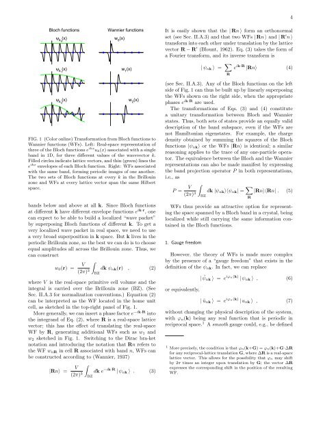
FIG. 1 (Color online) Transformation from Bloch <strong>functions</strong> to<br />
<strong>Wannier</strong> <strong>functions</strong> (WFs). Left: Real-space representation of<br />
three of the Bloch <strong>functions</strong> e ikx u k (x) associated with a single<br />
b<strong>and</strong> in 1D, for three different values of the wavevector k.<br />
Filled circles indicate lattice vectors, <strong>and</strong> thin (green) lines the<br />
e ikx envelopes of each Bloch function. Right: WFs associated<br />
with the same b<strong>and</strong>, forming periodic images of one another.<br />
The two sets of Bloch <strong>functions</strong> at every k in the Brillouin<br />
zone <strong>and</strong> WFs at every lattice vector span the same Hilbert<br />
space.<br />
b<strong>and</strong>s below <strong>and</strong> above at all k. Since Bloch <strong>functions</strong><br />
at different k have different envelope <strong>functions</strong> e ik·r , one<br />
can expect to be able to build a <strong>localized</strong> “wave packet”<br />
by superposing Bloch <strong>functions</strong> of different k. To get a<br />
very <strong>localized</strong> wave packet in real space, we need to use<br />
a very broad superposition in k space. But k lives in the<br />
periodic Brillouin zone, so the best we can do is to choose<br />
equal amplitudes all across the Brillouin zone. Thus, we<br />
can construct<br />
w 0 (r) =<br />
V<br />
(2π) 3 ∫BZ<br />
dk ψ nk (r) , (2)<br />
where V is the real-space primitive cell volume <strong>and</strong> the<br />
integral is carried over the Brillouin zone (BZ). (See<br />
Sec. II.A.3 for normalization conventions.) Equation (2)<br />
can be interpreted as the WF located in the home unit<br />
cell, as sketched in the top-right panel of Fig. 1.<br />
More generally, we can insert a phase factor e −ik·R into<br />
the integr<strong>and</strong> of Eq. (2), where R is a real-space lattice<br />
vector; this has the effect of translating the real-space<br />
WF by R, generating additional WFs such as w 1 <strong>and</strong><br />
w 2 sketched in Fig. 1. Switching to the Dirac bra-ket<br />
notation <strong>and</strong> introducing the notation that Rn refers to<br />
the WF w nR in cell R associated with b<strong>and</strong> n, WFs can<br />
be constructed according to (<strong>Wannier</strong>, 1937)<br />
|Rn⟩ =<br />
V<br />
(2π) 3 ∫BZ<br />
dk e −ik·R | ψ nk ⟩ . (3)<br />
(see Sec. II.A.3). Any of the Bloch <strong>functions</strong> on the left<br />
side of Fig. 1 can thus be built up by linearly superposing<br />
the WFs shown on the right side, when the appropriate<br />
phases e ik·R are used.<br />
The transformations of Eqs. (3) <strong>and</strong> (4) constitute<br />
a unitary transformation between Bloch <strong>and</strong> <strong>Wannier</strong><br />
states. Thus, both sets of states provide an equally valid<br />
description of the b<strong>and</strong> subspace, even if the WFs are<br />
not Hamiltonian eigenstates. For example, the charge<br />
density obtained by summing the squares of the Bloch<br />
<strong>functions</strong> |ψ nk ⟩ or the WFs |Rn⟩ is identical; a similar<br />
reasoning applies to the trace of any one-particle operator.<br />
The equivalence between the Bloch <strong>and</strong> the <strong>Wannier</strong><br />
representations can also be made manifest by expressing<br />
the b<strong>and</strong> projection operator P in both representations,<br />
i.e., as<br />
P =<br />
V<br />
(2π) 3 ∫BZ<br />
dk |ψ nk ⟩⟨ψ nk | = ∑ R<br />
|Rn⟩⟨Rn| . (5)<br />
WFs thus provide an attractive option for representing<br />
the space spanned by a Bloch b<strong>and</strong> in a crystal, being<br />
<strong>localized</strong> while still carrying the same information contained<br />
in the Bloch <strong>functions</strong>.<br />
1. Gauge freedom<br />
However, the theory of WFs is made more complex<br />
by the presence of a “gauge freedom” that exists in the<br />
definition of the ψ nk . In fact, we can replace<br />
or equivalently,<br />
| ˜ψ nk ⟩ = e iφn(k) | ψ nk ⟩ , (6)<br />
| ũ nk ⟩ = e iφ n(k) | u nk ⟩ , (7)<br />
without changing the physical description of the system,<br />
with φ n (k) being any real function that is periodic in<br />
reciprocal space. 1 A smooth gauge could, e.g., be defined<br />
1 More precisely, the condition is that φ n (k+G) = φ n (k)+G·∆R<br />
for any reciprocal-lattice translation G, where ∆R is a real-space<br />
lattice vector. This allows for the possibility that φ n may shift<br />
by 2π times an integer upon translation by G; the vector ∆R<br />
expresses the corresponding shift in the position of the resulting<br />
WF.


