Maximally localized Wannier functions: Theory and applications

54
Typically one chooses to solve for either the electric
field E nk
or the magnetic field H nk
. Once the Bloch
states for the periodic crystal are obtained, a basis of
magnetic or electric field Wannier functions may be constructed
using the usual definition, e.g., for the magnetic
field
W (H)
nR (r) =
V
(2π) 3 ∫BZ
dk e −ik·R ∑ m
U (k)
mnH mk (r), (145)
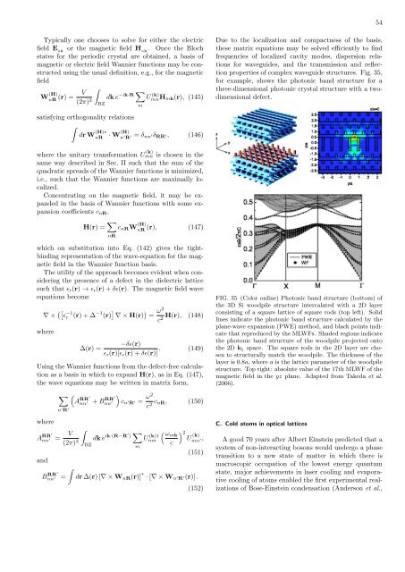
Due to the localization and compactness of the basis,
these matrix equations may be solved efficiently to find
frequencies of localized cavity modes, dispersion relations
for waveguides, and the transmission and reflection
properties of complex waveguide structures. Fig. 35,
for example, shows the photonic band structure for a
three-dimensional photonic crystal structure with a twodimensional
defect.
satisfying orthogonality relations
∫
dr W (H)∗
nR · W(H) n ′ R = δ ′ nn ′δ RR ′, (146)
where the unitary transformation U (k)
mn is chosen in the
same way described in Sec. II such that the sum of the
quadratic spreads of the Wannier functions is minimized,
i.e., such that the Wannier functions are maximally localized.
Concentrating on the magnetic field, it may be expanded
in the basis of Wannier functions with some expansion
coefficients c nR ,
H(r) = ∑ nR
c nR W (H)
nR
(r), (147)
which on substitution into Eq. (142) gives the tightbinding
representation of the wave-equation for the magnetic
field in the Wannier function basis.
The utility of the approach becomes evident when considering
the presence of a defect in the dielectric lattice
such that ϵ r (r) → ϵ r (r) + δϵ(r). The magnetic field wave
equations become
∇ × ([ ϵ −1
r
where
(r) + ∆ −1 (r) ] ∇ × H(r) ) = ω2
H(r), (148)
c2 ∆(r) =
−δϵ(r)
ϵ r (r)[ϵ r (r) + δϵ(r)] . (149)
Using the Wannier functions from the defect-free calculation
as a basis in which to expand H(r), as in Eq. (147),
the wave equations may be written in matrix form,
where
∑ (
)
A RR′
nn + ′ BRR′ nn c ′ n′ R ′ = ω2
c 2 c nR, (150)
n ′ R ′
A RR′
nn = V
′ (2π)
∫BZ
3 dk e ∑ ik·(R−R′ )
m
and
B RR′
nn ′
= ∫
U (k)†
nm
( ωmk
c
) 2
U
(k)
mn ′,
(151)
dr ∆(r) [∇ × W nR (r)] ∗ · [∇ × W n′ R ′(r)] .
(152)
FIG. 35 (Color online) Photonic band structure (bottom) of
the 3D Si woodpile structure intercalated with a 2D layer
consisting of a square lattice of square rods (top left). Solid
lines indicate the photonic band structure calculated by the
plane-wave expansion (PWE) method, and black points indicate
that reproduced by the MLWFs. Shaded regions indicate
the photonic band structure of the woodpile projected onto
the 2D k ∥ space. The square rods in the 2D layer are chosen
to structurally match the woodpile. The thickness of the
layer is 0.8a, where a is the lattice parameter of the woodpile
structure. Top right: absolute value of the 17th MLWF of the
magnetic field in the yz plane. Adapted from Takeda et al.
(2006).
C. Cold atoms in optical lattices
A good 70 years after Albert Einstein predicted that a
system of non-interacting bosons would undergo a phase
transition to a new state of matter in which there is
macroscopic occupation of the lowest energy quantum
state, major achievements in laser cooling and evaporative
cooling of atoms enabled the first experimental realizations
of Bose-Einstein condensation (Anderson et al.,