Maximally localized Wannier functions: Theory and applications

14
Energy (eV)
10
5
0
-5
-10
-15
-20
Γ M K Γ
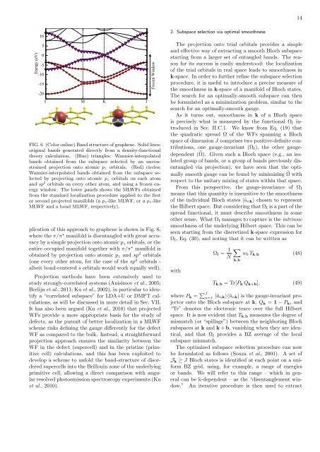
FIG. 6 (Color online) Band structure of graphene. Solid lines:
original bands generated directly from a density-functional
theory calculation. (Blue) triangles: Wannier-interpolated
bands obtained from the subspace selected by an unconstrained
projection onto atomic p z orbitals. (Red) circles:
Wannier-interpolated bands obtained from the subspace selected
by projecting onto atomic p z orbitals on each atom
and sp 2 orbitals on every other atom, and using a frozen energy
window. The lower panels shows the MLWFs obtained
from the standard localization procedure applied to the first
or second projected manifolds (a p z -like MLWF, or a p z -like
MLWF and a bond MLWF, respectively).
plication of this approach to graphene is shown in Fig. 6,
where the π/π ⋆ manifold is disentangled with great accuracy
by a simple projection onto atomic p z orbitals, or the
entire occupied manifold together with π/π ⋆ manifold is
obtained by projection onto atomic p z and sp 2 orbitals
(one every other atom, for the case of the sp 2 orbitals -
albeit bond-centered s orbitals would work equally well).
Projection methods have been extensively used to
study strongly-correlated systems (Anisimov et al., 2005;
Berlijn et al., 2011; Ku et al., 2002), in particular to identify
a “correlated subspace” for LDA+U or DMFT calculations,
as will be discussed in more detail in Sec. VII.
It has also been argued (Ku et al., 2010) that projected
WFs provide a more appropriate basis for the study of
defects, as the pursuit of better localization in a MLWF
scheme risks defining the gauge differently for the defect
WF as compared to the bulk. Instead, a straightforward
projection approach ensures the similarity between the
WF in the defect (supercell) and in the pristine (primitive
cell) calculations, and this has been exploited to
develop a scheme to unfold the band-structure of disordered
supercells into the Brillouin zone of the underlying
primitive cell, allowing a direct comparison with angular
resolved photoemission spectroscopy experiments (Ku
et al., 2010).
Frozen Window
2. Subspace selection via optimal smoothness
The projection onto trial orbitals provides a simple
and effective way of extracting a smooth Bloch subspace
starting from a larger set of entangled bands. The reason
for its success is easily understood: the localization
of the trial orbitals in real space leads to smoothness in
k-space. In order to further refine the subspace selection
procedure, it is useful to introduce a precise measure of
the smoothness in k-space of a manifold of Bloch states.
The search for an optimally-smooth subspace can then
be formulated as a minimization problem, similar to the
search for an optimally-smooth gauge.
As it turns out, smoothness in k of a Bloch space
is precisely what is measured by the functional Ω I introduced
in Sec. II.C.1. We know from Eq. (19) that
the quadratic spread Ω of the WFs spanning a Bloch
space of dimension J comprises two positive-definite contributions,
one gauge-invariant (Ω I ), the other gaugedependent
(˜Ω). Given such a Bloch space (e.g., an isolated
group of bands, or a group of bands previously disentangled
via projection), we have seen that the optimally
smooth gauge can be found by minimizing ˜Ω with
respect to the unitary mixing of states within that space.
From this perspective, the gauge-invariance of Ω I
means that this quantity is insensitive to the smoothness
of the individual Bloch states |ũ nk ⟩ chosen to represent
the Hilbert space. But considering that Ω I is a part of the
spread functional, it must describe smoothness in some
other sense. What Ω I manages to capture is the intrinsic
smoothness of the underlying Hilbert space. This can be
seen starting from the discretized k-space expression for
Ω I , Eq. (30), and noting that it can be written as
with
Ω I = 1 ∑
w b T k,b (48)
N
k,b
T k,b = Tr[P k Q k+b ], (49)
where P k = ∑ J
n=1 |ũ nk⟩⟨ũ nk | is the gauge-invariant projector
onto the Bloch subspace at k, Q k = 1 − P k , and
“Tr” denotes the electronic trace over the full Hilbert
space. It is now evident that T k,b measures the degree of
mismatch (or “spillage”) between the neighboring Bloch
subspaces at k and k + b, vanishing when they are identical,
and that Ω I provides a BZ average of the local
subspace mismatch.
The optimized subspace selection procedure can now
be formulated as follows (Souza et al., 2001). A set of
J k ≥ J Bloch states is identified at each point on a uniform
BZ grid, using, for example, a range of energies
or bands. We will refer to this range – which in general
can be k-dependent – as the “disentanglement window.”
An iterative procedure is then used to extract