

Maximally localized Wannier functions: Theory and applications
Maximally localized Wannier functions: Theory and applications
Maximally localized Wannier functions: Theory and applications

Create successful ePaper yourself
Turn your PDF publications into a flip-book with our unique Google optimized e-Paper software.
42<br />
<strong>Wannier</strong>-interpolated first-principles b<strong>and</strong>s was carried<br />
out by Liu et al. (2009). This formalism is not restricted<br />
to cubic crystals, <strong>and</strong> the authors used it to calculate the<br />
Hall conductivity of hcp Mg (Liu et al., 2009) <strong>and</strong> the<br />
magnetoconductivity of MgB 2 (Yang et al., 2008).<br />
<strong>Wannier</strong> interpolation has also been used to determine<br />
the Seebeck coefficient in hole-doped LaRhO 3<br />
<strong>and</strong> CuRhO 2 (Usui et al., 2009), in electron-doped<br />
SrTiO 3 (Usui et al., 2010), in SiGe nanowires (Shelley<br />
<strong>and</strong> Mostofi, 2011), <strong>and</strong> in ternary skutterudites (Volja<br />
et al., 2011).<br />
Energy (Ry)<br />
(k) (atomic units)<br />
-Ω tot<br />
xy<br />
0.80<br />
0.78<br />
0.76<br />
0.74<br />
0.72<br />
0.70<br />
4000<br />
2000<br />
0<br />
ε F<br />
C. Berry curvature <strong>and</strong> anomalous Hall conductivity<br />
The velocity matrix elements between Bloch eigenstates<br />
take the form (Blount, 1962)<br />
⟨ψ nk |ħv α |ψ mk ⟩ = δ nm ∂ α ϵ nk − i(ϵ mk − ϵ nk ) [A k,α ] nm<br />
,<br />
(108)<br />
where<br />
[A k,α ] nm<br />
= i⟨u nk |∂ α u mk ⟩ (109)<br />
is the matrix generalization of the Berry connection of<br />
Eq. (95).<br />
In the examples discussed in the previous section the<br />
static transport coefficients could be calculated from the<br />
first term in Eq. (108), the intrab<strong>and</strong> velocity. The second<br />
term describes vertical interb<strong>and</strong> transitions, which<br />
dominate the optical spectrum of crystals over a wide<br />
frequency range. Interestingly, under certain conditions,<br />
virtual interb<strong>and</strong> transitions also contribute to the dc<br />
Hall conductivity. This so-called anomalous Hall effect<br />
occurs in ferromagnets from the combination of exchange<br />
splitting <strong>and</strong> spin-orbit interaction. For a recent review,<br />
see Nagaosa et al. (2010).<br />
In the same way that WFs proved helpful for evaluating<br />
∂ k ϵ nk , they can be useful for calculating quantities<br />
containing k-derivatives of the cell-periodic Bloch states,<br />
such as the Berry connection of Eq. (109). A number of<br />
properties are naturally expressed in this form. In addition<br />
to the interb<strong>and</strong> optical conductivity <strong>and</strong> the anomalous<br />
Hall conductivity (AHC), other examples include the<br />
electric polarization (Sec. V.A) as well as the orbital magnetization<br />
<strong>and</strong> magnetoelectric coupling (Sec. V.C).<br />
Let us focus on the Berry curvature F nk [Eq. (96)], a<br />
quantity with profound effects on the dynamics of electrons<br />
in crystals (Xiao et al., 2010). F nk can be nonzero<br />
if either spatial inversion or time-reversal symmetries are<br />
broken in the crystal, <strong>and</strong> when present acts as a kind<br />
of “magnetic field” in k-space, with the Berry connection<br />
A nk playing the role of the vector potential. This<br />
effective field gives rise to a Hall effect in ferromagnets<br />
even in the absence of an actual applied B-field (hence<br />
Γ<br />
H<br />
P<br />
N<br />
Γ<br />
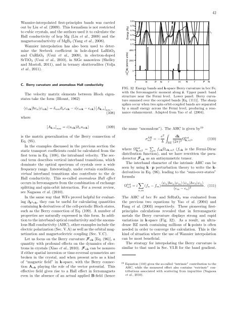
FIG. 32 Energy b<strong>and</strong>s <strong>and</strong> k-space Berry curvature in bcc Fe,<br />
with the ferromagnetic moment along ẑ. Upper panel: b<strong>and</strong><br />
structure near the Fermi level. Lower panel: Berry curvature<br />
summed over the occupied b<strong>and</strong>s [Eq. (111)]. The sharp<br />
spikes occur when two spin-orbit-coupled b<strong>and</strong>s are separated<br />
by a small energy across the Fermi level, producing a resonance<br />
enhancement. Adapted from Yao et al. (2004).<br />
the name “anomalous”). The AHC is given by 19<br />
σ AH<br />
αβ<br />
= − e2<br />
ħ<br />
∫<br />
BZ<br />
H<br />
N<br />
Γ<br />
dk<br />
(2π) 3 Ωtot k,αβ, (110)<br />
where Ω tot<br />
k,αβ = ∑ n f nkΩ nk,αβ (f nk is the Fermi-Dirac<br />
distribution function), <strong>and</strong> we have rewritten the pseudovector<br />
F nk as an antisymmetric tensor.<br />
The interb<strong>and</strong> character of the intrinsic AHC can be<br />
seen by using k · p perturbation theory to write the k-<br />
derivatives in Eq. (96), leading to the “sum-over-states”<br />
formula<br />
Ω tot<br />
αβ = i ∑ (f n − f m ) ⟨ψ n|ħv α |ψ m ⟩⟨ψ m |ħv β |ψ n ⟩<br />
(ϵ<br />
n,m<br />
m − ϵ n ) 2 . (111)<br />
The AHC of bcc Fe <strong>and</strong> SrRuO 3 was evaluated from<br />
the previous two equations by Yao et al. (2004) <strong>and</strong><br />
Fang et al. (2003) respectively. These pioneering firstprinciples<br />
calculations revealed that in ferromagnetic<br />
metals the Berry curvature displays strong <strong>and</strong> rapid<br />
variations in k-space (Fig. 32). As a result, an ultradense<br />
BZ mesh containing millions of k-points is often<br />
needed in order to converge the calculation. This is the<br />
kind of situation where the use of <strong>Wannier</strong> interpolation<br />
can be most beneficial.<br />
The strategy for interpolating the Berry curvature is<br />
similar to that used in Sec. VI.B for the b<strong>and</strong> gradient.<br />
19 Equation (110) gives the so-called “intrinsic” contribution to the<br />
AHC, while the measured effect also contains “extrinsic” contributions<br />
associated with scattering from impurities (Nagaosa<br />
et al., 2010).<br />
P<br />
N


