Maximally localized Wannier functions: Theory and applications

More documents

Recommendations

Info

18 (LMOs) ϕ i (r) can be expressed as linear combinations of a set of molecular eigenstates ψ i (r) (the “canonical” MOs), typically chosen to be the occupied ones, ϕ i (r) = J∑ U ji ψ j (r). (56) j=1 The choice of gauge then arises from minimizing or maximizing some appropriate functional of the LMOs with respect to the coefficients U ij , under the constraint that the transformation (56) is unitary, which ensures the orthonormality of the resulting LMOs. The Foster-Boys criterion (FB) (Boys, 1960, 1966; Foster and Boys, 1960a). This is essentially the same as the Marzari-Vanderbilt criterion of minimizing the sum of the quadratic spreads, except that the sum runs over the orbitals in the molecule, rather than in one crystal cell, Ω FB = J∑ [⟨ϕ i |r 2 |ϕ i ⟩ − ⟨ϕ i |r|ϕ i ⟩ 2 ]. (57) i=1 Interestingly, this criterion is equivalent to minimizing the “self-extension” of the orbitals (Boys, 1966), J∑ ∫ dr 1 dr 2 |ϕ i (r 1 )| 2 (r 1 − r 2 ) 2 |ϕ i (r 1 )| 2 (58) i=1 and also to maximizing the sum of the squares of the distance between the charge centers of the orbitals J∑ |⟨ϕ i |r|ϕ i ⟩ − ⟨ϕ j |r|ϕ j ⟩| 2 , (59) i,j=1 which is closely related to Eq. (44) of Sec. II.F.2. The relation between Eqs. (57)–(59) is discussed in Boys (1966). The Edmiston-Ruedenberg criterion (ER). Here localization is achieved by maximizing the Coulomb selfinteraction of the orbitals (Edmiston and Ruedenberg, 1963) Ω ER = J∑ ∫ dr 1 dr 2 |ϕ i (r 1 )| 2 (r 1 − r 2 ) −1 |ϕ i (r 2 )| 2 . (60) i=1 From a computational point of view, the ER approach is more demanding (it scales as J 4 versus J 2 for FB), but recently more efficient implementations have been developed (Subotnik et al., 2007). The von Niessen criterion (VN). The goal here is to maximize the density overlap of the orbitals (von Niessen, 1972) Ω VN = J∑ ∫ dr 1 dr 2 |ϕ i (r 1 )| 2 δ(r 1 − r 2 )|ϕ i (r 2 )| 2 . (61) i=1 The Pipek-Mezey criterion (Pipek and Mezey, 1989) (PM). This approach differs from the ones above in that it makes reference to some extrinsic objects. The idea is to maximize the sum of the squares of the Mulliken atomic charges (Mulliken, 1955). These are obtained with respect to a set of atomic orbitals χ µ centered on atomic sites A. We define P A = ∑ ∑ D µν S µν (62) µ∈A ν where the sum over µ involves all of the atomic states on atom site A, D µν is the density matrix in the atomic basis, and S µν = ⟨χ µ |χ ν ⟩ is the overlap operator. The functional to be maximized is given by Ω PM = J∑ ∑N A i=1 A=1 |⟨ϕ i |P A |ϕ i ⟩| 2 . (63) This is somewhat similar in spirit to the projection scheme discussed in Sec. II.B, except that it is not a one-shot procedure. As indicated in Eq. (56), all of these schemes amount to unitary transformations among the canonical MOs and, as such, they give rise to representations of the electronic structure of the system that are equivalent to that provided by the original set of eigenstates. For the purpose of providing chemical intuition, the usefulness of a given scheme depends on how well it matches a particular viewpoint of bonding. There have been few studies of the VN scheme, but the FB, ER, and PM schemes have been extensively compared. In many cases all three approaches lead to similar localized orbitals which agree with the simple Lewis picture of bonding. A notable exception is for systems that exhibit both σ and π bonding. For a double bond, both the FB and ER schemes mix the σ and π orbitals, giving rise to two bent “banana bond” (or τ) orbitals (Pauling, 1960) as shown in Fig 10. When applied to benzene, both schemes give alternating σ and τ orbitals. Trivially, there are two equivalent sets of these orbitals, reminiscent of the two Kekulé structures for benzene. In contrast to the FB and ER schemes, PM provides a clear separation of σ and π orbitals. For example, in benzene PM gives a framework of six σ orbitals and three π orbitals around the ring. In some situations the FB and ER orbitals have been found to be quite different. This has been observed when the bonding in a molecule can be represented as two distinct resonant structures. The ER scheme generally gives orbitals corresponding to one of the possible structures, whilst the FB orbitals correspond a hybrid of the structures. An extreme example is CO 2 (Brown et al., 1977). In agreement with the O=C=O Lewis picture, ER gives two lone pairs on each oxygen and two τ orbitals between each carbon and oxygen. In contrast, the FB scheme gives a single lone pair on each oxygen and three highly polarized τ orbitals between the carbon and each oxygen, as shown in Fig. 10.
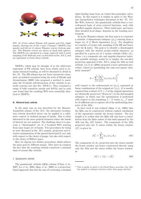
19 FIG. 10 (Color online) Ethane (left panels) and CO 2 (right panels), showing one of the τ-type (“banana”) MLWFs (top panels) and full set of valence Wannier centers (bottom panels). The Wannier centers are shown as small dark spheres. The MLWFs are calculated in a large supercell with Γ-point sampling of the Brillouin zone, as described in Sec. II.F.2, and are equivalent to Foster-Boys orbitals. MLWFs, which may be thought of as the solid-state equivalent of FB orbitals, have been widely used to examine chemical bonding, as will be discussed in detail in Sec. IV. The ER scheme has not been extensively examined, an isolated exception being the work of Miyake and Aryasetiawan (2008) who proposed a method to maximize the Coulomb self-interaction of the orbitals in periodic systems (see also Sec. VII.B.1). They examined a range of bulk transition metals and SrVO 3 and in each case found that the resulting WFs were essentially identical to MLWFs. B. Minimal-basis orbitals In the same way as was described for the Marzari- Vanderbilt scheme of Sec. II.C, the alternative localization criteria described above can be applied in a solidstate context to isolated groups of bands. One is often interested in the more general situation where the bands of interest are not isolated. The challenge then is to generate a “disentangled” set of J localized WFs starting from some larger set of bands. Two procedures for doing so were discussed in Sec. II.I, namely, projection and iterative minimization of the spread functional Ω, not only with respect to the choice of gauge, but also with respect to the choice of Hilbert space. Here we discuss two further procedures which achieve the same goal by different means. They have in common the fact that the resulting orbitals constitute a minimal basis of atomic-like orbitals. 1. Quasiatomic orbitals The quasiatomic orbitals (QOs) scheme (Chan et al., 2007; Lu et al., 2004; Qian et al., 2008) is a projectionbased approach that has the aim of extracting a minimal tight-binding basis from an initial first-principles calculation. In this regard it is similar in spirit to the Wannier interpolation techniques discussion in Sec. VI. Unlike WFs, however, the quasiatomic orbitals form a nonorthogonal basis of atom-centered functions, each with specified angular character. Their radial part, and hence their detailed local shape, depends on the bonding environment. As in the Wannier scheme, the first step is to construct a suitable J-dimensional subspace {ϕ n } starting from a larger set of J Bloch eigenstates {ψ n }. For simplicity we consider a Γ-point only sampling of the BZ and hence omit the k index. The goal is to identify a disentangled subspace with the desired atomic-orbital character, as specified by a given set of J atomic orbitals (AOs) |A i ⟩, where i is a composite site and angular-character index. One possible strategy would be to employ the one-shot projection approach of Sec. II.I.1, using the AOs as trial orbitals. Lu et al. (2004) proposed a more optimized procedure, based on maximizing the sum-over-square similarity measure 8 2 J∑ J∑ L = |ϕ ∣∣ n ⟩⟨ϕ n |A i ⟩ (64) ∣∣ i=1 n=1 with respect to the orthonormal set {ϕ n }, expressed as linear combinations of the original set {ψ n }. It is usually required that a subset of N ≤ J of the original eigenstates are identically preserved (“frozen in”) in the disentangled subspace, in which case the optimization is performed with respect to the remaining J − N states ϕ n . J must be of sufficient size to capture all of the antibonding character of the AOs. In later work it was realized (Qian et al., 2008) that the QOs can be constructed without explicit calculation of the eigenstates outside the frozen window. The key insight is to realize that the QOs will only have a contribution from the finite subset of this basis spanned by the AOs (see Eq. (67) below). The component of the AOs projected onto the N states within the frozen window |A ∥ i ⟩ is given by N |A ∥ i ⟩ = ∑ |ψ n ⟩⟨ψ n |A i ⟩. (65) n=1 The component of |A i ⟩ projected onto the states outside the frozen window can hence constructed directly using only the AOs and the states within the frozen window, as |A ⊥ i ⟩ = |A i ⟩ − |A ∥ i ⟩. (66) 8 This is similar in spirit to the Pipek-Mazey procedure, Eq. (62), but applied to subspace selection rather than gauge selection.
Page 1 and 2: Maximally localized Wannier functio
Page 3 and 4: 3 tition into separate “bands”,
Page 5 and 6: 5 such that ∇ k |u nk ⟩ is well
Page 7 and 8: 7 orbitals g n (r) corresponding to
Page 9 and 10: 9 to write down many alternative fi
Page 11 and 12: 11 To proceed further, we write dΩ
Page 13 and 14: 13 of the states in this larger man
Page 15 and 16: 15 self-consistently at each k-poin
Page 17: 17 Problems associated with reachin
Page 21 and 22: 21 Energy (eV) -10 -15 Carbon s-orb
Page 23 and 24: 23 density operator in an LCAO basi
Page 25 and 26: 25 15 Energy (eV) 10 5 0 -5 Frozen
Page 27 and 28: 27 FIG. 19 (Color online) Contour-s
Page 29 and 30: 29 straightforward. The electric di
Page 31 and 32: 31 localization length near an insu
Page 33 and 34: 33 Giustino et al. (2003) and used
Page 35 and 36: 35 which is the desired k-space bul
Page 37 and 38: 37 FIG. 25 (Color online) Schematic
Page 39 and 40: 39 obtained by unfolding the Γ-poi
Page 41 and 42: 41 FIG. 31 (Color online) Surface d
Page 43 and 44: 43 One first evaluates certain obje
Page 45 and 46: 45 VII. WANNIER FUNCTIONS AS BASIS
Page 47 and 48: 47 the conductor to the leads (Datt
Page 49 and 50: 49 operators that are represented i
Page 51 and 52: 51 2. Self-interaction and DFT + Hu
Page 53 and 54: may be expressed as where c = (µ 0
Page 55 and 56: 55 1995; Bradley et al., 1995; Davi
Page 57 and 58: 57 Alfimov, G. L., P. G. Kevrekidis
Page 59 and 60: 59 Franchini, C., R. Kovacik, M. Ma
Page 61 and 62: 61 sity Press, Cambridge). Marzari,
Page 63 and 64: 63 Silvestrelli, P. L., and M. Parr

Maximally localized Wannier functions: Theory and applications

You also want an ePaper? Increase the reach of your titles

Delete template?

Save as template?