Maximally localized Wannier functions: Theory and applications

31
localization length near an insulator-to-metal transition
in 1D and 2D model systems was studied using quantum
Monte Carlo methods by Hine and Foulkes (2007).
Finally, the concept of electric enthalpy was generalized
to the many-body case by Umari et al. (2005), allowing
to calculate for the first time dielectric properties
with quantum Monte Carlo, and applied to the case of
the polarizabilities (Umari et al., 2005) and hyperpolarizabilities
(Umari and Marzari, 2009) of periodic hydrogen
chains.
B. Local polar properties and dielectric response
Is Sec.V.A.1 we emphasized the equivalence of the k-
space Berry-phase expression for the electric polarization,
Eq. (90), and the expression written in terms of the locations
of the Wannier centers r n , Eq. (89). The latter
has the advantage of being a real-space expression,
thereby opening up opportunities for localized descriptions
and decompositions of polar properties and dielectric
responses. We emphasize again that MLWFs have
no privileged role in Eq. (89); the expression remains
correct for any WFs that are sufficiently well localized
that the centers r n are well defined. Nevertheless, one
may argue heuristically that MLWFs provide the most
natural local real-space description of dipolar properties
in crystals and other condensed phases.
1. Polar properties and dynamical charges of crystals
Many dielectric properties of crystalline solids are most
easily computed directly in the k-space Bloch representation.
Even before it was understood how to compute the
polarization P via the Berry-phase theory of Eq. (90), it
was well known how to compute derivatives of P using
linear-response methods (Baroni et al., 2001; de Gironcoli
et al., 1989; Resta, 1992). Useful derivatives include the
electric susceptibility χ ij = dP i /dE j and the Born (or
dynamical) effective charges Zi,τj ∗ = V dP i/dR τj , where i
and j are Cartesian labels and R τj is the displacement of
sublattice τ in direction j. With the development of the
Berry-phase theory, it also became possible to compute
effective charges by finite differences. Similarly, with the
electric-enthalpy approach of Eq. (91) it became possible
to compute electric susceptibilities by finite differences as
well (Souza et al., 2002; Umari and Pasquarello, 2002).
The Wannier representation provides an alternative
method for computing such dielectric quantities by finite
differences. One computes the derivatives dr n,i /dE j
or dr n,i /dR τj of the Wannier centers by finite differences,
then sums these to get the desired χ ij or Zi,τj ∗ . An example
of such a calculation for Z ∗ in GaAs was presented
already in Sec. VII of Marzari and Vanderbilt (1997),
and an application of the Wannier approach of Nunes
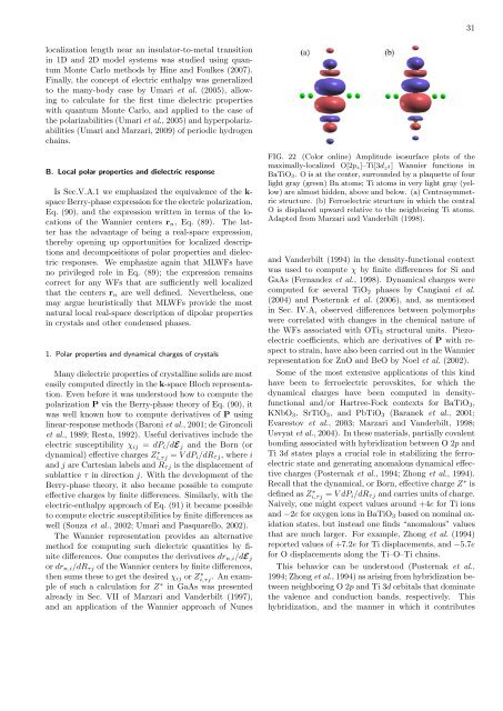
FIG. 22 (Color online) Amplitude isosurface plots of the
maximally-localized O[2p z ]–Ti[3d z 2] Wannier functions in
BaTiO 3 . O is at the center, surrounded by a plaquette of four
light gray (green) Ba atoms; Ti atoms in very light gray (yellow)
are almost hidden, above and below. (a) Centrosymmetric
structure. (b) Ferroelectric structure in which the central
O is displaced upward relative to the neighboring Ti atoms.
Adapted from Marzari and Vanderbilt (1998).
and Vanderbilt (1994) in the density-functional context
was used to compute χ by finite differences for Si and
GaAs (Fernandez et al., 1998). Dynamical charges were
computed for several TiO 2 phases by Cangiani et al.
(2004) and Posternak et al. (2006), and, as mentioned
in Sec. IV.A, observed differences between polymorphs
were correlated with changes in the chemical nature of
the WFs associated with OTi 3 structural units. Piezoelectric
coefficients, which are derivatives of P with respect
to strain, have also been carried out in the Wannier
representation for ZnO and BeO by Noel et al. (2002).
Some of the most extensive applications of this kind
have been to ferroelectric perovskites, for which the
dynamical charges have been computed in densityfunctional
and/or Hartree-Fock contexts for BaTiO 3 ,
KNbO 3 , SrTiO 3 , and PbTiO 3 (Baranek et al., 2001;
Evarestov et al., 2003; Marzari and Vanderbilt, 1998;
Usvyat et al., 2004). In these materials, partially covalent
bonding associated with hybridization between O 2p and
Ti 3d states plays a crucial role in stabilizing the ferroelectric
state and generating anomalous dynamical effective
charges (Posternak et al., 1994; Zhong et al., 1994).
Recall that the dynamical, or Born, effective charge Z ∗ is
defined as Zi,τj ∗ = V dP i/dR τj and carries units of charge.
Naively, one might expect values around +4e for Ti ions
and −2e for oxygen ions in BaTiO 3 based on nominal oxidation
states, but instead one finds “anomalous” values
that are much larger. For example, Zhong et al. (1994)
reported values of +7.2e for Ti displacements, and −5.7e
for O displacements along the Ti–O–Ti chains.
This behavior can be understood (Posternak et al.,
1994; Zhong et al., 1994) as arising from hybridization between
neighboring O 2p and Ti 3d orbitals that dominate
the valence and conduction bands, respectively. This
hybridization, and the manner in which it contributes