Maximally localized Wannier functions: Theory and applications

41
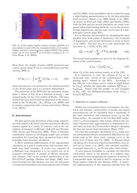
FIG. 31 (Color online) Surface density-of-states (SDOS) of a
semi-infinite crystal of Sb 2 Te 3 terminated with a [111] surface.
Lighter (warmer) colors represent a higher SDOS. The surface
states can be seen around Γ as (red) lines crossing at E = 0.
From Zhang et al. (2009a).
From these, the density of states (DOS) projected onto
a given atomic plane P can be obtained(Grosso and Parravicini,
2000) as
N P l
(k ∥ , ϵ) = − 1 π Im ∑ n∈P
G nn
ll (k ∥ , ϵ + iη), (105)
where the sum over n is restricted to the orbitals ascribed
to the chosen plane and η is a positive infinitesimal.
The projection of the DOS onto the outermost atomic
plane is shown in Fig. 31 as a function of energy ϵ and
momentum k ∥ for the (111) surface of Sb 2 Te 3 . The same
method has been used to find the dispersion of the surface
bands in the TI alloy Bi 1−x Sb x (Zhang et al., 2009b) and
in ternary compounds with a honeycomb lattice (Zhang
et al., 2011b).
B. Band derivatives
The first and second derivatives of the energy eigenvalues
with respect to k (band velocities and inverse effective
masses) appear in a variety of contexts, such as the calculation
of transport coefficients (Ashcroft and Mermin,
1976; Grosso and Parravicini, 2000). There is therefore
considerable interest in developing simple and accurate
procedures for extracting these parameters from a firstprinciples
band structure calculation.
A direct numerical differentiation of the eigenenergies
calculated on a grid is cumbersome and becomes unreliable
near band crossings. It is also very expensive if
a Brillouin zone integration is to be carried out, as in
transport calculations. A number of efficient interpolation
schemes, such as the method implemented in the
BoltzTraP package (Madsen and Singh, 2006), have
been developed for this purpose, but they are still prone
to numerical instabilities near band degeneracies (Uehara
and Tse, 2000). Such instabilities can be avoided by using
a tight-binding parametrization to fit the first-principles
band structure (Mazin et al., 2000; Schulz et al., 1992).
As shown by Graf and Vogl (1992) and Boykin (1995),
both the first and the second derivatives are easily computed
within tight-binding methods, even in the presence
of band degeneracies, and the same can be done in a firstprinciples
context using WFs.
Let us illustrate the procedure by calculating the band
gradient away from points of degeneracy; the treatment
of degeneracies and second derivatives is given in Yates
et al. (2007). The first step is to take analytically the
derivative ∂ α = ∂/∂k α of Eq. (98),
H W k,α ≡ ∂ α H W k
= ∑ R
e ik·R iR α ⟨0|H|R⟩. (106)
The actual band gradients are given by the diagonal elements
of the rotated matrix,
]
∂ α ϵ nk =
[U † k HW k,αU k (107)
where U k is the same unitary matrix as in Eq. (99).
It is instructive to view the columns of U k as orthonormal
state vectors in the J-dimensional “tightbinding
space” defined by the WFs. According to
Eq. (99) the n-th column vector, which we shall denote
by ||ϕ nk ⟩⟩, satisfies the eigenvalue equation Hk W||ϕ nk⟩⟩ =
ϵ nk ||ϕ nk ⟩⟩. Armed with this insight, we now recognize
in Eq. (107) the Hellmann-Feynman result ∂ α ϵ nk =
⟨⟨ϕ nk ||∂ α Hk W||ϕ nk⟩⟩.
1. Application to transport coefficients
Within the semiclassical theory of transport, the electrical
and thermal conductivities of metals and doped
semiconductors can be calculated from a knowledge of
the band derivatives and relaxation times τ nk on the
Fermi surface. An example is the low-field Hall conductivity
σ xy of non-magnetic cubic metals, which in the constant
relaxation-time approximation is independent of τ
and takes the form of a Fermi-surface integral containing
the first and second band derivatives (Hurd, 1972).
Previous first-principles calculations of σ xy using various
interpolation schemes encountered difficulties for materials
such as Pd, where band crossings occur at the
Fermi level (Uehara and Tse, 2000). A Wannier-based
calculation free from such numerical instabilities was carried
out by Yates et al. (2007), who obtained carefullyconverged
values for σ xy in Pd and other cubic metals.
A more general formalism to calculate the electrical
conductivity tensor in the presence of a uniform magnetic
field involves integrating the equations of motion of
a wavepacket under the field to find its trajectory on the
Fermi surface (Ashcroft and Mermin, 1976). A numerical
implementation of this approach starting from the
nn