Maximally localized Wannier functions: Theory and applications

More documents

Recommendations

Info

14 Energy (eV) 10 5 0 -5 -10 -15 -20 Γ M K Γ FIG. 6 (Color online) Band structure of graphene. Solid lines: original bands generated directly from a density-functional theory calculation. (Blue) triangles: Wannier-interpolated bands obtained from the subspace selected by an unconstrained projection onto atomic p z orbitals. (Red) circles: Wannier-interpolated bands obtained from the subspace selected by projecting onto atomic p z orbitals on each atom and sp 2 orbitals on every other atom, and using a frozen energy window. The lower panels shows the MLWFs obtained from the standard localization procedure applied to the first or second projected manifolds (a p z -like MLWF, or a p z -like MLWF and a bond MLWF, respectively). plication of this approach to graphene is shown in Fig. 6, where the π/π ⋆ manifold is disentangled with great accuracy by a simple projection onto atomic p z orbitals, or the entire occupied manifold together with π/π ⋆ manifold is obtained by projection onto atomic p z and sp 2 orbitals (one every other atom, for the case of the sp 2 orbitals - albeit bond-centered s orbitals would work equally well). Projection methods have been extensively used to study strongly-correlated systems (Anisimov et al., 2005; Berlijn et al., 2011; Ku et al., 2002), in particular to identify a “correlated subspace” for LDA+U or DMFT calculations, as will be discussed in more detail in Sec. VII. It has also been argued (Ku et al., 2010) that projected WFs provide a more appropriate basis for the study of defects, as the pursuit of better localization in a MLWF scheme risks defining the gauge differently for the defect WF as compared to the bulk. Instead, a straightforward projection approach ensures the similarity between the WF in the defect (supercell) and in the pristine (primitive cell) calculations, and this has been exploited to develop a scheme to unfold the band-structure of disordered supercells into the Brillouin zone of the underlying primitive cell, allowing a direct comparison with angular resolved photoemission spectroscopy experiments (Ku et al., 2010). Frozen Window 2. Subspace selection via optimal smoothness The projection onto trial orbitals provides a simple and effective way of extracting a smooth Bloch subspace starting from a larger set of entangled bands. The reason for its success is easily understood: the localization of the trial orbitals in real space leads to smoothness in k-space. In order to further refine the subspace selection procedure, it is useful to introduce a precise measure of the smoothness in k-space of a manifold of Bloch states. The search for an optimally-smooth subspace can then be formulated as a minimization problem, similar to the search for an optimally-smooth gauge. As it turns out, smoothness in k of a Bloch space is precisely what is measured by the functional Ω I introduced in Sec. II.C.1. We know from Eq. (19) that the quadratic spread Ω of the WFs spanning a Bloch space of dimension J comprises two positive-definite contributions, one gauge-invariant (Ω I ), the other gaugedependent (˜Ω). Given such a Bloch space (e.g., an isolated group of bands, or a group of bands previously disentangled via projection), we have seen that the optimally smooth gauge can be found by minimizing ˜Ω with respect to the unitary mixing of states within that space. From this perspective, the gauge-invariance of Ω I means that this quantity is insensitive to the smoothness of the individual Bloch states |ũ nk ⟩ chosen to represent the Hilbert space. But considering that Ω I is a part of the spread functional, it must describe smoothness in some other sense. What Ω I manages to capture is the intrinsic smoothness of the underlying Hilbert space. This can be seen starting from the discretized k-space expression for Ω I , Eq. (30), and noting that it can be written as with Ω I = 1 ∑ w b T k,b (48) N k,b T k,b = Tr[P k Q k+b ], (49) where P k = ∑ J n=1 |ũ nk⟩⟨ũ nk | is the gauge-invariant projector onto the Bloch subspace at k, Q k = 1 − P k , and “Tr” denotes the electronic trace over the full Hilbert space. It is now evident that T k,b measures the degree of mismatch (or “spillage”) between the neighboring Bloch subspaces at k and k + b, vanishing when they are identical, and that Ω I provides a BZ average of the local subspace mismatch. The optimized subspace selection procedure can now be formulated as follows (Souza et al., 2001). A set of J k ≥ J Bloch states is identified at each point on a uniform BZ grid, using, for example, a range of energies or bands. We will refer to this range – which in general can be k-dependent – as the “disentanglement window.” An iterative procedure is then used to extract
15 self-consistently at each k-point the J-dimensional subspace that, when integrated across the BZ, will give the smallest possible value of Ω I . Viewed as function of k, the Bloch subspace obtained at the end of this iterative minimization is “optimally smooth” in that it changes as little as possible with k. Typically the minimization starts from an initial guess for the target subspace given, e.g., by projection onto trial orbitals. The algorithm is also easily modified to preserve identically a chosen subset of the Bloch eigenstates inside the disentanglement window, e.g., those spanning a narrower range of energies or bands; we refer to these as comprising a “frozen energy window.” As in the case of the one-shot projection, the outcome of this iterative procedure is a set of J Bloch-like states at each k which are linear combinations of the initial J k eigenstates. One important difference is that the resulting states are not guaranteed to be individually smooth, and the minimization of Ω I must therefore be followed by a gauge-selection step, which is in every way identical to the one described earlier for isolated groups of bands. Alternatively, it is possible to combine the two steps, and minimize Ω = Ω I + ˜Ω simultaneously with respect to the choice of Hilbert subspace and the choice of gauge (Thygesen et al., 2005a,b); this should lead to the most-localized set of J WFs that can be constructed from the initial J k Bloch states. In all three cases, the entire process amounts to a linear transformation taking from J k initial eigenstates to J smooth Bloch-like states, | ˜ψ nk ⟩ = ∑J k m=1 |ψ mk ⟩V k,mn . (50) In the case of the projection procedure, the explicit expression for the J k × J matrix V k can be surmised from Eqs. (46) and (47). Let us compare the one-shot projection and iterative procedures for subspace selection, using crystalline copper as an example. Suppose we want to disentangle the five narrow d bands from the wide s band that crosses and hybridizes with them, to construct a set of well-localized d-like WFs. 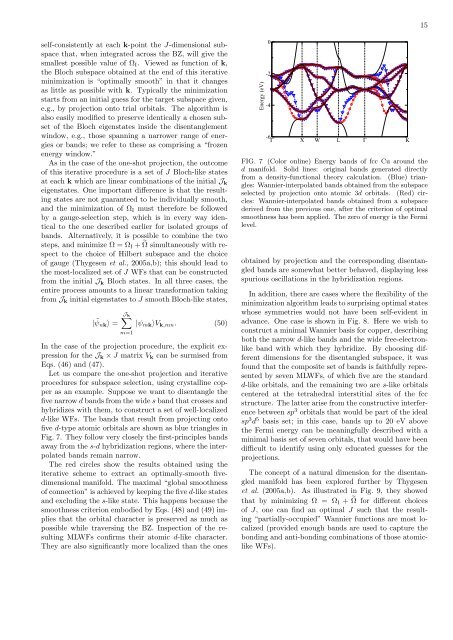The bands that result from projecting onto five d-type atomic orbitals are shown as blue triangles in Fig. 7. They follow very closely the first-principles bands away from the s-d hybridization regions, where the interpolated bands remain narrow. The red circles show the results obtained using the iterative scheme to extract an optimally-smooth fivedimensional manifold. The maximal “global smoothness of connection” is achieved by keeping the five d-like states and excluding the s-like state. This happens because the smoothness criterion embodied by Eqs. (48) and (49) implies that the orbital character is preserved as much as possible while traversing the BZ. Inspection of the resulting MLWFs confirms their atomic d-like character. They are also significantly more localized than the ones Energy (eV) 0 -2 -4 -6 Γ X W L Γ K FIG. 7 (Color online) Energy bands of fcc Cu around the d manifold. Solid lines: original bands generated directly from a density-functional theory calculation. (Blue) triangles: Wannier-interpolated bands obtained from the subspace selected by projection onto atomic 3d orbitals. (Red) circles: Wannier-interpolated bands obtained from a subspace derived from the previous one, after the criterion of optimal smoothness has been applied. The zero of energy is the Fermi level. obtained by projection and the corresponding disentangled bands are somewhat better behaved, displaying less spurious oscillations in the hybridization regions. In addition, there are cases where the flexibility of the minimization algorithm leads to surprising optimal states whose symmetries would not have been self-evident in advance. One case is shown in Fig. 8. Here we wish to construct a minimal Wannier basis for copper, describing both the narrow d-like bands and the wide free-electronlike band with which they hybridize. By choosing different dimensions for the disentangled subspace, it was found that the composite set of bands is faithfully represented by seven MLWFs, of which five are the standard d-like orbitals, and the remaining two are s-like orbitals centered at the tetrahedral interstitial sites of the fcc structure. The latter arise from the constructive interference between sp 3 orbitals that would be part of the ideal sp 3 d 5 basis set; in this case, bands up to 20 eV above the Fermi energy can be meaningfully described with a minimal basis set of seven orbitals, that would have been difficult to identify using only educated guesses for the projections. The concept of a natural dimension for the disentangled manifold has been explored further by Thygesen et al. (2005a,b). As illustrated in Fig. 9, they showed that by minimizing Ω = Ω I + ˜Ω for different choices of J, one can find an optimal J such that the resulting “partially-occupied” Wannier functions are most localized (provided enough bands are used to capture the bonding and anti-bonding combinations of those atomiclike WFs).
Page 1 and 2: Maximally localized Wannier functio
Page 3 and 4: 3 tition into separate “bands”,
Page 5 and 6: 5 such that ∇ k |u nk ⟩ is well
Page 7 and 8: 7 orbitals g n (r) corresponding to
Page 9 and 10: 9 to write down many alternative fi
Page 11 and 12: 11 To proceed further, we write dΩ
Page 13: 13 of the states in this larger man
Page 17 and 18: 17 Problems associated with reachin
Page 19 and 20: 19 FIG. 10 (Color online) Ethane (l
Page 21 and 22: 21 Energy (eV) -10 -15 Carbon s-orb
Page 23 and 24: 23 density operator in an LCAO basi
Page 25 and 26: 25 15 Energy (eV) 10 5 0 -5 Frozen
Page 27 and 28: 27 FIG. 19 (Color online) Contour-s
Page 29 and 30: 29 straightforward. The electric di
Page 31 and 32: 31 localization length near an insu
Page 33 and 34: 33 Giustino et al. (2003) and used
Page 35 and 36: 35 which is the desired k-space bul
Page 37 and 38: 37 FIG. 25 (Color online) Schematic
Page 39 and 40: 39 obtained by unfolding the Γ-poi
Page 41 and 42: 41 FIG. 31 (Color online) Surface d
Page 43 and 44: 43 One first evaluates certain obje
Page 45 and 46: 45 VII. WANNIER FUNCTIONS AS BASIS
Page 47 and 48: 47 the conductor to the leads (Datt
Page 49 and 50: 49 operators that are represented i
Page 51 and 52: 51 2. Self-interaction and DFT + Hu
Page 53 and 54: may be expressed as where c = (µ 0
Page 55 and 56: 55 1995; Bradley et al., 1995; Davi
Page 57 and 58: 57 Alfimov, G. L., P. G. Kevrekidis
Page 59 and 60: 59 Franchini, C., R. Kovacik, M. Ma
Page 61 and 62: 61 sity Press, Cambridge). Marzari,
Page 63 and 64: 63 Silvestrelli, P. L., and M. Parr

Maximally localized Wannier functions: Theory and applications

Create successful ePaper yourself

Delete template?

Save as template?