Maximally localized Wannier functions: Theory and applications

More documents

Recommendations

Info

20 Using |A ⊥ i ⟩ as a basis, the set of {ϕ n} which maximize L can be obtained using linear algebra as reported in Qian et al. (2008). Once a subspace with the correct orbital character has been identified, a basis of quasiatomic orbitals can be obtained by retaining the portion of the original AOs that “lives” on that subspace, |Q i ⟩ = J∑ |ϕ n ⟩⟨ϕ n |A i ⟩. (67) n=1 In general the angular dependence of the resulting QOs will no longer that of pure spherical harmonics, but only approximately so. In Qian et al. (2008), QOs were obtained for simple metals and semiconductors. Later applications have used the orbitals for the study of quantum transport in nano-structures (Qian et al., 2010). 2. NMTO and Downfolding An alternative scheme for obtaining a minimal basis representation is the perturbation approach introduced by Löwdin (1951). Here the general strategy is to partition a set of orbitals into an “active” set that is intended to describe the states of interest, and a “passive” set that will be integrated out. Let us write the Hamiltonian for the system in a block representation, H = ( ) H00 0 + 0 H 11 ( 0 V01 V 10 0 ) , (68) where H 00 (H 11 ) is the projection onto the active (passive) subspace, and V 01 is the coupling between the two subspaces. An eigenfunction can be written as the sum of its projections onto the two subspaces |ψ⟩ = |ψ 0 ⟩ + |ψ 1 ⟩. This leads to (H 00 − ε)|ψ 0 ⟩ + V 01 |ψ 1 ⟩ = 0, (69) V 10 |ψ 0 ⟩ + (H 11 − ε)|ψ 1 ⟩ = 0, (70) where ε is the eigenvalue corresponding to |ψ⟩. Elimination of |ψ 1 ⟩ gives an effective Hamiltonian for the system which acts only on the active subspace: H eff 00 (ε) = H 00 − V 01 (H 11 − ε) −1 V 10 . (71) This apparent simplification has introduced an energy dependence into the Hamiltonian. One practical way forward is to approximate this as an energy-independent Hamiltonian H00 eff (ε 0 ), choosing the reference energy ε 0 to be the average energy of the states of interest. This approach has been used to construct tight-binding Hamiltonians from full electronic structure calculations (Solovyev, 2004). A form of Löwdin partitioning has been widely used in connection with the linear-muffin-tin-orbital (LMTO) method, particularly in its most recent formulation, the N th -order muffin-tin-orbital (NMTO) approach (Andersen and Saha-Dasgupta, 2000; Zurek et al., 2005). In this context it is usually referred to as “downfolding”, although we note that some authors use this term to refer to any scheme to produce a minimal basis-set representation. In studies of complex materials there may be a significant number of MTOs, typically one for each angular momentum state (s, p, d) on every atomic site. One may wish to construct a minimal basis to describe states within a particular energy region, e.g., the occupied states, or those crossing the Fermi level. Let us assume we have of basis orbitals (MTOs in this case) which we wish to partition into “active” and “passive” sets. Using the notation of Eq. (68), Löwdin partitioning gives a set of energy-dependent orbitals ϕ 0 (ε, r) for the active space according to (Zurek et al., 2005) ϕ 0 (ε, r) = ϕ 0 (r) − ϕ 1 (r)(H 11 − ε) −1 V 10 . (72) Taking into account the energy dependence, this reduced set of orbitals spans the same space as the original full set of orbitals, and can be seen to be the original orbitals of the active set dressed by an energy-dependent linear combination of orbitals from the passive set. In the NMTO scheme, the next step is to form an energy-independent set of orbitals through an nth-order polynomial fit to the energy dependence. To give a specific example, accurate calculations on tetrahedral semiconductors will require the inclusion of d states in the MTO basis, i.e., nine states (s, p, d) per site. However, it would be desirable to construct a minimal basis to describe the valence and lower conduction states with only four states (s, p) on each site (Lambrecht and Andersen, 1986). We therefore designate s and p as “active” channels and d as “passive”. Downfolding will result in an MTO with either s or p character on a given site, with inclusion of d character on neighboring sites. In other words, the tail of the MTO is modified to “fold in” the character of the passive orbitals. In Fig. 11, the band structure of graphite calculated using a full s, p, and d basis on each carbon atom is shown in black (Zurek et al., 2005). The red bands are obtained by choosing s, p x , and p y states on every second carbon atom as the active channels and downfolding all other states. The energy mesh spans the energy range of the sp 2 bonding states (shown on the right-hand-side of the band-structure plot in Fig. 11). For these bands the agreement with the full calculation is perfect to within the resolution of the figure. Symmetric orthonormalization of the three NMTOs gives the familiar set of three symmetry related σ-bonding orbitals (compare with the MLWF of graphene in Fig. 6). Lechermann et al. (2006) have compared MLWFs and NMTO orbitals for a set of t 2g states located around the Fermi level SrVO 3 . It
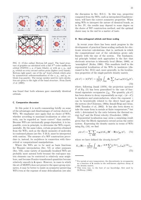
21 Energy (eV) -10 -15 Carbon s-orbital Carbon p x -orbital Carbon p y -orbital isosurface = +/- 0.04 isosurface = +/- 0.04 isosurface = +/- 0.04 15 10 5 0 -5 Γ Graphite σ bonding-bands K M Γ A L H A E 2 E 1 E 0 Carbon sp 2 -bond orbital isosurface = +/- 0.1 FIG. 11 (Color online) Bottom left panel: The band structure of graphite as calculated with a full N th -order muffin-tin orbital (NMTO) s, p, d basis (black), or with an s, p x, and p y orbital on every second carbon atom (lighter (red) bands). Bottom right panel: one of the sp 2 bond orbitals which arise by symmetrical orthonormalization of the s, p x, and p y orbitals (top panels). The energy meshes used for each calculation are given to the right of the band structure. From Zurek et al. (2005). was found that both schemes gave essentially identical orbitals. C. Comparative discussion At this point it is worth commenting briefly on some of the advantages and disadvantages of various choices of WFs. We emphasize once again that no choice of WFs, whether according to maximal localization or other criteria, can be regarded as “more correct” than another. Because WFs are intrinsically gauge-dependent, it is impossible, even in principle, to determine the WFs experimentally. By the same token, certain properties obtained from the WFs, such as the dipole moments of molecules in condensed phases (see Sec. V.B.3), must be interpreted with caution. The measure of a WF construction procedure is, instead, its usefulness in connection with theoretical or computational manipulations. Where the WFs are to be used as basis functions for Wannier interpolation (Sec. VI) or other purposes (Sec. VII), some variety of maximally localized WFs are probably most natural both because the real-space matrix elements can be restricted to relatively near neighbors, and because Fourier-transformed quantities become relatively smooth in k space. However, in cases in which the set of MLWFs does not preserve the space-group symmetry, it may be better to insist on symmetry-preserving WFs even at the expense of some delocalization (see also the discussion in Sec. II.I.1). In this way, properties computed from the WFs, such as interpolated bandstructures, will have the correct symmetry properties. When using WFs to interpret the nature of chemical bonds, as in Sec. IV, the results may depend to some degree on the choice of WF construction method, and the optimal choice may in the end be a matter of taste. D. Non-orthogonal orbitals and linear scaling In recent years there has been much progress in the development of practical linear-scaling methods for electronic structure calculations, that is, methods in which the computational cost of the calculation grows only linearly with the size of the system. The fundamental principle behind such approaches is the fact that electronic structure is inherently local (Heine, 1980), or ‘nearsighted’ (Kohn, 1996). This manifests itself in the exponential localization of the WFs in insulators (discussed in Sec. II.G) and, more generally, in the localization properties of the single-particle density matrix ρ(r, r ′ ) = ⟨r|P |r ′ ⟩ = V (2π) ∫BZ 3 dk ∑ f nk ψ nk (r)ψnk(r ∗ ′ ), n (73) where, following Janak (1978), the projection operator P of Eq. (5) has been generalized to the case of fractional eigenstate occupancies f nk . The quantity ρ(r, r ′ ) has been shown to decay exponentially as exp(−γ|r−r ′ |) in insulators and semiconductors, where the exponent γ can be heuristically related to the direct band gap of the system (des Cloizeaux, 1964a; Ismail-Beigi and Arias, 1999; Taraskin et al., 2002). It has also been shown to take the same form in metals at finite temperature, 9 but with γ determined by the ratio between the thermal energy k B T and the Fermi velocity (Goedecker, 1998). Exponential localization may seem a surprising result given that the Bloch eigenstates extend across the entire system. Expressing the density matrix in terms of WFs using Eq. (10), we find ρ(r, r ′ ) = ∑ ∑ w iR (r)K ij (R ′ − R)wjR ∗ ′(r′ ), (74) ij RR ′ where we have defined the density kernel 10 K ij (R) = V (2π) 3 ∫BZ dk e −ik·R ∑ n [U (k)† ] in f nk [U (k) ] nj , (75) 9 For metals at zero temperature, the discontinuity in occupancies as a function of k results in the well-known algebraic decay of the density matrix. 10 This term was, to the best of our knowledge, first used by McWeeny (1960).
Page 1 and 2: Maximally localized Wannier functio
Page 3 and 4: 3 tition into separate “bands”,
Page 5 and 6: 5 such that ∇ k |u nk ⟩ is well
Page 7 and 8: 7 orbitals g n (r) corresponding to
Page 9 and 10: 9 to write down many alternative fi
Page 11 and 12: 11 To proceed further, we write dΩ
Page 13 and 14: 13 of the states in this larger man
Page 15 and 16: 15 self-consistently at each k-poin
Page 17 and 18: 17 Problems associated with reachin
Page 19: 19 FIG. 10 (Color online) Ethane (l
Page 23 and 24: 23 density operator in an LCAO basi
Page 25 and 26: 25 15 Energy (eV) 10 5 0 -5 Frozen
Page 27 and 28: 27 FIG. 19 (Color online) Contour-s
Page 29 and 30: 29 straightforward. The electric di
Page 31 and 32: 31 localization length near an insu
Page 33 and 34: 33 Giustino et al. (2003) and used
Page 35 and 36: 35 which is the desired k-space bul
Page 37 and 38: 37 FIG. 25 (Color online) Schematic
Page 39 and 40: 39 obtained by unfolding the Γ-poi
Page 41 and 42: 41 FIG. 31 (Color online) Surface d
Page 43 and 44: 43 One first evaluates certain obje
Page 45 and 46: 45 VII. WANNIER FUNCTIONS AS BASIS
Page 47 and 48: 47 the conductor to the leads (Datt
Page 49 and 50: 49 operators that are represented i
Page 51 and 52: 51 2. Self-interaction and DFT + Hu
Page 53 and 54: may be expressed as where c = (µ 0
Page 55 and 56: 55 1995; Bradley et al., 1995; Davi
Page 57 and 58: 57 Alfimov, G. L., P. G. Kevrekidis
Page 59 and 60: 59 Franchini, C., R. Kovacik, M. Ma
Page 61 and 62: 61 sity Press, Cambridge). Marzari,
Page 63 and 64: 63 Silvestrelli, P. L., and M. Parr

Maximally localized Wannier functions: Theory and applications

Create successful ePaper yourself

Delete template?

Save as template?