Maximally localized Wannier functions: Theory and applications

43
One first evaluates certain objects in the Wannier gauge
using Bloch sums, and then transform to the Hamiltonian
gauge. Because the gauge transformation mixes the
bands, it is convenient to introduce a generalization of
Eq. (96) having two band indices instead of one. To this
end we start from Eq. (109) and define the matrices
Ω αβ = ∂ α A β − ∂ β A α = i⟨∂ α u|∂ β u⟩ − i⟨∂ β u|∂ α u⟩, (112)
where every object in this expression should consistently
carry either an H or W label. Provided that the chosen
WFs correctly span all occupied states, the integrand
of Eq. (110) can now be expressed as Ω tot
αβ
∑ =
J
n=1 f nΩ H αβ,nn .
A useful expression for Ω H αβ
can be obtained with the
help of the gauge-transformation law for the Bloch states,
|u H k ⟩ = |uW k ⟩U k [Eq. (100)]. Differentiating both sides
with respect to k α and then inserting into Eq. (112)
yields, after a few manipulations,
Ω H αβ = Ω αβ − [ D α , A β
]
+
[
Dβ , A α
]
− i [Dα , D β ] , (113)
where D α = U † ∂ α U, and A α , Ω αβ are related to the
connection and curvature matrices in the Wannier gauge
through the definition O k = U † k OW k U k. Using the banddiagonal
elements of Eq. (113) in the expression for Ω tot
αβ
eventually leads to
Ω tot
αβ =
J∑
f n Ω αβ,nn +
n
J∑
(f m − f n ) ( D α,nm A β,mn
mn
− D β,nm A α,mn + iD α,nm D β,mn
)
.
(114)
This is the desired expression, which in the Wannier interpolation
scheme takes the place of the sum-over-states
formula. In contrast to Eq. (111), note that the summations
over bands now run over the small set of Wannierprojected
bands. (Alternatively, it is possible to recast
Eq. (114) in a manifestly gauge-invariant form such that
the trace can be carried out directly in the Wannier
gauge; this formulation was used by Lopez et al. (2012)
to compute both the AHC and the orbital magnetization
of ferromagnets.)
The basic ingredients going into Eq. (114) are the Wannier
matrix elements of the Hamiltonian and of the position
operator. From a knowledge of ⟨0|H|R⟩ the energy
eigenvalues and occupation factors, as well as the matrices
U and D α , can be found using band-structure interpolation
(Sec. VI.A). The information about A W α and
Ω W αβ
is instead encoded in the matrix elements ⟨0|r|R⟩,
as can be seen by inverting Eq. (23),
A W α
= ∑ R
e ik·R ⟨0|r α |R⟩. (115)
As for Ω W αβ
, according to Eq. (112) it is given by the curl
of this expression, which can be taken analytically.
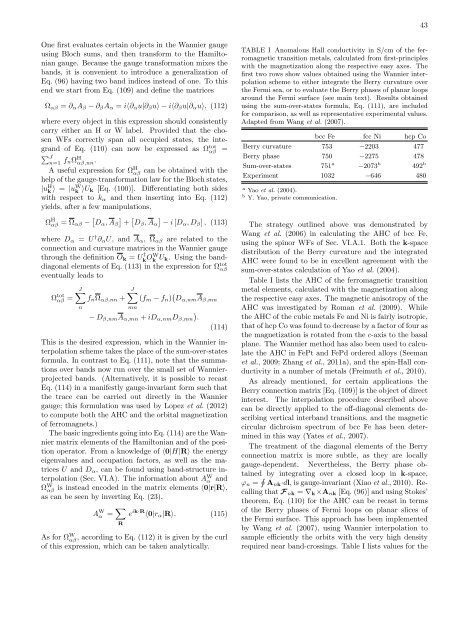
TABLE I Anomalous Hall conductivity in S/cm of the ferromagnetic
transition metals, calculated from first-principles
with the magnetization along the respective easy axes. The
first two rows show values obtained using the Wannier interpolation
scheme to either integrate the Berry curvature over
the Fermi sea, or to evaluate the Berry phases of planar loops
around the Fermi surface (see main text). Results obtained
using the sum-over-states formula, Eq. (111), are included
for comparison, as well as representative experimental values.
Adapted from Wang et al. (2007).
bcc Fe fcc Ni hcp Co
Berry curvature 753 −2203 477
Berry phase 750 −2275 478
Sum-over-states 751 a −2073 b 492 b
Experiment 1032 −646 480
a Yao et al. (2004).
b Y. Yao, private communication.
The strategy outlined above was demonstrated by
Wang et al. (2006) in calculating the AHC of bcc Fe,
using the spinor WFs of Sec. VI.A.1. Both the k-space
distribution of the Berry curvature and the integrated
AHC were found to be in excellent agreement with the
sum-over-states calculation of Yao et al. (2004).
Table I lists the AHC of the ferromagnetic transition
metal elements, calculated with the magnetization along
the respective easy axes. The magnetic anisotropy of the
AHC was investigated by Roman et al. (2009). While
the AHC of the cubic metals Fe and Ni is fairly isotropic,
that of hcp Co was found to decrease by a factor of four as
the magnetization is rotated from the c-axis to the basal
plane. The Wannier method has also been used to calculate
the AHC in FePt and FePd ordered alloys (Seeman
et al., 2009; Zhang et al., 2011a), and the spin-Hall conductivity
in a number of metals (Freimuth et al., 2010).
As already mentioned, for certain applications the
Berry connection matrix [Eq. (109)] is the object of direct
interest. The interpolation procedure described above
can be directly applied to the off-diagonal elements describing
vertical interband transitions, and the magnetic
circular dichroism spectrum of bcc Fe has been determined
in this way (Yates et al., 2007).
The treatment of the diagonal elements of the Berry
connection matrix is more subtle, as they are locally
gauge-dependent. Nevertheless, the Berry phase obtained
by integrating over a closed loop in k-space,
φ n = ∮ A nk·dl, is gauge-invariant (Xiao et al., 2010). Recalling
that F nk = ∇ k ×A nk [Eq. (96)] and using Stokes’
theorem, Eq. (110) for the AHC can be recast in terms
of the Berry phases of Fermi loops on planar slices of
the Fermi surface. This approach has been implemented
by Wang et al. (2007), using Wannier interpolation to
sample efficiently the orbits with the very high density
required near band-crossings. Table I lists values for the