Evaluation of the coefficient of subgrade reaction for ... - Marchetti DMT
Evaluation of the coefficient of subgrade reaction for ... - Marchetti DMT
Evaluation of the coefficient of subgrade reaction for ... - Marchetti DMT

Create successful ePaper yourself
Turn your PDF publications into a flip-book with our unique Google optimized e-Paper software.
<strong>Evaluation</strong> <strong>of</strong> <strong>the</strong> <strong>coefficient</strong> <strong>of</strong> <strong>subgrade</strong> <strong>reaction</strong> <strong>for</strong> design <strong>of</strong> multipropped<br />
diaphragm walls from <strong>DMT</strong> moduli<br />
P. Monaco & S. <strong>Marchetti</strong><br />
University <strong>of</strong> L'Aquila, Italy<br />
Keywords: Diaphragm walls, Subgrade Reaction Method, Flat Dilatometer Test<br />
ABSTRACT: This paper presents <strong>the</strong> preliminary results <strong>of</strong> a numerical study on multi-propped walls retaining deep<br />
excavations. The study is based on <strong>the</strong> comparison between <strong>the</strong> results obtained by FEM (Plaxis) using <strong>the</strong> non linear<br />
Hardening Soil model and by <strong>the</strong> Subgrade Reaction Method, considering different wall / soil stiffness, excavation depth<br />
and prop spacing conditions. A tentative relation, "calibrated" vs FEM results, is proposed <strong>for</strong> deriving <strong>the</strong> <strong>coefficient</strong><br />
<strong>of</strong> <strong>subgrade</strong> <strong>reaction</strong> K h <strong>for</strong> design <strong>of</strong> multi-propped diaphragm walls from <strong>the</strong> constrained modulus M from <strong>DMT</strong>.<br />
1 INTRODUCTION<br />
Multi-propped or multi-anchored diaphragm walls are<br />
widely used today <strong>for</strong> retaining deep open pit excavations<br />
in urban areas (e.g. underground car parkings), <strong>of</strong>ten in<br />
combination with <strong>the</strong> "top-down" construction technique,<br />
in order to limit <strong>the</strong> de<strong>for</strong>mations in <strong>the</strong> surrounding soil.<br />
The design <strong>of</strong> multi-restrained retaining walls requires<br />
<strong>the</strong> use <strong>of</strong> methods <strong>of</strong> analysis which take into account<br />
<strong>the</strong> soil-structure interaction and permit to simulate <strong>the</strong><br />
staged construction sequence. Though <strong>the</strong> Finite Element<br />
Method (FEM) approach is generally regarded today as<br />
<strong>the</strong> "way to <strong>the</strong> future", in common practice <strong>the</strong> simple<br />
and well-known Subgrade Reaction Method (SRM) or<br />
"spring method" is still widely used and <strong>of</strong>ten preferred to<br />
more sophisticated FEM analyses, particularly in <strong>the</strong><br />
early stage <strong>of</strong> design. The SRM permits to model even<br />
relatively complex cases in a simple and quick way, providing<br />
in general sufficiently reliable values <strong>of</strong> stresses in<br />
<strong>the</strong> wall and supports. On <strong>the</strong> o<strong>the</strong>r hand <strong>the</strong> SRM has<br />
several drawbacks, deriving from <strong>the</strong> rough simplification<br />
assumed in simulating <strong>the</strong> response <strong>of</strong> <strong>the</strong> soil to wall<br />
movements. One critical shortcoming is <strong>the</strong> difficulty in<br />
evaluating <strong>the</strong> <strong>coefficient</strong> <strong>of</strong> <strong>subgrade</strong> <strong>reaction</strong> K h on a rational<br />
base. K h is by no means an intrinsic property <strong>of</strong> <strong>the</strong><br />
soil. Its value depends not only on soil stiffness, but also<br />
on various "geometric-mechanical" factors (e.g. geometry<br />
and stiffness <strong>of</strong> wall / struts, excavation depth). Yet <strong>the</strong> influence<br />
<strong>of</strong> <strong>the</strong> above factors on K h is not clearly understood.<br />
Hence indications <strong>for</strong> <strong>the</strong> selection <strong>of</strong> K h values<br />
dependable <strong>for</strong> design may be helpful to many engineers<br />
who still rely on <strong>the</strong> "old" SRM <strong>for</strong> everyday practice.<br />
This paper presents <strong>the</strong> preliminary results <strong>of</strong> a numerical<br />
study aimed at establishing tentative correlations<br />
<strong>for</strong> deriving K h <strong>for</strong> design <strong>of</strong> multi-propped diaphragm<br />
walls from <strong>the</strong> constrained modulus M <strong>DMT</strong> obtained from<br />
<strong>the</strong> flat dilatometer test (<strong>Marchetti</strong> 1980). Comparisons<br />
both in terms <strong>of</strong> M <strong>DMT</strong> vs "reference" M and in terms <strong>of</strong><br />
predicted vs measured settlements (see reference list in<br />
TC16 2001) have shown that, in general, M <strong>DMT</strong> is a reasonably<br />
accurate "operative" modulus.<br />
The study is based on <strong>the</strong> comparison between FEM<br />
and SRM results, according to <strong>the</strong> following procedure:<br />
(1) Analysis <strong>of</strong> <strong>the</strong> behavior <strong>of</strong> a multi-propped wall <strong>for</strong><br />
various cases by FEM (Plaxis) using <strong>the</strong> non linear Hardening<br />
Soil model, with soil stiffness parameters estimated<br />
from M <strong>DMT</strong> . (2) Analysis by SRM varying K h until <strong>the</strong> results<br />
obtained by Plaxis <strong>for</strong> <strong>the</strong> same cases are appropriately<br />
reproduced. (3) Formulation <strong>of</strong> a tentative relation<br />
between backcalculated "best fit" K h values (matching<br />
FEM results) and M <strong>DMT</strong> .<br />
The study is purely numerical. K h values are "calibrated"<br />
based on FEM results, assumed herein to represent<br />
<strong>the</strong> "true" wall / soil behavior. No comparisons are<br />
shown between <strong>the</strong> behavior predicted by <strong>the</strong> models and<br />
observed in real cases.<br />
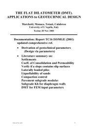
2 SPRING MODEL VS CONTINUUM<br />
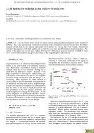
In <strong>the</strong> spring model <strong>the</strong> soil is schematized by a set <strong>of</strong> independent<br />
horizontal springs, generally characterized by a<br />
bilinear elastic-plastic pressure-displacement relation<br />
(Fig. 1). The <strong>coefficient</strong> <strong>of</strong> <strong>subgrade</strong> <strong>reaction</strong> K h (spring<br />
stiffness) is <strong>the</strong> initial slope <strong>of</strong> <strong>the</strong> curve until <strong>the</strong> limit<br />
pressure, active or passive, is reached. Hence a purely 2-<br />
D (plane strain) problem is converted into a 1-D problem.<br />
The soil behavior is "captured" by only one parameter,<br />
K h . The simplest case <strong>of</strong> homogeneous isotropic linear<br />
elastic continuum requires a minimum <strong>of</strong> two parameters<br />
(E and ν, or G and K) to fully define it.<br />
In general, it is not possible to establish a unique and<br />
straight<strong>for</strong>ward correlation between K h and soil stiffness<br />
E. Deriving K h <strong>of</strong> <strong>the</strong> springs from E <strong>of</strong> <strong>the</strong> continuum involves<br />
trying to establish a link between parameters <strong>of</strong><br />
different models. Yet engineers are familiar with moduli<br />
E, not with K h , and many times even crude relations E to<br />
K h may prove useful.<br />
Typical ranges <strong>of</strong> K h can be found in <strong>the</strong> literature, but<br />
great care is required owing to <strong>the</strong> problem-dependent nature<br />
<strong>of</strong> <strong>the</strong> parameter. For a given soil, values appropriate<br />
<strong>for</strong> strips, rafts, laterally loaded piles and flexible walls<br />
are all different (Clayton et al. 1993).<br />
3 EXISTING K h FORMULATIONS FOR WALLS<br />
Various methods have been proposed <strong>for</strong> evaluating K h<br />
<strong>for</strong> retaining walls (e.g. Terzaghi 1955, Ménard et al.<br />
1964, Balay 1984, Becci & Nova 1987, Schmitt 1995,<br />
Simon 1995). Most <strong>for</strong>mulations assume that K h [F⋅L -3 ] is<br />
directly proportional to <strong>the</strong> soil modulus E [F⋅L -2 ]. In essence,<br />
almost all studies arrive to similar conversion
Fig. 1. Typical pressure-displacement relation <strong>of</strong> <strong>the</strong> springs<br />
<strong>for</strong>mulae K h ∼ E / B, where B is a dimension [L] which<br />
represents <strong>the</strong> width <strong>of</strong> <strong>the</strong> soil area "loaded" by <strong>the</strong> wall.<br />
Most existing methods give indications <strong>for</strong> evaluating<br />
B <strong>for</strong> <strong>the</strong> simple mechanism <strong>of</strong> cantilever wall, generally<br />
suggesting to assume B proportional to <strong>the</strong> free cantilever<br />
height or embedded length. The behavior <strong>of</strong> multirestrained<br />
walls is more complex and <strong>the</strong> estimate <strong>of</strong> B is<br />
uncertain, since <strong>the</strong> earth pressure distribution and <strong>the</strong><br />
mode <strong>of</strong> de<strong>for</strong>mation <strong>of</strong> <strong>the</strong> wall are not known a priori.<br />
E.g. multi-propped thick concrete diaphragm walls constructed<br />
by top-down technique, with basement floor<br />
slabs used as struts, generally exhibit a very stiff "boxtype"<br />
behavior. The earth pressure may remain close to<br />
K 0 and multiple restraints permit only very small wall<br />
displacements. Hence K h (ratio pressure / displacement) is<br />
expected to be higher, i.e. B lower, than <strong>for</strong> cantilever<br />
walls. FEM studies on propped and cantilever walls by<br />
Potts & Fourie (1984, 1986) and Fourie & Potts (1989)<br />
pointed out <strong>the</strong> enormous importance <strong>of</strong> <strong>the</strong> mode <strong>of</strong> de<strong>for</strong>mation<br />
and displacement restraint on <strong>the</strong> earth pressure<br />
distribution and <strong>the</strong> resultant wall bending moments.<br />
Various contributions on K h given by French researchers<br />
are based on <strong>the</strong> original method by Ménard et al.<br />
(1964), which derives K h over <strong>the</strong> embedded length <strong>of</strong> a<br />
cantilever wall from <strong>the</strong> pressuremeter modulus E M :<br />
K h = E M / [α ⋅ a / 2 + 0.13 (9 a) α ] (1)<br />
This <strong>for</strong>mula contains a dimensional parameter a (in m)<br />
related to wall geometry and a non dimensional factor α<br />
related to soil type. Ménard et al. (1964) assumed a = 2/3<br />
<strong>of</strong> <strong>the</strong> embedded wall length (≈ distance between bottom<br />
<strong>of</strong> excavation and center <strong>of</strong> rotation at <strong>the</strong> toe <strong>of</strong> <strong>the</strong> wall).<br />
In practice a = height over which <strong>the</strong> soil is loaded by<br />
passive pressure. (Similar indications were given by Terzaghi<br />
1955).<br />
As reported by Amar et al. (1991), <strong>the</strong> pressuremeter<br />
modulus E M is related to <strong>the</strong> oedometer modulus (in <strong>the</strong><br />
same range <strong>of</strong> pressure) by <strong>the</strong> ratio E oed = E M / α. For NC<br />
soils α varies between 1/3 in sands to 2/3 in clays (Ménard<br />
& Rousseau 1962). In principle, M <strong>DMT</strong> (1-D modulus<br />
from <strong>DMT</strong>) can be used in Eq. 1 or derived <strong>for</strong>mulae in<br />
place <strong>of</strong> E M / α. (Various studies, e.g. Kalteziotis et al.<br />
1991, Ortigao et al. 1996, Brown & Vinson 1998, have<br />
quoted similar ratios - generally ≈ 1/2 - between PMT and<br />
<strong>DMT</strong> moduli in different soils).<br />
Balay (1984) adapted <strong>the</strong> Ménard <strong>for</strong>mulation <strong>for</strong><br />
evaluating K h over <strong>the</strong> entire wall length, assuming a = H<br />
(free cantilever height) above excavation level, while below<br />
<strong>the</strong> excavation a is related to <strong>the</strong> embedded length D<br />
and to <strong>the</strong> ratio D / H.<br />
Schmitt (1995), based on <strong>the</strong> observation <strong>of</strong> different<br />
modes <strong>of</strong> de<strong>for</strong>mation <strong>of</strong> stiff and flexible walls, adapted<br />
<strong>the</strong> Ménard <strong>for</strong>mulation to take into account <strong>the</strong> flexural<br />
inertia <strong>of</strong> <strong>the</strong> wall EI, assuming a ∼ (EI/ E oed ) 0.33 and<br />
E oed = E M / α, thus obtaining:<br />
K h = 2.1 (E 4/3 oed / EI 1/3 ) (2)<br />
According to <strong>the</strong> above relation, <strong>for</strong> a given soil modulus<br />
a stiff wall would have a lower K h than a flexible wall.<br />
(Earlier studies on spread footings had indicated a lower<br />
influence <strong>of</strong> structure stiffness on K, e.g. Vesic 1961<br />
found K inversely proportional to EI 1/12 ).<br />
Simon (1995) extended <strong>the</strong> Ménard <strong>for</strong>mulation<br />
adapted by Balay (1984) differentiating K h <strong>for</strong> zones <strong>of</strong><br />
"free" de<strong>for</strong>mations (free height and embedded length <strong>of</strong><br />
cantilever wall) and "restrained" de<strong>for</strong>mations (zones between<br />
two props / anchors and behind a pretensioned anchor).<br />
For <strong>the</strong> zone between two props at distance L, assuming<br />
that a foundation <strong>of</strong> width B causes de<strong>for</strong>mations<br />
over a length L ≈ 1.5 B, Simon (1995) proposed:<br />
K h = E M / [0.13 (4.4 B) α + α ⋅ B / 6] (3)<br />
The method by Becci & Nova (1987) differs from o<strong>the</strong>r<br />
spring methods <strong>for</strong> taking into account <strong>the</strong> non linear soil<br />
behavior, assuming <strong>the</strong> soil modulus E varying with stress<br />
level and loading path direction. K h is evaluated as:<br />
K h = a ⋅ E / L (4)<br />
E is assumed as <strong>the</strong> unloading-reloading modulus E ur<br />
where <strong>the</strong> present stress level is lower than <strong>the</strong> maximum<br />
past stress level, as <strong>the</strong> virgin compression modulus when<br />
<strong>the</strong> maximum past stresses are exceeded. a is a non dimensional<br />
empirical factor (<strong>the</strong> Authors assume a = 1).<br />
As first approximation, L (≈ width <strong>of</strong> soil zone involved<br />
by <strong>the</strong> wall movement) is assumed as an "average" width<br />
<strong>of</strong> <strong>the</strong> Rankine active and passive pressure wedges behind<br />
and in front <strong>of</strong> <strong>the</strong> wall (this leads to different K h on <strong>the</strong><br />
two sides).<br />
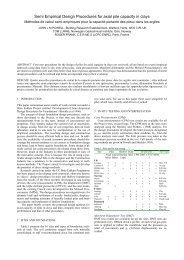
4 FEM INPUT PARAMETERS<br />
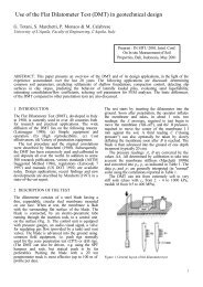
The geometry <strong>of</strong> <strong>the</strong> multi-propped wall selected <strong>for</strong> this<br />
study (Fig. 2) reproduces a typical configuration <strong>of</strong> common<br />
excavation works (e.g. car parking with 6 basement<br />
floors). The final depth <strong>of</strong> <strong>the</strong> excavation is 18 m. The total<br />
length <strong>of</strong> <strong>the</strong> wall is 24 m (embedded length 6 m). Six<br />
prop levels are equally spaced at 3 m intervals. The upper<br />
prop level is placed just at <strong>the</strong> top <strong>of</strong> <strong>the</strong> wall (ground surface).<br />
The half-width <strong>of</strong> <strong>the</strong> excavation is 20 m.<br />
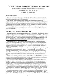
The finite element mesh used in Plaxis (plane strain<br />
analysis) is shown in Fig. 3. The wall was schematized as<br />
a "beam" element. The props were simulated by Plaxis<br />
"fixed-end anchor" elements (elastic springs <strong>of</strong> given axial<br />
stiffness, having one "movable" end connected to <strong>the</strong><br />
wall and <strong>the</strong> o<strong>the</strong>r end "fixed" - zero displacement - at<br />
given longitudinal distance from <strong>the</strong> wall).<br />
The soil behavior was simulated using <strong>the</strong> non linear<br />
Hardening Soil (HS) model <strong>of</strong> <strong>the</strong> Plaxis code. This<br />
model requires to input three stiffness moduli at <strong>the</strong> reference<br />
pressure p ref = 100 kPa: <strong>the</strong> tangent oedometer<br />
modulus E ref oed , <strong>the</strong> triaxial modulus E ref 50 , <strong>the</strong> unloadingreloading<br />
modulus E ref ur . All moduli are stress-level dependent,<br />
according to <strong>the</strong> expressions E oed = E oed<br />
ref<br />
(σ' 1 / p ref ) m ref<br />
, E 50 = E 50 (σ' 3 / p ref ) m ref<br />
, E ur = E ur (σ' 3 / p ref ) m ,<br />
where σ' 1 and σ' 3 are <strong>the</strong> major and minor principal effective<br />
stresses. (Usually m ≈ 0.5 to 1).<br />
An intensive literature survey by Schanz & Vermeer<br />
(1997) indicated <strong>for</strong> remolded quartz sands (from very<br />
loose silty sands to very dense gravelly sands) E ref 50 = 15<br />
to 75 MPa. The above range is remarkably similar to <strong>the</strong><br />
range <strong>of</strong> M <strong>DMT</strong> values found <strong>for</strong> sands <strong>of</strong> similar density.<br />
Schanz & Vermeer (1997) showed that E ref 50 is correlated<br />
to <strong>the</strong> 1-D modulus E ref oed . Hence, if one has data on <strong>the</strong><br />
oedometer modulus, it can be used to estimate <strong>the</strong> triaxial
Fig. 2. Geometry <strong>of</strong> multi-propped wall<br />
100 m<br />
100 m 20 m<br />
wall<br />
excavation<br />
Fig. 3. Finite element mesh <strong>for</strong> multi-propped wall study<br />
modulus. Based on <strong>the</strong> above considerations, in this study<br />
it was assumed E oed = M <strong>DMT</strong> , and all moduli required by<br />
<strong>the</strong> Plaxis HS model were estimated assuming M <strong>DMT</strong> as<br />
<strong>the</strong> basic reference stiffness parameter. According to indications<br />
given by Plaxis researchers (Vermeer 2001), <strong>the</strong><br />
following "typical" ratios between different moduli were<br />
ref<br />
adopted: E 50 = E ref ref<br />
oed , E ur = 4 E ref oed .<br />
Two soil types were considered: a "s<strong>of</strong>t soil" (e.g. a<br />
s<strong>of</strong>t to medium clay) having M <strong>DMT</strong> = 4 MPa and a "stiff<br />
soil" (e.g. a hard clay or a medium dense sand) having<br />
M <strong>DMT</strong> = 40 MPa (at p ref = 100 kPa). The above M <strong>DMT</strong> values<br />
were selected to generally characterize a wide category<br />
<strong>of</strong> s<strong>of</strong>t and stiff soils, and do not refer to any particular<br />
site. Having a real M <strong>DMT</strong> pr<strong>of</strong>ile from a specific site <strong>for</strong><br />
ref<br />
a homogeneous soil, one could assume E oed = M <strong>DMT</strong> at<br />
σ' v = 100 kPa. Also, <strong>the</strong> exponent m could be inferred<br />
from <strong>the</strong> rate <strong>of</strong> increase <strong>of</strong> M <strong>DMT</strong> with depth.<br />
The only difference between <strong>the</strong> "s<strong>of</strong>t soil" and <strong>the</strong><br />
"stiff soil" relates to stiffness. The "stiff soil" is simply a<br />
factor 10 stiffer than <strong>the</strong> "s<strong>of</strong>t soil", but <strong>the</strong> relation E 50 /<br />
E oed / E ur is 1/1/4 <strong>for</strong> both soils. For both soils it was assumed<br />
m = 0.5 and ν ur = 0.2 (Poisson's ratio <strong>for</strong> unloading-reloading).<br />
All o<strong>the</strong>r parameters, in particular shear<br />
strength, were conveniently assumed equal <strong>for</strong> both soils:<br />
bulk unit weight γ = 19 kN/m 3 , friction angle Φ' = 30°, dilatancy<br />
angle ψ = 0, cohesion c' = 0.5 kPa, wall / soil friction<br />
angle δ = 20°. The wall was assumed to be installed<br />
without altering <strong>the</strong> in situ conditions ("wished in place").<br />
The initial stresses were calculated assuming K 0 = 0.5.<br />
The present study is restricted to fully drained conditions,<br />
with zero pore pressures everywhere. Seepage pressures<br />
have been ignored at this stage <strong>of</strong> <strong>the</strong> study, in an<br />
attempt to investigate <strong>the</strong> effects <strong>of</strong> earth pressures alone<br />
on <strong>the</strong> wall behavior.<br />
Four different soil / wall stiffness combinations were<br />
considered (Table 1). The "rigid wall" is a 1 m thick rein<strong>for</strong>ced<br />
concrete diaphragm wall, having Young's modulus<br />
E = 25000 MPa. The "flexible wall" is a steel sheetpile<br />
wall <strong>of</strong> similar structural capacity. Note that Case A and<br />
Case D have similar wall / soil stiffness ratios (EI / E oed ref =<br />
58 and 52 respectively). For Case B EI / E oed ref = 521. For<br />
Case C EI / E oed ref = 5.8. Hence <strong>the</strong> wall / soil stiffness relation<br />
between <strong>the</strong> various cases is ≈ 1/10/100.<br />
Very stiff props (30 cm thick concrete slabs, axial<br />
stiffness EA = 7500 MN/m) are associated to <strong>the</strong> "rigid<br />
wall" scheme. The "flexible wall" is supported by steel<br />
props <strong>of</strong> lower stiffness (EA = 657 MN/m). No prestress<br />
<strong>for</strong>ce was given to <strong>the</strong> props. The excavation sequence<br />
was simulated assuming that each prop level, starting<br />
from <strong>the</strong> uppermost one, is installed be<strong>for</strong>e excavating <strong>the</strong><br />
3 m soil layer immediately below, down to <strong>the</strong> next prop<br />
level (as in <strong>the</strong> top-down technique).<br />
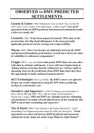
5 FEM RESULTS FOR MULTI-PROPPED WALL<br />
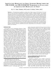
The results <strong>of</strong> Plaxis analyses obtained <strong>for</strong> Cases A, B, C<br />
and D at <strong>the</strong> maximum excavation depth (18 m) are<br />
summarized in Fig. 4. Observations:<br />
(a) The horizontal effective stresses developed on <strong>the</strong><br />
back and on <strong>the</strong> front <strong>of</strong> <strong>the</strong> wall resulting from Plaxis<br />
calculation are shown in Fig. 4, compared to <strong>the</strong> distributions<br />
<strong>of</strong> at-rest, active and passive earth pressures (K a and<br />
K p calculated according to Caquot & Kerisel 1948). In<br />
general <strong>the</strong> full active condition behind <strong>the</strong> wall is not<br />
reached and σ' h is intermediate between <strong>the</strong> initial K 0 and<br />
<strong>the</strong> K a line. The passive pressure K p is mobilized over ≈<br />
1/3 <strong>of</strong> <strong>the</strong> embedded wall length. Note that <strong>the</strong> earth pressure<br />
distribution is quite similar <strong>for</strong> Cases A and D, having<br />
similar wall / soil stiffness ratios.<br />
(b) An "anomalous" earth pressure distribution results<br />
from <strong>the</strong> combination stiff soil / flexible wall (Case C).<br />
The progressive deflections <strong>of</strong> <strong>the</strong> wall towards <strong>the</strong> excavation<br />
promote <strong>the</strong> redistribution <strong>of</strong> σ' h behind <strong>the</strong> wall in<br />
<strong>the</strong> embedded length and upper restrained zones (arching),<br />
while just above excavation level σ' h decreases even<br />
below <strong>the</strong> "<strong>the</strong>oretical" minimum K a . The maximum<br />
bending moment is much smaller than in all o<strong>the</strong>r cases,<br />
less than 50 % <strong>of</strong> <strong>the</strong> value calculated <strong>for</strong> <strong>the</strong> same soil in<br />
combination with <strong>the</strong> "rigid wall". A significant "fixity"<br />
moment at <strong>the</strong> toe <strong>of</strong> <strong>the</strong> wall is also observed in this case.<br />
(Similar results were obtained by Vermeer 2001 <strong>for</strong> a single-anchored<br />
wall <strong>of</strong> similar EI / E oed ratio).<br />
(c) The maximum horizontal displacements occur at ≈<br />
15-18 m depth, near <strong>the</strong> bottom <strong>of</strong> <strong>the</strong> excavation. The<br />
top <strong>of</strong> <strong>the</strong> wall does not move at all, due to <strong>the</strong> restraint<br />
provided by <strong>the</strong> upper props. This "deep" mode <strong>of</strong> de<strong>for</strong>mation<br />
is opposite to <strong>the</strong> cantilever-type.<br />
(d) The diagrams on <strong>the</strong> right in Fig. 4, inferred from<br />
Plaxis results, represent <strong>the</strong> variation <strong>of</strong> <strong>the</strong> earth pressure<br />
Table 1. Soil and wall stiffness parameters<br />
Soil stiffness E oed<br />
ref<br />
Case A<br />
s<strong>of</strong>t soil / flexible wall<br />
Case B<br />
s<strong>of</strong>t soil / rigid wall<br />
Case C<br />
stiff soil / flexible wall<br />
Case D<br />
stiff soil / rigid wall<br />
(MPa)<br />
Wall stiffness EI<br />
(MNm 2 /m)<br />
4 232<br />
4 2083<br />
40 232<br />
40 2083
Depth z (m)<br />
Depth z (m)<br />
Depth z (m)<br />
Depth z (m)<br />
0<br />
3<br />
6<br />
9<br />
12<br />
15<br />
18<br />
21<br />
K0 Ka<br />
Kp<br />
24<br />
-400 -200 0 200 400 600<br />
0<br />
3<br />
6<br />
9<br />
12<br />
15<br />
18<br />
Earth pressure σ'h (kPa)<br />
21<br />
K0 Ka<br />
Kp<br />
24<br />
-400 -200 0 200 400 600<br />
0<br />
3<br />
6<br />
9<br />
12<br />
15<br />
18<br />
Earth pressure σ'h (kPa)<br />
21<br />
K0 Ka<br />
Kp<br />
24<br />
-400 -200 0 200 400 600<br />
0<br />
3<br />
6<br />
9<br />
12<br />
15<br />
18<br />
FEM<br />
FEM<br />
Earth pressure σ'h (kPa)<br />
FEM<br />
Earth pressure σ'h (kPa)<br />
FEM<br />
21<br />
K0 Ka<br />
Kp<br />
24<br />
-400 -200 0 200 400 600<br />
z (m)<br />
z (m)<br />
z (m)<br />
z (m)<br />
0<br />
3<br />
6<br />
9<br />
12<br />
15<br />
18<br />
21<br />
24<br />
0 1 2 3 4 5 6 7<br />
0<br />
3<br />
6<br />
9<br />
12<br />
15<br />
18<br />
21<br />
Displacement y (cm)<br />
24<br />
0 1 2 3 4 5 6 7<br />
0<br />
3<br />
6<br />
9<br />
12<br />
15<br />
18<br />
21<br />
24<br />
0 1 2 3 4 5 6 7<br />
0<br />
3<br />
6<br />
9<br />
12<br />
15<br />
18<br />
21<br />
Displacement y (cm)<br />
FEM<br />
SRM best fit<br />
Kh = 800 kN/m 3<br />
B = 7.5 m<br />
FEM<br />
SRM best fit<br />
Kh = 2000 kN/m 3<br />
B = 3 m<br />
Displacement y (cm)<br />
FEM<br />
SRM best fit<br />
Kh = 10000 kN/m 3<br />
B = 6 m<br />
Displacement y (cm)<br />
FEM<br />
SRM best fit<br />
Kh = 8000 kN/m 3<br />
B = 7.5 m<br />
24<br />
0 1 2 3 4 5 6 7<br />
z (m)<br />
z (m)<br />
z (m)<br />
z (m)<br />
Bending moment M (kNm)<br />
0<br />
FEM<br />
3<br />
SRM best fit<br />
Kh = 800 kN/m 3<br />
6<br />
B = 7.5 m<br />
9<br />
12<br />
15<br />
18<br />
21<br />
24<br />
-250 0 250 500 750<br />
Bending moment M (kNm)<br />
0<br />
FEM<br />
3<br />
SRM best fit<br />
Kh = 2000 kN/m 3<br />
6<br />
B = 3 m<br />
9<br />
12<br />
15<br />
18<br />
21<br />
24<br />
-250 0 250 500 750<br />
Bending moment M (kNm)<br />
0<br />
FEM<br />
3<br />
SRM best fit<br />
Kh = 10000 kN/m 3<br />
6<br />
B = 6 m<br />
9<br />
12<br />
15<br />
18<br />
21<br />
24<br />
-250 0 250 500 750<br />
0<br />
3<br />
6<br />
9<br />
12<br />
15<br />
18<br />
21<br />
Bending moment M (kNm)<br />
FEM<br />
SRM best fit<br />
Kh = 8000 kN/m 3<br />
B = 7.5 m<br />
24<br />
-250 0 250 500 750<br />
CASE A<br />
SOFT SOIL / FLEXIBLE WALL<br />
K0<br />
Ka<br />
z = 16.5 m<br />
ACTIVE SIDE<br />
0.6 0.5 0.4 0.3<br />
0.6<br />
0.5<br />
0.4<br />
0.3<br />
z = 1.5 m<br />
0.2<br />
FEM<br />
0.1<br />
0.0<br />
0.2 0.1 0.0<br />
Normalized wall displacement y/z (%)<br />
CASE B<br />
SOFT SOIL / RIGID WALL<br />
0.6<br />
K0<br />
0.5<br />
0.4<br />
0.3<br />
Ka<br />
z = 16.5 m<br />
z = 1.5 m<br />
0.2<br />
0.1<br />
ACTIVE SIDE<br />
FEM<br />
0.0<br />
0.10 0.08 0.06 0.04 0.02 0.00<br />
Normalized wall displacement y/z (%)<br />
CASE C<br />
STIFF SOIL / FLEXIBLE WALL<br />
z = 1.5 m<br />
K0<br />
Ka<br />
ACTIVE SIDE<br />
0.6 0.5 0.4<br />
1.4<br />
1.2<br />
1.0<br />
0.8<br />
0.6<br />
0.4<br />
z = 16.5 m FEM<br />
0.2<br />
0.0<br />
0.3 0.2 0.1 0.0<br />
Normalized wall displacement y/z (%)<br />
CASE D<br />
STIFF SOIL / RIGID WALL<br />
0.6<br />
K0<br />
0.5<br />
0.4<br />
0.3<br />
Ka<br />
z = 16.5 m z = 1.5 m<br />
0.2<br />
0.1<br />
ACTIVE SIDE<br />
FEM<br />
0.0<br />
0.05 0.04 0.03 0.02 0.01 0.00<br />
Normalized wall displacement y/z (%)<br />
σ'h /σ'v on back <strong>of</strong> wall<br />
σ'h /σ'v on back <strong>of</strong> wall<br />
σ'h /σ'v on back <strong>of</strong> wall<br />
σ'h /σ'v on back <strong>of</strong> wall<br />
Fig. 4. Results <strong>of</strong> FEM and SRM analyses <strong>for</strong> multi-propped wall. Earth pressure distribution, horizontal wall displacements and<br />
bending moments at 18 m excavation depth. Normalized pressure–displacement curves on back <strong>of</strong> wall at 1.5 m depth intervals.
σ' h on <strong>the</strong> back <strong>of</strong> <strong>the</strong> wall vs <strong>the</strong> horizontal wall displacement<br />
y at various depths (each curve refers to a<br />
given depth z, at 1.5 m intervals). To compare curves obtained<br />
at different depths, σ' h is normalized to <strong>the</strong> vertical<br />
stress (earth pressure <strong>coefficient</strong> K = σ' h / σ' v ) and <strong>the</strong> horizontal<br />
displacement y is normalized to depth z (ratio y / z).<br />
The dashed horizontal lines represent <strong>the</strong> at-rest (initial)<br />
K 0 and <strong>the</strong> active K a pressure <strong>coefficient</strong>s. These curves<br />
correspond to <strong>the</strong> "active side" <strong>of</strong> <strong>the</strong> spring pressuredisplacement<br />
curve in Fig. 1. (The attention is focused<br />
here on <strong>the</strong> "active side", more significant than <strong>the</strong> "passive<br />
side" <strong>for</strong> multi-propped walls, since <strong>the</strong>ir embedded<br />
length is generally small compared to <strong>the</strong> retained height).<br />
The figures show that, as <strong>the</strong> wall moves towards <strong>the</strong> excavation,<br />
σ' h behind <strong>the</strong> wall varies differently from one<br />
case to ano<strong>the</strong>r. In general K a is not reached, except <strong>for</strong><br />
Case C. In Cases A, C and D, after an initial decrease, σ' h<br />
tends even to increase (well beyond K 0 in Case C) with<br />
wall displacement. (Again, <strong>the</strong> curves obtained <strong>for</strong> Cases<br />
A and D are quite similar). Only in Case B σ' h decreases<br />
continuously. In general, however, <strong>the</strong> slope <strong>of</strong> <strong>the</strong> "normalized"<br />
curves obtained at various depths <strong>for</strong> each case<br />
is similar. Since <strong>the</strong> slope <strong>of</strong> <strong>the</strong>se curves is equal to K h <strong>of</strong><br />
<strong>the</strong> springs (K h = ∆σ' h / ∆y) divided by <strong>the</strong> unit weight γ<br />
(assumed constant), this suggests that adopting K h constant<br />
with depth in spring calculations should not involve<br />
a large error, at least as first approximation.<br />
6 SPRING ANALYSIS RESULTS<br />
The Subgrade Reaction Method was used to simulate <strong>the</strong><br />
behavior <strong>of</strong> <strong>the</strong> multi-propped wall in Fig. 2, considering<br />
<strong>the</strong> same four cases analyzed by FEM. For each case<br />
SRM calculations were repeated varying K h until <strong>the</strong><br />
bending moments and <strong>the</strong> horizontal displacements <strong>of</strong> <strong>the</strong><br />
wall were nearly equal to <strong>the</strong> values calculated by Plaxis.<br />
As first approximation, K h were assumed constant<br />
with depth and through all calculation steps, and equal on<br />
both sides <strong>of</strong> <strong>the</strong> wall. (A better estimate would involve<br />
K h varying with depth and calculation sequence, e.g. K h<br />
decreasing as excavation depth increases, and possibly<br />
different on <strong>the</strong> active and passive side).<br />
The pr<strong>of</strong>iles <strong>of</strong> <strong>the</strong> horizontal displacements and bending<br />
moments calculated by SRM <strong>for</strong> <strong>the</strong> "best fit" K h , i.e.<br />
<strong>the</strong> K h values <strong>for</strong> which SRM results "match" FEM results<br />
(assuming <strong>the</strong> bending moment as "target" parameter), are<br />
shown in Fig. 4, superimposed to <strong>the</strong> Plaxis results. (The<br />
"best fit" K h <strong>for</strong> matching horizontal displacements may<br />
differ slightly). Observations:<br />
(a) The SRM reproduces well Plaxis results in Cases A<br />
and D, <strong>of</strong> "intermediate" wall / soil stiffness. The ratio between<br />
<strong>the</strong> "best fit" K h calculated <strong>for</strong> <strong>the</strong> above two cases<br />
(K h = 800 and 8000 kN/m 3 respectively) is equal to <strong>the</strong> ratio<br />
between <strong>the</strong> corresponding s<strong>of</strong>t / stiff soil moduli<br />
(1/10), confirming K h proportional to soil stiffness.<br />
(b) For Cases B and C, <strong>of</strong> "high" and "low" wall / soil<br />
stiffness respectively, <strong>the</strong> SRM is not able to reproduce<br />
Plaxis results with <strong>the</strong> same accuracy, even adopting different<br />
distributions <strong>of</strong> K h with depth. This result is presumably<br />
a consequence <strong>of</strong> <strong>the</strong> limited ability <strong>of</strong> <strong>the</strong> spring<br />
model to simulate <strong>the</strong> soil behavior in particular conditions<br />
(e.g. in Case C arching cannot be simulated, since<br />
<strong>the</strong> spring would yield plastically as soon as K a is reached<br />
and <strong>the</strong> earth pressure will never reach smaller values).<br />
The "best fit" backcalculated values are K h = 2000 kN/m 3<br />
<strong>for</strong> Case B, K h = 10000 kN/m 3 <strong>for</strong> Case C.<br />
The axial <strong>for</strong>ces in <strong>the</strong> props calculated <strong>for</strong> <strong>the</strong> "best fit"<br />
K h are generally in good agreement (± 10-20 %) with <strong>the</strong><br />
values calculated by Plaxis. Only in Case C <strong>the</strong> SRM<br />
largely underestimates (− 40-60 %) <strong>the</strong> <strong>for</strong>ces in <strong>the</strong> upper<br />
prop levels.<br />
The "best fit" K h backcalculated from Plaxis results<br />
were compared to <strong>the</strong> values determined by various existing<br />
K h <strong>for</strong>mulations. The range <strong>of</strong> K h obtained according<br />
to Eq. 4 by Becci & Nova (1987), assuming E = virgin<br />
compression modulus (not varying with stress, as first approximation),<br />
is similar to <strong>the</strong> "best fit" K h . Also <strong>the</strong> K h<br />
obtained according to Balay (1984) are not so far from<br />
<strong>the</strong> "best fit" K h . The <strong>for</strong>mulation by Schmitt (1995) overestimates<br />
K h , giving K h <strong>for</strong> <strong>the</strong> "rigid wall" less than 50 %<br />
<strong>of</strong> K h <strong>for</strong> <strong>the</strong> "flexible wall", in contrast with <strong>the</strong> results <strong>of</strong><br />
SRM-FEM comparison. The K h obtained according to <strong>the</strong><br />
<strong>for</strong>mula by Simon (1995) <strong>for</strong> <strong>the</strong> inter-prop zone are also<br />
overestimated.<br />
Hence, <strong>for</strong> <strong>the</strong> examined cases, existing K h <strong>for</strong>mulations<br />
taking into account wall / soil stiffness and restraint<br />
conditions do not reproduce <strong>the</strong> FEM-calculated behavior<br />
better than methods which do not take into account <strong>the</strong><br />
above factors.<br />
7 INFLUENCE OF EXCAVATION DEPTH AND<br />
PROP SPACING ON K h<br />
In order to investigate <strong>the</strong> influence <strong>of</strong> <strong>the</strong> excavation<br />
depth on K h , FEM and SRM calculations <strong>for</strong> <strong>the</strong> multipropped<br />
wall were repeated considering two different excavation<br />
depths, H = 12 m and H = 24 m. In both cases<br />
<strong>the</strong> embedded wall length was assumed equal to 6 m, as<br />
in <strong>the</strong> 18 m excavation previously considered.<br />
For each excavation depth (H = 12, 18 and 24 m) <strong>the</strong><br />
calculation was repeated assuming two different values <strong>of</strong><br />
prop spacing, s = 3 m and s = 6 m.<br />
This analysis was carried out only <strong>for</strong> <strong>the</strong> "rigid wall"<br />
(1 m thick concrete diaphragm wall).<br />
Besides <strong>the</strong> "s<strong>of</strong>t" and <strong>the</strong> "stiff" soil (E oed ref = 4 and 40<br />
MPa respectively), a soil <strong>of</strong> "intermediate" stiffness<br />
(E oed ref = 16 MPa) was also considered. The above values<br />
<strong>of</strong> E oed ref , relative to a reference pressure p ref = 100 kPa,<br />
correspond to average values <strong>of</strong> <strong>the</strong> constrained modulus<br />
M <strong>DMT</strong> over <strong>the</strong> entire wall length equal to M <strong>DMT</strong> ≈ 5-7 MPa<br />
<strong>for</strong> <strong>the</strong> "s<strong>of</strong>t" soil, M <strong>DMT</strong> ≈ 20-30 MPa <strong>for</strong> <strong>the</strong> "intermediate"<br />
soil and M <strong>DMT</strong> ≈ 50-70 MPa <strong>for</strong> <strong>the</strong> "stiff" soil.<br />
The "best fit" K h resulting from SRM-FEM comparison<br />
<strong>for</strong> <strong>the</strong> examined cases are shown in Figs. 5 and 6.<br />
Fig. 5 shows that, <strong>for</strong> given soil stiffness M <strong>DMT</strong> (average<br />
over total wall length) and prop spacing, K h decreases<br />
significantly as <strong>the</strong> excavation depth increases from 12 to<br />
18 m, but remains practically unchanged from 18 to 24 m.<br />
For given M <strong>DMT</strong> and excavation depth, K h decreases as<br />
prop spacing increases from 3 to 6 m, but such reduction<br />
is more pronounced <strong>for</strong> <strong>the</strong> lower depth (H = 12 m). In<br />
essence, K h decreases as excavation depth and prop spacing<br />
increase, but <strong>the</strong> influence <strong>of</strong> both factors on K h is<br />
smaller at higher excavation depths.<br />
Fig. 6 shows <strong>the</strong> variation <strong>of</strong> K h with M <strong>DMT</strong> (average<br />
over total wall length) <strong>for</strong> different values <strong>of</strong> excavation<br />
depth and prop spacing. K h increases with M <strong>DMT</strong> , as expected.<br />
In most cases, <strong>for</strong> a given value <strong>of</strong> M <strong>DMT</strong> , <strong>the</strong> values<br />
<strong>of</strong> K h vary over a relative narrow range. Only in <strong>the</strong><br />
case H = 12 m and s = 3 m (a nearly "zero displacement"<br />
restraint condition) K h is significantly higher.
Kh (kN/m 3 )<br />
Excavation depth H (m)<br />
Fig. 5. "Best fit" K h vs excavation depth H <strong>for</strong> different values<br />
<strong>of</strong> constrained soil modulus M <strong>DMT</strong> and prop spacing s<br />
Kh (kN/m 3 )<br />
20000<br />
15000<br />
10000<br />
5000<br />
20000<br />
15000<br />
10000<br />
1 m thick concrete<br />
diaphragm wall<br />
M<strong>DMT</strong> = 5-7 MPa<br />
M<strong>DMT</strong> = 20-30 MPa<br />
M<strong>DMT</strong> = 50-70 MPa<br />
s = 3 m<br />
s = 6 m<br />
0<br />
0 6 12 18 24 30<br />
1 m thick concrete<br />
diaphragm wall<br />
H = 12 m<br />
H = 18 m<br />
H = 24 m<br />
s = 3 m<br />
s = 6 m<br />
5-7 MPa, 0.2-0.4 <strong>for</strong> M <strong>DMT</strong> = 20-30 MPa and 0.3-0.6 <strong>for</strong><br />
M <strong>DMT</strong> = 50-70 MPa.<br />
9 COMPARISON WITH CANTILEVER WALL<br />
To investigate <strong>the</strong> influence <strong>of</strong> restraints on K h , <strong>the</strong> behavior<br />
<strong>of</strong> <strong>the</strong> "highly-restrained" multi-propped wall was<br />
compared to <strong>the</strong> behavior <strong>of</strong> a "fully-unrestrained" cantilever<br />
wall. FEM and SRM analyses were carried out <strong>for</strong><br />
Cases A, B, C and D (Fig. 8), considering an excavation<br />
<strong>of</strong> 8 m depth. The embedded wall length (8 m) was established<br />
based on a conventional limit equilibrium analysis,<br />
assuming a factor <strong>of</strong> safety Fs = 1.5 on K p . The excavation<br />
was simulated by 8 steps, each one corresponding to<br />
a 1 m excavation, to investigate in detail <strong>the</strong> initial part <strong>of</strong><br />
<strong>the</strong> pressure-displacement curves. Observations:<br />
(a) The full K a condition is reached behind a large part<br />
<strong>of</strong> <strong>the</strong> wall in all cases, as expected, while σ' h increases<br />
rapidly near <strong>the</strong> toe. K p is mobilized over ≈ 1/4 <strong>of</strong><br />
<strong>the</strong> embedded length. This earth pressure distribution is<br />
consistent with <strong>the</strong> presence <strong>of</strong> a point <strong>of</strong> rotation at ≈ 6-<br />
6.5 m depth below excavation level.<br />
5000<br />
0<br />
0 10 20 30 40 50 60 70<br />
M <strong>DMT</strong> (MPa)<br />
Fig. 6. "Best fit" K h vs constrained soil modulus M <strong>DMT</strong> <strong>for</strong><br />
different values <strong>of</strong> excavation depth H and prop spacing s<br />
8 TENTATIVE CORRELATION K h − M <strong>DMT</strong><br />
The results obtained <strong>for</strong> <strong>the</strong> examined cases indicate that<br />
K h tends to decrease when <strong>the</strong> wall is subject to larger de<strong>for</strong>mations<br />
as a consequence <strong>of</strong> deeper excavation or<br />
lower restraint degree, i.e. <strong>the</strong> width B <strong>of</strong> <strong>the</strong> soil zone involved<br />
by <strong>the</strong> wall movement increases. An attempt was<br />
made to interpret <strong>the</strong> above results based on a simple relation<br />
between K h and <strong>the</strong> constrained soil modulus M <strong>DMT</strong> ,<br />
having <strong>the</strong> <strong>for</strong>m (similar to existing K h <strong>for</strong>mulations):<br />
K h = M <strong>DMT</strong> / B (5)<br />
The values <strong>of</strong> <strong>the</strong> "characteristic length" B obtained from<br />
Eq. 5 <strong>for</strong> <strong>the</strong> "best fit" K h are plotted in Fig. 7 vs excavation<br />
depth, <strong>for</strong> three different ranges <strong>of</strong> M <strong>DMT</strong> (average<br />
over total wall length) and two values <strong>of</strong> prop spacing (s<br />
= 3 m and s = 6 m). For a given M <strong>DMT</strong> , B increases as excavation<br />
depth and prop spacing increase. For given excavation<br />
depth and prop spacing, B increases with M <strong>DMT</strong> .<br />
For a "typical" wall configuration, say excavation depth<br />
H = 18 m and prop spacing s = 3 m, B = 3 m <strong>for</strong> M <strong>DMT</strong> =<br />
5-7 MPa, B = 6 m <strong>for</strong> M <strong>DMT</strong> = 20-30 MPa, B = 7.5 m <strong>for</strong><br />
M <strong>DMT</strong> = 50-70 MPa. (The B values calculated <strong>for</strong> H = 18<br />
m <strong>for</strong> Cases A, B, C and D are indicated in Fig. 4).<br />
Fig. 7 may be used as a broad indication <strong>for</strong> selecting<br />
<strong>the</strong> values <strong>of</strong> B - hence K h - <strong>for</strong> design <strong>of</strong> multi-propped<br />
diaphragm walls in cases <strong>of</strong> similar wall geometry / stiffness<br />
and prop spacing <strong>for</strong> different ranges <strong>of</strong> M <strong>DMT</strong> .<br />
For multi-propped walls it appears logical to link B to<br />
<strong>the</strong> retained excavation height H, not to <strong>the</strong> total or embedded<br />
length <strong>of</strong> <strong>the</strong> wall. In fact in this case, unlike <strong>for</strong><br />
cantilever walls, <strong>the</strong> embedded length has a minor influence<br />
on <strong>the</strong> wall behavior and its value is not strictly dependent<br />
on wall equilibrium considerations. In <strong>the</strong> examined<br />
cases <strong>the</strong> ratio B / H was found ≈ 0.1-0.2 <strong>for</strong> M <strong>DMT</strong> =<br />
B values in <strong>the</strong> <strong>for</strong>mula K h = M <strong>DMT</strong> / B<br />
B (m)<br />
B (m)<br />
B (m)<br />
12<br />
10<br />
8<br />
6<br />
4<br />
2<br />
M <strong>DMT</strong> = 5-7 MPa<br />
0<br />
0 6 12 18 24 30<br />
Excavation depth H (m)<br />
12<br />
10<br />
8<br />
6<br />
4<br />
2<br />
M <strong>DMT</strong> = 20-30 MPa<br />
0<br />
0 6 12 18 24 30<br />
Excavation depth H (m)<br />
12<br />
10<br />
8<br />
6<br />
4<br />
1 m thick concrete<br />
diaphragm wall<br />
s = prop spacing<br />
1 m thick concrete<br />
diaphragm wall<br />
s = prop spacing<br />
1 m thick concrete<br />
diaphragm wall<br />
s = prop spacing<br />
s = 6 m<br />
s = 3 m<br />
s = 6 m<br />
s = 3 m<br />
s = 6 m<br />
s = 3 m<br />
2<br />
M <strong>DMT</strong> = 50-70 MPa<br />
0<br />
0 6 12 18 24 30<br />
Excavation depth H (m)<br />
Fig. 7. Characteristic length B (M <strong>DMT</strong> /K h ) vs excavation depth<br />
H <strong>for</strong> different values <strong>of</strong> M <strong>DMT</strong> (average over total wall length)<br />
and prop spacing s
Depth z (m)<br />
Depth z (m)<br />
Depth z (m)<br />
Depth z (m)<br />
0<br />
2<br />
4<br />
6<br />
8<br />
10<br />
12<br />
Earth pressure σ'h (kPa)<br />
14<br />
K0 Ka<br />
Kp<br />
16<br />
-500 -250 0 250 500 750<br />
0<br />
2<br />
4<br />
6<br />
8<br />
10<br />
12<br />
Earth pressure σ'h (kPa)<br />
14<br />
K0 Ka<br />
Kp<br />
16<br />
-500 -250 0 250 500 750<br />
0<br />
2<br />
4<br />
6<br />
8<br />
10<br />
12<br />
Earth pressure σ'h (kPa)<br />
14<br />
K0 Ka<br />
Kp<br />
16<br />
-500 -250 0 250 500 750<br />
0<br />
2<br />
4<br />
6<br />
8<br />
10<br />
12<br />
FEM<br />
FEM<br />
FEM<br />
Earth pressure σ'h (kPa)<br />
FEM<br />
14<br />
K0 Ka<br />
Kp<br />
16<br />
-500 -250 0 250 500 750<br />
z (m)<br />
z (m)<br />
z (m)<br />
z (m)<br />
0<br />
2<br />
4<br />
6<br />
8<br />
Displacement y (cm)<br />
10<br />
FEM<br />
12<br />
SRM best fit<br />
14<br />
Kh = 800 kN/m 3<br />
B = 6.2 m<br />
16<br />
-20 0 20 40 60 80<br />
0<br />
2<br />
4<br />
6<br />
8<br />
Displacement y (cm)<br />
10<br />
FEM<br />
12<br />
SRM best fit<br />
14<br />
Kh = 900 kN/m 3<br />
B = 5.5 m<br />
16<br />
-20 0 20 40 60 80<br />
0<br />
2<br />
4<br />
6<br />
8<br />
10<br />
FEM<br />
12<br />
SRM best fit<br />
14<br />
Kh = 10000 kN/m 3<br />
B = 4.9 m<br />
16<br />
-20 0 20 40 60 80<br />
0<br />
2<br />
4<br />
6<br />
8<br />
Displacement y (cm)<br />
Displacement y (cm)<br />
10<br />
FEM<br />
12<br />
SRM best fit<br />
14<br />
Kh = 8000 kN/m 3<br />
B = 6.2 m<br />
16<br />
-20 0 20 40 60 80<br />
z (m)<br />
z (m)<br />
z (m)<br />
z (m)<br />
Bending moment M (kNm)<br />
0<br />
FEM<br />
2<br />
SRM best fit<br />
4 Kh = 800 kN/m 3<br />
B = 6.2 m<br />
6<br />
8<br />
10<br />
12<br />
14<br />
16<br />
-1000 -750 -500 -250 0<br />
Bending moment M (kNm)<br />
0<br />
FEM<br />
2<br />
SRM best fit<br />
4 Kh = 900 kN/m 3<br />
B = 5.5 m<br />
6<br />
8<br />
10<br />
12<br />
14<br />
16<br />
-1000 -750 -500 -250 0<br />
Bending moment M (kNm)<br />
0<br />
FEM<br />
2<br />
SRM best fit<br />
4 Kh = 10000 kN/m 3<br />
B = 4.9 m<br />
6<br />
8<br />
10<br />
12<br />
14<br />
16<br />
-1000 -750 -500 -250 0<br />
Bending moment M (kNm)<br />
0<br />
FEM<br />
2<br />
SRM best fit<br />
4 Kh = 8000 kN/m 3<br />
B = 6.2 m<br />
6<br />
8<br />
10<br />
12<br />
14<br />
16<br />
-1000 -750 -500 -250 0<br />
CASE A<br />
SOFT SOIL / FLEXIBLE WALL<br />
K0<br />
Ka<br />
ACTIVE SIDE<br />
12 10 8<br />
CASE B<br />
SOFT SOIL / RIGID WALL<br />
K0<br />
Ka<br />
ACTIVE SIDE<br />
12 10 8<br />
CASE C<br />
STIFF SOIL / FLEXIBLE WALL<br />
CASE D<br />
STIFF SOIL / RIGID WALL<br />
K0<br />
Ka<br />
ACTIVE SIDE<br />
1.2 1.0 0.8<br />
0.6<br />
0.5<br />
z = 8 m 0.4<br />
0.3<br />
z = 1 m<br />
0.2<br />
FEM<br />
0.1<br />
0.0<br />
6 4 2 0<br />
Normalized wall displacement y/z (%)<br />
K0<br />
z = 8 m<br />
Ka<br />
z = 1 m<br />
ACTIVE SIDE<br />
1.2 1.0 0.8 0.6<br />
0.6<br />
0.5<br />
z = 8 m<br />
0.4<br />
0.3<br />
0.2<br />
z = 1 m<br />
0.1<br />
FEM<br />
0.0<br />
6 4 2 0<br />
Normalized wall displacement y/z (%)<br />
0.6<br />
0.5<br />
0.4<br />
0.3<br />
0.2<br />
0.1<br />
FEM<br />
0.0<br />
0.4 0.2 0.0<br />
Normalized wall displacement y/z (%)<br />
0.6<br />
0.5<br />
z = 8 m<br />
0.4<br />
0.3<br />
0.2<br />
z = 1 m<br />
0.1<br />
FEM<br />
0.0<br />
0.6 0.4 0.2 0.0<br />
Normalized wall displacement y/z (%)<br />
σ'h /σ'v on back <strong>of</strong> wall<br />
σ'h /σ'v on back <strong>of</strong> wall<br />
σ'h /σ'v on back <strong>of</strong> wall<br />
σ'h /σ'v on back <strong>of</strong> wall<br />
Fig. 8. Results <strong>of</strong> FEM and SRM analyses <strong>for</strong> cantilever wall. Earth pressure distribution, horizontal wall displacements and bending<br />
moments at 8 m excavation depth. Normalized pressure–displacement curves on back <strong>of</strong> wall at 1 m depth intervals.
(b) The "best fit" backcalculated values (K h = 800-900<br />
kN/m 3 <strong>for</strong> <strong>the</strong> "s<strong>of</strong>t soil", K h = 8000-10000 kN/m 3 <strong>for</strong> <strong>the</strong><br />
"stiff soil") confirm <strong>the</strong> linear relation between K h and<br />
soil modulus. For cantilever walls, <strong>the</strong> wall / soil stiffness<br />
has a minor influence on K h . (In this case <strong>the</strong> "target" parameter<br />
<strong>of</strong> <strong>the</strong> SRM-FEM comparison was <strong>the</strong> wall displacement,<br />
since, as well known, <strong>for</strong> a cantilever wall <strong>the</strong><br />
bending moments are practically not influenced by K h ).<br />
(c) The K h obtained <strong>for</strong> <strong>the</strong> cantilever wall <strong>for</strong> an excavation<br />
<strong>of</strong> 8 m depth are similar to <strong>the</strong> K h found <strong>for</strong> <strong>the</strong><br />
multi-propped wall <strong>for</strong> an excavation <strong>of</strong> 18-24 m depth.<br />
(d) The "characteristic length" calculated based on Eq.<br />
5 is B ≈ 5-6 m, i.e. ≈ 2/3-3/4 <strong>of</strong> <strong>the</strong> embedded length, very<br />
close to <strong>the</strong> values indicated by earlier K h methods (e.g.<br />
Ménard et al. 1964). For cantilever walls, it appears appropriate<br />
to link B to <strong>the</strong> embedded wall length.<br />
(e) The "normalized" pressure–displacement curves<br />
behind <strong>the</strong> wall at various depths (at 1 m intervals) calculated<br />
by Plaxis <strong>for</strong> <strong>the</strong> cantilever wall are significantly<br />
different from those obtained <strong>for</strong> <strong>the</strong> multi-propped wall<br />
(Fig. 4). σ' h behind <strong>the</strong> wall decreases as wall displacement<br />
increases, and remains constant after K a is reached.<br />
The initial part <strong>of</strong> <strong>the</strong> curves (shown in Fig. 8) is remarkably<br />
non linear. This behavior could be more closely<br />
simulated assuming <strong>for</strong> <strong>the</strong> springs a non linear pressuredisplacement<br />
relation (e.g. similar to existing <strong>DMT</strong>-based<br />
<strong>for</strong>mulations <strong>of</strong> P–y curves <strong>for</strong> laterally loaded piles by<br />
Robertson et al. 1987, <strong>Marchetti</strong> et al. 1991), instead <strong>of</strong><br />
<strong>the</strong> classical bilinear relation in Fig. 1. It is questionable,<br />
however, that this would lead to a substantially more accurate<br />
prediction <strong>of</strong> wall behavior, in view <strong>of</strong> <strong>the</strong> intrinsic<br />
approximation involved by <strong>the</strong> spring approach.<br />
10 CONCLUSIONS<br />
The Subgrade Reaction Method is widely used in current<br />
practice <strong>for</strong> design <strong>of</strong> multi-propped walls. Of course <strong>the</strong><br />
crucial step is <strong>the</strong> selection <strong>of</strong> an appropriate value <strong>of</strong> <strong>the</strong><br />
<strong>coefficient</strong> <strong>of</strong> <strong>subgrade</strong> <strong>reaction</strong> K h . The numerical study<br />
illustrated in this paper investigates <strong>the</strong> influence <strong>of</strong> various<br />
factors on K h (soil and wall stiffness, excavation<br />
depth, prop spacing). The possible K h -<strong>DMT</strong> relationship<br />
is "calibrated" based on <strong>the</strong> results <strong>of</strong> FEM analyses carried<br />
out using <strong>the</strong> non linear Plaxis Hardening Soil model.<br />
Several comparisons <strong>of</strong> <strong>DMT</strong> moduli vs "reference"<br />
moduli and <strong>DMT</strong>-predicted vs measured settlements (see<br />
e.g. TC16 2001) have shown that, in general, <strong>the</strong> constrained<br />
modulus M from <strong>DMT</strong> is a reasonably accurate<br />
"operative" modulus. Schanz & Vermeer (1997) indicated,<br />
<strong>for</strong> very loose to very dense sands, a range <strong>of</strong> values<br />
<strong>of</strong> <strong>the</strong> triaxial modulus E ref 50 (basic input parameter <strong>of</strong><br />
Plaxis HS model, correlated to <strong>the</strong> 1-D modulus E ref oed )<br />
very similar to <strong>the</strong> range <strong>of</strong> M <strong>DMT</strong> found <strong>for</strong> sands <strong>of</strong> similar<br />
density. In this study it was assumed E oed = M <strong>DMT</strong> , and<br />
all moduli required by <strong>the</strong> HS model were estimated assuming<br />
M <strong>DMT</strong> as <strong>the</strong> basic reference stiffness parameter.<br />
The results presented in this paper, though relative to a<br />
limited number <strong>of</strong> cases, indicate that K h is proportional<br />
to soil stiffness and decreases as excavation depth and<br />
prop spacing increase, but its value tends to remain constant<br />
after a certain excavation depth is exceeded. The<br />
wall / soil stiffness largely influences <strong>the</strong> earth pressure<br />
distribution on <strong>the</strong> wall, but has a lower influence on K h .<br />
A tentative correlation between K h and M <strong>DMT</strong> is proposed,<br />
having <strong>the</strong> <strong>for</strong>m K h = M <strong>DMT</strong> / B. Fig. 7 may be used<br />
as a broad indication <strong>for</strong> selecting <strong>the</strong> values <strong>of</strong> B - hence<br />
K h - <strong>for</strong> design <strong>of</strong> multi-propped diaphragm walls in cases<br />
<strong>of</strong> similar wall geometry / stiffness and prop spacing <strong>for</strong><br />
different ranges <strong>of</strong> M <strong>DMT</strong> .<br />
The B values (B ≈ 3 to 8 m) obtained <strong>for</strong> "typical"<br />
multi-propped wall configurations (excavation depth 18-<br />
24 m, prop spacing 3 m) are similar to <strong>the</strong> values (B ≈ 5-6<br />
m) found <strong>for</strong> a cantilever wall <strong>for</strong> excavation depth 8 m.<br />
Fur<strong>the</strong>r investigations are needed to take into account<br />
different conditions and additional factors which may influence<br />
K h (e.g. seepage pore pressures), in order to obtain<br />
indications <strong>for</strong> <strong>the</strong> selection <strong>of</strong> K h in <strong>the</strong> general case.<br />
Of course <strong>the</strong> results <strong>of</strong> this numerical study need to<br />
be validated based on field data from real cases.<br />
REFERENCES<br />
Amar, S., Clarke, B.G.F., Gambin, M.P. & Orr, T.L.L. 1991. The<br />
application <strong>of</strong> pressuremeter test results to foundation design in<br />
Europe. A state-<strong>of</strong>-<strong>the</strong>-art report by <strong>the</strong> ISSMFE European<br />
Technical Committee on Pressuremeters. Part 1: Predrilled<br />
pressuremeters and self-boring pressuremeters. A.A. Balkema.<br />
Balay, J. 1984. Recommandations pour le choix des paramètres de<br />
calcul des écrans de soutènement par la méthode aux modules de<br />
réaction. Note d'In<strong>for</strong>mation Technique, Laboratoire Central des<br />
Ponts et Chaussées.<br />
Becci, B. & Nova, R. 1987. Un metodo di calcolo automatico per il<br />
progetto di paratie. Rivista Italiana di Geotecnica 21, 1: 33-47.<br />
Brown, D.A. & Vinson, J. 1998. Comparison <strong>of</strong> strength and stiffness<br />
parameters <strong>for</strong> a Piedmont residual soil. Proc. 1 st Int. Conf. on Site<br />
Characterization ISC'98, Atlanta, 2: 1229-1234.<br />
Caquot, A. & Kerisel, J. 1948. Tables <strong>for</strong> <strong>the</strong> Calculation <strong>of</strong> Passive<br />
Pressure, Active Pressure and Bearing Capacity <strong>of</strong> Foundations.<br />
Gautiers-Villars, Paris.<br />
Clayton, C.R.I., Milititsky, J. & Woods, R.I. 1993. Earth pressure and<br />
Earth-retaining Structures. Chapman & Hall.<br />
Fourie, A.B. & Potts, D.M. 1989. Comparison <strong>of</strong> finite element and<br />
limiting equilibrium analyses <strong>for</strong> an embedded cantilever retaining<br />
wall. Géotechnique 39, 2: 175-188.<br />
Kalteziotis, N.A., Pachakis, M.D. & Zervogiannis, H.S. 1991.<br />
Applications <strong>of</strong> <strong>the</strong> Flat Dilatometer Test (<strong>DMT</strong>) in Cohesive<br />
Soils. Proc. X ECSMFE, Florence, 1: 125-128.<br />
<strong>Marchetti</strong>, S. 1980. In Situ Tests by Flat Dilatometer. ASCE Jnl GED,<br />
106, GT3: 299-321.<br />
<strong>Marchetti</strong>, S., Totani, G., Calabrese, M. & Monaco, P. 1991. P-y<br />
curves from <strong>DMT</strong> data <strong>for</strong> piles driven in clay. Proc. 4 th DFI Int.<br />
Conf. Piling and Deep Foundations, Stresa, 1: 263-272.<br />
Ménard, L., Bourdon, G. & Houy, A. 1964. Étude expérimentale de<br />
l'encastrement d'un rideau en fonction des caractéristiques<br />
pressiométriques du sol de fondation. Sols Soils 9.<br />
Ménard, L. & Rousseau, J. 1962. L'évaluation des tassements,<br />
tendances nouvelles. Sols Soils 1.<br />
Ortigao, J.A.R., Cunha, R.P. & Alves, L.S. 1996. In situ tests in<br />
Brasilia porous clay. Canad. Geot. Jnl, 33, 1: 189-198.<br />
Potts, D.M. & Fourie, A.B. 1984. The behaviour <strong>of</strong> a propped<br />
retaining wall: results <strong>of</strong> a numerical experiment. Géotechnique<br />
34, 3: 383-404.<br />
Potts, D.M. & Fourie, A.B. 1986. A numerical study <strong>of</strong> <strong>the</strong> effects <strong>of</strong><br />
wall de<strong>for</strong>mation on earth pressures. Int. Jnl <strong>for</strong> Num. and<br />
Analytical Methods in Geomech. 10: 383-405.<br />
Robertson, P.K., Davies, M.P. & Campanella, R.G. 1987. Design <strong>of</strong><br />
Laterally Loaded Driven Piles Using <strong>the</strong> Flat Dilatometer. Geot.<br />
Testing Jnl, 12, 1: 30-38.<br />
Schanz, T. & Vermeer, P.A. (1997). On <strong>the</strong> Stiffness <strong>of</strong> Sands. Proc.<br />
Symp. Pre-failure De<strong>for</strong>mation Behaviour <strong>of</strong> Geomaterials, ICE,<br />
London: 383-387.<br />
Schmitt, P. 1995. Méthode empirique d'évaluation du <strong>coefficient</strong> de<br />
réaction du sol vis-à-vis des ouvrages de soutènement souples.<br />
Revue Française de Géotechnique 71: 3-10.<br />
Simon, B. 1995. Commentaires sur le choix des <strong>coefficient</strong>s de<br />
réaction pour le calcul des écrans de soutènement. Revue<br />
Française de Géotechnique 71: 11-19.<br />
TC16. 2001. The Flat Dilatometer Test (<strong>DMT</strong>) in Soil Investigations -<br />
A Report by <strong>the</strong> ISSMGE Committee TC16.<br />
Terzaghi, K. 1955. <strong>Evaluation</strong> <strong>of</strong> <strong>coefficient</strong>s <strong>of</strong> <strong>subgrade</strong> <strong>reaction</strong>.<br />
Géotechnique 4: 297-326.<br />
Vermeer, P.A. 2001. On single anchored retaining walls. Plaxis<br />
Bulletin 10.<br />
Vesic, A.B. 1961. Bending <strong>of</strong> beams resting on isotropic elastic solid.<br />
ASCE Jnl Engineering Mech. Div. 87, EM2: 35-53.