The Flat Dilatometer Test (DMT) in Soil Investigations - Marchetti DMT

International Society for Soil Mechanics and Geotechnical 

Engineering (ISSMGE) 

The Flat Dilatometer Test (DMT) 

in Soil Investigations 

Report of the ISSMGE 

Technica1 Committee 16 

on 

Ground Property Characterisation from In-situ Testing 

2001 

IN SITU 2001, Intnl. Conf. On In situ Measurement of Soil Properties, Bali, Indonesia

The Flat Dilatometer Test (DMT) in soil investigations 

A Report by the ISSMGE Committee TC16 

Marchetti S., Monaco P., Totani G. & Calabrese M. 

University of L'Aquila, Italy 

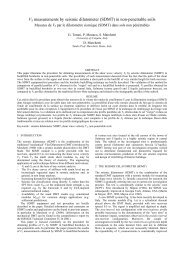
TC16 (2001) - Marchetti S., Monaco P., 

Totani G. & Calabrese M. "The Flat 

Dilatometer Test (DMT) in Soil Investigations" 

A Report by the ISSMGE Committee 

TC16. Proc. IN SITU 2001, Intnl. Conf. On 

In situ Measurement of Soil Properties, Bali, 

Indonesia, May 2001, 41 pp. 

ABSTRACT: This report presents an overview of the DMT equipment, testing procedure, interpretation and 

design applications. It is a statement on the general practice of dilatometer testing and is not intended to be a 

standard. 

FOREWORD 

This report on the flat dilatometer test is issued under 

the auspices of the ISSMGE Technical Committee 

TC16 (Ground Property Characterization from In- 

Situ Testing). It was authored by the Geotechnical 

Group of L'Aquila University with additional input 

from other members of the Committee. 

The first outline of this report was presented and 

discussed at the TC16 meeting in Atlanta – ISC '98 

(April 1998). The first draft was presented and 

discussed at the TC16 meeting in Amsterdam – 12 th 

ECSMGE (June 1999). 

Members of the Committee and practitioners were 

invited to review the draft and provide comments. 

These comments have been edited and taken into 

account by the original authors and incorporated in 

this report. 

AIMS OF THE REPORT 

This report describes the use of the flat dilatometer 

test (DMT) in soil investigations. The main aims of 

the report are: 

– To give a general overview of the DMT and of its 

design applications 

– To provide "state of good practice" guidelines for 

the proper execution of the DMT 

– To highlight a number of significant recent findings 

and practical developments. 

This report is not intended to be (or to originate in 

the near future) a Standard or a Reference Test 

Procedure (RTP) on DMT execution. 

Efforts have been made to preserve similarities in 

format with previous reports of the TC16 and other 

representative publications concerning in situ testing. 

The content of this report is heavily influenced by 

the experience of the authors, who are responsible for 

the facts and the accuracy of the data presented 

herein. 

Efforts have been made to keep the content of the 

report as objective as possible. 

Occasionally subjective comments, based on the 

authors experience, have been included when 

considered potentially helpful to the readers. 

SECTIONS OF THIS REPORT 

PART A – PROCEDURE AND OPERATIVE ASPECTS 

1. BRIEF DESCRIPTION OF THE FLAT 

DILATOMETER TEST 

2. DMT EQUIPMENT COMPONENTS 

3. FIELD EQUIPMENT FOR INSERTING THE 

DMT BLADE 

4. MEMBRANE CALIBRATION 

5. DMT TESTING PROCEDURE 

6. REPORTING OF TEST RESULTS 

7. CHECKS FOR QUALITY CONTROL 

8. DISSIPATION TESTS 

PART B – INTERPRETATION AND APPLICATIONS 

9. DATA REDUCTION AND INTERPRETATION 

10. INTERMEDIATE DMT PARAMETERS 

11. DERIVATION OF GEOTECHNICAL 

PARAMETERS 

12. PRESENTATION OF DMT RESULTS 

13. APPLICATION TO ENGINEERING 

PROBLEMS 

14. SPECIAL CONSIDERATIONS 

15. CROSS RELATIONS WITH RESULTS FROM 

OTHER IN SITU TESTS 

BACKGROUND AND REFERENCES 

BACKGROUND 

The flat dilatometer test (DMT) was developed in 

Italy by Silvano Marchetti. It was initially introduced 

in North America and Europe in 1980 and is 

currently used in over 40 countries. 

1

The DMT equipment, the test method and the 

original correlations are described by Marchetti 

(1980) "In Situ Tests by Flat Dilatometer", ASCE Jnl 

GED, Vol. 106, No. GT3. Subsequently, the DMT 

has been extensively used and calibrated in soil 

deposits all over the world. 

BASIC DMT REFERENCES / KEY PAPERS 

Various international standards and manuals are 

available for the DMT. An ASTM Suggested Method 

was published in 1986. A "Standard Test Method for 

Performing the Flat Plate Dilatometer" is currently 

being prepared by ASTM (approved Draft 2001). 

The test procedure is also standardized in the 

Eurocode 7 (1997). National standards have also 

been developed in various countries (e.g. Germany, 

Sweden). A comprehensive manual on the DMT was 

prepared for the United States Department of 

Transportation (US DOT) by Briaud & Miran in 

1992. Design applications and new developments are 

covered in detail in a state of the art report by 

Marchetti (1997). A list of selected comprehensive 

DMT references is given here below. 

STANDARDS 

ASTM Subcommittee D 18.02.10 - Schmertmann, J.H., 

Chairman (1986). "Suggested Method for Performing the 

Flat Dilatometer Test". ASTM Geotechnical Testing Journal, 

Vol. 9, No. 2, June. 

Eurocode 7 (1997). Geotechnical design - Part 3: Design 

assisted by field testing, Section 9: Flat dilatometer test 

(DMT). 

MANUALS 

Marchetti, S. & Crapps, D.K. (1981). "Flat Dilatometer 

Manual". Internal Report of G.P.E. Inc. 

Schmertmann, J.H. (1988). Rept. No. FHWA-PA-87-022+84- 

24 to PennDOT, Office of Research and Special Studies, 

Harrisburg, PA, in 4 volumes. 

US DOT - Briaud, J.L. & Miran, J. (1992). "The Flat 

Dilatometer Test". Departm. of Transportation - Fed. 

Highway Administr., Washington, D.C., Publ. No. FHWA- 

SA-91-044, 102 pp. 

STATE OF THE ART REPORTS 

Lunne, T., Lacasse, S. & Rad, N.S. (1989). "State of the Art 

Report on In Situ Testing of Soils". Proc. XII ICSMFE, Rio 

de Janeiro, Vol. 4. 

Lutenegger, A.J. (1988). "Current status of the Marchetti 

dilatometer test". Special Lecture, Proc. ISOPT-1, Orlando, 

Vol. 1. 

Marchetti, S. (1997). "The Flat Dilatometer: Design 

Applications". Proc. Third International Geotechnical 

Engineering Conference, Keynote lecture, Cairo University, 

28 pp. 

CONFERENCES, SEMINARS, COURSES 

Several conferences, seminars and courses have been 

dedicated to the DMT. The most important are 

mentioned here below. 

– First International Conference on the Flat Dilatometer, 

Edmonton, Alberta (Canada), Feb. 1983. 

– One-day Short Course on the DMT held by S. Marchetti in 

Atlanta (GA), USA, in connection with the First 

International Conference on Site Characterization (ISC '98), 

Apr. 1998. 

– International Seminar on "The Flat Dilatometer and its 

Applications to Geotechnical Design" held by S. Marchetti 

at the Japanese Geotechnical Society, Tokyo, Feb. 1999. 

DMT ON THE INTERNET 

Key papers on the DMT can be downloaded from the 

bibliographic site: http://www.marchetti-dmt.it 

PART A 

PROCEDURE AND OPERATIVE ASPECTS 

1. BRIEF DESCRIPTION OF THE FLAT 

DILATOMETER TEST 

The flat dilatometer is a stainless steel blade having a 

flat, circular steel membrane mounted flush on one 

side (Fig. 1). 

The blade is connected to a control unit on the 

ground surface by a pneumatic-electrical tube 

(transmitting gas pressure and electrical continuity) 

running through the insertion rods. A gas tank, 

connected to the control unit by a pneumatic cable, 

supplies the gas pressure required to expand the 

membrane. The control unit is equipped with a 

pressure regulator, pressure gage(s), an audio-visual 

signal and vent valves. 

Fig. 1. The flat dilatometer - Front and side view 

2

where the grains are small compared to the 

membrane diameter (60 mm). It is not suitable for 

gravels, however the blade is robust enough to cross 

gravel layers of about 0.5 m thickness. 

Due to the balance of zero pressure measurement 

method (null method), the DMT readings are highly 

accurate even in extremely soft - nearly liquid soils. 

On the other hand the blade is very robust (can safely 

withstand up to 250 kN of pushing force) and can 

penetrate even soft rocks. Clays can be tested from 

c u = 2-4 kPa up to 1000 kPa (marls). The range for 

moduli M is from 0.4 MPa up to 400 MPa. 

2. DMT EQUIPMENT COMPONENTS 

The basic equipment for dilatometer testing consists 

of the components shown in Fig. 2. 

Fig. 2. General layout of the dilatometer test 

The blade is advanced into the ground using common 

field equipment, i.e. push rigs normally used for the 

cone penetration test (CPT) or drill rigs. Push rods 

are used to transfer the thrust from the insertion rig 

to the blade. 

The general layout of the dilatometer test is shown 

in Fig. 2. The test starts by inserting the dilatometer 

into the ground. Soon after penetration, by use of the 

control unit, the operator inflates the membrane and 

takes, in about 1 minute, two readings: 

1) the A-pressure, required to just begin to move the 

membrane against the soil ("lift-off") 

2) the B-pressure, required to move the center of the 

membrane 1.1 mm against the soil. 

A third reading C ("closing pressure") can also 

optionally be taken by slowly deflating the membrane 

soon after B is reached. 

The blade is then advanced into the ground of one 

depth increment (typically 20 cm) and the procedure 

for taking A, B readings repeated at each depth. 

The pressure readings A, B are then corrected by 

the values ∆A, ∆B determined by calibration to take 

into account the membrane stiffness and converted 

into p 0 , p 1 . 

The field of application of the DMT is very wide, 

ranging from extremely soft soils to hard soils/soft 

rocks. The DMT is suitable for sands, silts and clays, 

2.1 DILATOMETER BLADE 

2.1.1 Blade and membrane characteristics 

The nominal dimensions of the blade are 95 mm 

width and 15 mm thickness. The blade has a cutting 

edge to penetrate the soil. The apex angle of the edge 

is 24° to 32°. The lower tapered section of the tip is 

50 mm long. The blade can safely withstand up to 

250 kN of pushing thrust. 

The circular steel membrane is 60 mm in diameter. 

Its normal thickness is 0.20 mm (0.25 mm thick 

membranes are sometimes used in soils which may 

cut the membrane). The membrane is mounted flush 

on the blade and kept in place by a retaining ring. 

2.1.2 Working principle 

The working principle of the DMT is illustrated in 

Fig. 3 (see also the photo in Fig. 4). The blade works 

as an electric switch (on/off). The insulating seat 

prevents electrical contact of the sensing disc with the 

underlying steel body of the dilatometer. The sensing 

disc is stationary and is kept in place press-fitted 

inside the insulating seat. The contact is signaled by 

an audio/visual signal. The sensing disc is grounded 

(and the control unit emits a sound) under one of the 

following circumstances: 

1) the membrane rests against the sensing disc (as 

prior to membrane expansion) 

2) the center of the membrane has moved 1.1 mm 

into the soil (the spring-loaded steel cylinder 

makes contact with the overlying sensing disc). 

There is no electrical contact, hence no signal, at 

intermediate positions of the membrane. 

When the operator starts increasing the internal 

pressure (Fig. 3), for some time the membrane does 

not move and remains in contact with its metal 

support (signal on). When the internal pressure 

3

Fig. 3. DMT working principle 

Fig. 4. Particular of the DMT blade 

counterbalances the external soil pressure, the 

membrane initiates its movement, losing contact with 

its support (signal off). The interruption of the signal 

prompts the operator to read the "lift-off" A-pressure 

(later corrected into p 0 ). The operator, without 

stopping the flow, continues to inflate the membrane 

(signal off). When the central movement reaches 1.1 

mm the spring-loaded steel cylinder touches (and 

grounds) the bottom of the sensing disc, reactivating 

the signal. The reactivation of the signal prompts the 

operator to read the "full expansion" B-pressure 

(later corrected into p 1 ). 

The top of the sensing disc carries a 0.05 mm feeler 

having the function to improve the definition of the 

lift-off of the membrane, i.e. the instant at which the 

electrical circuit is interrupted. 

The fixed-displacement system insures that the 

membrane expansion will be 1.10 mm ± 0.02 mm 

regardless of the care of the operator, who cannot 

vary or regulate such distance. Only calibrated quartz 

(once plexiglas) cylinders (height 3.90 ± 0.01 mm) 

should be used to insure accuracy of the prefixed 

movement. 

NOTE: Remarks on the DMT working principle 

– The membrane expansion is not a load controlled 

test - apply the load and observe settlement - but a 

displacement controlled test - fix the displacement 

and measure the required pressure. Thus in all soils 

the central displacement (and, at least 

approximately, the strain pattern imposed to the 

soil) is the same. 

– The membrane is not a measuring organ but a 

passive separator soil-gas. The measuring organ is 

the gage at ground surface. The accuracy of the 

measurements is that of the gage. The zero offset 

of the gage can be checked at any time, being at 

surface. A low range pressure gage can be used, 

e.g. in very soft soils, to increase accuracy to any 

desired level. 

– The method of pressure measurement is the 

balance of zero (null method), providing high 

accuracy. 

– The blade works as an electric switch (on/off), 

without electronics or transducers. 

– Given the absence of delicate or regulable 

components, no special skills are required to 

operate the DMT. 

2.2 CONTROL UNIT 

2.2.1 Functions and components 

The control unit on ground surface is used to 

measure the A, B (C) pressures at each test depth. 

The control unit (Fig. 5) typically includes two 

pressure gages, a pressure source quick connect, a 

quick connect for the pneumatic-electrical cable, an 

electrical ground cable connection, a galvanometer 

and audio buzzer signal (activated by the electric 

switch constituted by the blade) which prompt when 

to read the A, B (C) pressures, and valves to control 

gas flow and vent the system. 

Fig. 5. Control unit 

4

2.2.2 Pressure gages 

The two pressure gages, connected in parallel, have 

different scale ranges: a low-range gage (1 MPa), 

self-excluding when the end of scale is reached, and a 

high-range gage (6 MPa). The two-gage system 

ensures proper accuracy and, at the same time, 

sufficient range for various soil types (from very soft 

to very stiff). 

According to Eurocode 7 (1997), the pressures 

should be measured with a resolution of 10 kPa and a 

reproducibility of 2.5 kPa, at least for pressures lower 

than 500 kPa. Gages should have an accuracy of at 

least 0.5 % of span. 

In case of discrepancy between the two gages, 

replace the malfunctioning gage or correct as 

appropriate. In case of single-gage (old control 

units), the gage should be periodically calibrated. 

Though the control unit is encased in an aluminium 

carrying case, it should be handled with care to avoid 

damaging the gages. 

2.2.3 Gas flow control valves 

The valves on the control unit panel permit to control 

the gas flow to the blade. 

The main valve provides a positive shutoff between 

the gas source and the blade-control unit system. The 

micrometer flow valve is used to control the rate of 

flow during the test. It also provides a shutoff 

between the source and the DMT system (anyway it 

is advisable to close the main valve and to open the 

toggle vent valve if the control unit is left unattended 

for some time). The toggle vent valve allows the 

operator to vent quickly the system pressure to the 

atmosphere. The slow vent valve allows to vent the 

system slowly for taking the C-reading. 

2.2.4 Electrical circuit 

The electrical circuitry in the control unit has the 

scope of indicating the on/off condition of the bladeswitch. 

It provides both a visual galvanometer and an 

audio buzzer signal to the operator. The buzzer is on 

when the blade is in the short circuit condition, i.e. 

collapsed against the blade or fully expanded. The 

buzzer is off when between these two positions. The 

transitions from buzzer on to off and then off to on as 

the membrane expands are the prompts for the 

operator to take respectively the A and B pressure 

readings. 

A 9-Volt battery supplies electrical power to the 

wire inside the pneumatic-electrical cable quickconnect. 

The power is returned at the ground cable 

jack if the blade is in the short circuit condition. 

A test button permits to check the vitality of the 

battery and the operation of the galvanometer and 

buzzer. Note that it simply shorts across the blade 

portion of the circuit and hence provides no 

information about the status of the blade, the 

pneumatic-electrical cable or the ground cable. If 

annoyed by the sound during test delays, the operator 

may disable the buzzer. However, quieting the buzzer 

involves the risk of missing the prompts to take the 

readings and overinflating the membrane. 

2.3 PNEUMATIC-ELECTRICAL CABLE 

The pneumatic-electrical (p-e) cable provides 

pneumatic and electrical continuity between the 

control unit and the dilatometer blade. It consists of a 

stainless steel wire enclosed within nylon tubing with 

special metal connectors at either end. Two different 

cable types are normally used (Fig. 6): 

– Non-extendable cable: this cable has an insulated 

male metal connector for the DMT blade on one 

end, and a non-insulated quick-connect for 

attachment to the control unit on the other end. 

The cable length (minus a working length at the 

surface) limits the maximum sounding depth: once 

the test depth is such that all the cable is inside the 

soil, the cable cannot be extended and the test must 

be stopped. This inconvenience is balanced by the 

simplicity of the cable and its lower cost. 

– Extendable cable: by using an extendable cable, 

the operator may connect additional cable(s) as 

needed during the sounding. The female terminal of 

such cable (insulated) cannot fit directly into the 

corresponding quick connector in the control unit. 

Therefore a cable leader (or short connector 

cable) permitting such a connection must be used 

in conjunction with this cable. This short adaptor is 

removed when a new cable is added. Though 

slightly more complex, this type of cable provides 

the operator with greater flexibility. 

The proper type and length of cable should be chosen 

based on the expected sounding depth. For ease of 

handling and to minimize pressure lag at the control 

unit gage, always use the shortest length practical. 

Fig. 6. Types of pneumatic-electrical cables 

5

Short cables are easier to handle, but require 

junctions. Junctions normally work well and do not 

represent a problem as long as care is exercised to 

avoid particles of soils getting into the conduits. 

To keep contaminants out, the terminals and 

connectors must always be protected with caps when 

disconnected. 

The metal connectors are electrically insulated from 

the inner wire to prevent a short circuit in the ground 

and sealed by washers to prevent gas leakage. 

The cables and terminals are not easily repairable in 

the field. 

2.4 GAS PRESSURE SOURCE 

The pressure source is a gas tank equipped with a 

pressure regulator, valves and pneumatic tubing to 

connect to the control unit. 

The pressure regulator (suitable to gas type) must 

be able to supply a regulated output pressure of at 

least 7-8 MPa. 

When testing in most soils the output pressure is set 

at 3-4 MPa. In very hard soils the output pressure is 

further increased (without exceeding the high-range 

gage capacity). 

Any non flammable, non corrosive, non toxic gas 

may be used. Compressed nitrogen or compressed air 

(scuba tanks) are most generally used. 

Gas consumption increases with applied pressure 

(A, B readings) and test depth (cable length). In 

"average" soils a scuba size tank (≈ 0.6 m high), 

initially at 15 MPa, contains gas to perform 

approximately 70-100 m of "standard" sounding (≈ 

one day of testing). In general, it is more economical 

and efficient to have a large tank (≈ 1.5 m high) when 

more than one day of testing is anticipated. 

2.5 ELECTRICAL GROUND CABLE 

The ground cable provides electrical continuity 

between the push rods and the control unit. It returns 

to the control unit the simple on/off electrical power 

carried to the blade by the pneumatic-electrical cable. 

3. FIELD EQUIPMENT FOR INSERTING 

THE DMT BLADE 

3.1 PUSHING EQUIPMENT 

The dilatometer blade is advanced into the ground 

using common field equipment. 

The blade can be pushed with a cone penetrometer 

rig or with a drill rig (Fig. 7). 

The penetration rate is usually 2 cm/s as in the CPT 

(for DMT rates from 1 to 3 cm/s are acceptable, see 

Eurocode 7 1997). 

DMT USING A 

PENETROMETER 

DMT USING A 

DRILL RIG 

Fig. 7. Equipment for inserting the DMT blade 

The DMT can also be driven, e.g. using the SPT 

hammer and rods, but statical push is by far 

preferable. 

Heavy truck-mounted penetrometers are 

incomparably more efficient than drill rigs. Moreover 

the soil provides lateral support to the rods (which is 

not the case in a borehole). Pushing the blade with a 

20 ton penetrometer truck is most effective and yields 

the highest productivity (up to 80 m of sounding per 

day). 

Drill rigs or light rigs may be used only in soft soils 

or to very short depths. In all other cases (especially 

in hard soils) light rigs may be inadequate and source 

of problems. However drill rigs may be necessary in 

soils containing occasional boulders or hard layers, 

where the obstacle-destroying capability will permit 

to continue the test past the obstacle. 

When the DMT sounding is resumed after 

preboring, the initial test results, obtained in the zone 

of disturbance at hole bottom (≈ 3 to 5 borehole 

diameters), should be regarded with caution. 

When the DMT is performed inside a borehole, the 

diameter of the borehole (and casing, if required) 

should be as small as possible to minimize the risk of 

buckling (possibly 100-120 mm). 

In all cases the penetration must occur in "fresh" 

(not previously penetrated) soil. The minimum 

recommended distance from other nearby DMT (or 

CPT) soundings is 1 m (25 diameters from 

unbackfilled/uncased borings). 

6

NOTE: Possible problems with light rigs 

Possible problems with light rigs (such as many SPT 

rigs) are: 

– Light rigs have typically a pushing capacity of only 

2 tons, hence refusal is found very soon (often at 

1-2 m depth). 

– Often there is no collar near ground surface (i.e. no 

ground surface side-guidance of the rods). 

– There is a hinge-type connection in the rods just 

below the pushing head, which permits excessive 

freedom and oscillations of the rods inside the hole. 

– The distance between the pushing head of the rig 

and the bottom of the hole is several meters, hence 

the free/buckling length of the rods is high. In some 

cases the loaded rods have been observed to 

assume a "Z" shape. 

– Oscillations of the rods may cause wrong results. 

In case of short penetration in hard layers it was 

occasionally observed that the "Z" shape of the 

rods suddenly reverted to the opposite side. This is 

one of the few cases in which the DMT readings 

may be instrumentally incorrect: oscillations of the 

rods cause tilting of the blade, and the membrane is 

moved without control close to/far from the soil. 

NOTE: Pushing vs driving 

Various researchers (US DOT 1992, Schmertmann 

1988) have observed that "hammer-driving alters the 

DMT results and decreases the accuracy of 

correlations", i.e. the insertion method does affect the 

test results, and static penetration should be 

preferred. 

According to ASTM (1986), in soils sensitive to 

impact and vibrations, such as very loose sand or 

very sensitive clays, dynamic insertion methods can 

significantly change the test results compared to 

those obtained using a static push. In general, 

structurally sensitive soils will appear conservatively 

more compressible when tested using dynamic 

insertion methods. In such cases the engineer may 

need to check such dynamic effects and, possibly, 

calibrate and adjust test interpretation accordingly. 

US DOT (1992) recommends that, if the driving 

technique is used, as a minimum 2 soundings be 

performed side by side, one by pushing and one by 

driving. This would give a site/soil specific 

correlation, which would allow to get back to the 

parameters obtained from correlations based on the 

pushing insertion (with added imprecision, however). 

According to Eurocode 7 (1997), driving should be 

avoided except when advancing the blade through 

stiff or strongly cemented layers which cannot be 

penetrated by static push. 

3.2 PUSH RODS 

While in principle any kind of rod can be used, most 

commonly CPT rods or drill rig rods are employed. 

A friction reducer is sometimes used. However the 

consequent reduction in rod friction is moderate, 

because of the multi-lobate shape of the cavity 

produced in the penetrated soil by the blade-rod 

system. 

If used, the friction reducer should be located at 

least 200 mm above the center of the membrane 

(Eurocode 7 1997). 

NOTE: Use of stronger rods 

Many heavy penetrometer trucks performing DMT 

are today also equipped with rods much stronger than 

the common 36 mm CPT rods. Such stronger rods 

are typically 44 to 50 mm in diameter, 1 m length, 

same steel as CPT rods (yield strength > 1000 MPa). 

A very suitable and convenient type of rod is the 

commercially available 44 mm rod used for pushing 

15 cm 2 cones. 

The stronger rods have been introduced since the 

rods are "the weakest element in the chain" when 

working with heavy trucks and the current high 

strength DMT blades, able to withstand a working 

load of approximately 250 kN. 

The stronger rods have several advantages: 

– Capability of penetrating through cemented 

layers/obstacles. 

– Better lateral stability against buckling in the first 

few meters in soft soils or when the rods are 

pushed inside an empty borehole. 

– Possibility of using completely the push capacity of 

the truck. 

– Reduced risk of deviation from the verticality in 

deep tests. 

– Drastically reduced risk of loosing the rods. 

Obvious drawbacks are the initial cost and the 

heavier weight. Also, their use may not be convenient 

in OC clay sites because of the increased skin friction. 

3.3 ROD ADAPTORS 

The DMT blade is connected to the push rods by a 

lower adaptor (Fig. 8). 

The most common adaptor has its top connectable 

to CPT rods, its bottom connectable to the DMT 

blade (ending cylindrical male M27x3mm). 

If rods other than CPT rods are used, specific 

adaptors need to be prepared (see Fig. 8). 

An upper slotted adaptor is also needed to allow 

lateral exit of cable, otherwise pinched by the pushing 

head. 

7

(a) 

Fig. 8. Lower adaptor connecting the DMT blade 

to the push rods 

When using a CPT truck, a DMT sounding normally 

starts from the ground surface, with the tube running 

inside the rods (Fig. 9a, left). 

When testing starts from the bottom of a borehole, 

the pneumatic-electrical (p-e) cable can either run all 

the way up inside the rods, or can exit laterally from 

the rods at a suitable distance above the blade (Fig. 

9a, right). In this case an additional intermediate 

slotted adaptor is needed to permit egress of the 

cable (Fig. 9a, right). Above this point the cable is 

taped to the outside of the rods at 1-1.5 m intervals 

up to the surface. 

The torpedo-like bottom assembly in Fig. 9a is 

composed by the blade, 3 to 5 m (generally) of rods 

and the intermediate slotted adaptor. The "torpedo" 

is pre-assembled and then mounted at the end of the 

rods each time. The "torpedo" arrangement speeds 

production, since it is easier to handle the upper rods 

free from the cable. 

Since the unprotected cable is vulnerable, the 

intermediate slotted adaptor needs a special collar 

(Fig. 9b). The collar has a vertical channel for the 

cable and has a diameter larger than the upper rods so 

as to insure a free space between the upper rods and 

the casing. The operator should not allow the slotted 

adaptor and the exposed cable to penetrate the soil, 

thus limiting the test depth to the length of rods 

threaded at the bottom. 

4. MEMBRANE CALIBRATION 

4.1 DEFINITIONS OF DA AND DB 

The calibration procedure consists in obtaining the 

∆A and ∆B pressures necessary to overcome 

(b) 

Fig. 9. (a) Possible exits of the cable from the rods 

(b) Intermediate slotted adaptor joining the 

upper push rods to the torpedo-like bottom 

assembly of blade and rods 

membrane stiffness. ∆A and ∆B are then used to 

correct the A, B readings. 

Note that in air, under atmospheric pressure, the 

free membrane is in an intermediate position between 

the A and B positions, because the membranes have a 

slight natural outward curvature (Fig. 10). 

∆A is the external pressure which must be applied 

to the membrane, in free air, to collapse it against its 

seating (i.e. A-position). ∆B is the internal pressure 

which, in free air, lifts the membrane center 1.1 mm 

from its seating (i.e. B-position). 

Various aspects related to the membrane calibration 

are described in detail by Marchetti (1999) and 

Marchetti & Crapps (1981). 

8

free 

Fig. 10. Positions of the membrane (free, A and B) 

NOTE: Meaning of the term "calibration" 

The membrane calibration is not, strictly speaking, a 

calibration, since the term calibration usually refers 

to the scale of a measuring instrument. The 

membrane, instead, is a passive separator gas/soil and 

not a measuring instrument. Actually the membrane is 

a "tare" and the "calibration" is in reality a "tare 

determination". 

4.2 DETERMINATION OF DA AND DB 

∆A and ∆B can be measured by a simple procedure 

using a syringe to generate vacuum or pressure. 

During the calibration the high pressure from the 

bottle should be excluded from the pneumatic circuit 

by closing the main valve on the control unit panel. 

To obtain ∆A: quickly pull back (almost fully) the 

piston of the syringe, in order to apply the maximum 

vacuum possible (the vacuum causes an inward 

deflection of the membrane similar to that resulting 

from the external soil pressure at the start of the test). 

Hold the piston for sufficient time (at least 5 seconds) 

for the vacuum to equalize in the system. During this 

time the buzzer signal should become active. Then 

slowly release the piston and read ∆A on the lowrange 

gage (gage vacuum reading at which the buzzer 

stops, i.e. A-position). Note this negative pressure as 

a positive ∆A value (e.g. a vacuum of 15 kPa should 

be reported as ∆A = 15 kPa). The correction formula 

for p 0 (Eq. 1 in Section 9.2) is already adjusted to 

take into account that a positive ∆A is a vacuum. 

To obtain ∆B: push slowly the piston into the 

syringe and read ∆B on the low-range gage when the 

buzzer reactivates (i.e. B-position). 

Repeat this procedure several times to have a 

positive check of the values being read. 

Membrane corrections ∆A, ∆B should be measured 

before a sounding, after a sounding, whenever the 

blade is removed from the ground. 

∆A, ∆B are usually measured, as a check, in the 

office before moving to the field. However the initial 

∆A, ∆B to be used are those taken just before the 

sounding (though the difference is generally 

negligible). The final values of ∆A, ∆B must also be 

taken at the end of the sounding. 

The calibration values of an undamaged membrane 

remain relatively constant during a DMT sounding. 

Comparison of before/after values indicates the 

B 

A 

condition of the membrane and a large difference 

should prompt a membrane change. Therefore, the 

calibration procedure is a good indicator of the 

equipment condition, and consequently of the 

expected quality of the data. 

4.3 ACCEPTANCE VALUES OF DA AND DB 

Acceptance values of ∆A, ∆B are indicated in 

Eurocode 7 (1997). 

– The initial ∆A, ∆B values must be in the following 

ranges: ∆A = 5 to 30 kPa, ∆B = 5 to 80 kPa. If the 

values of ∆A, ∆B obtained before inserting the 

blade into the soil fall outside the above limits, the 

membrane shall be replaced before testing. 

– The change of ∆A or ∆B at the end of the sounding 

must not exceed 25 kPa, otherwise the test results 

shall be discarded. 

Typical values of ∆A, ∆B are: ∆A = 15 kPa, ∆B = 40 

kPa. 

∆A, ∆B values also indicate when it is time to 

replace a membrane. An old membrane needs not to 

be replaced as long as ∆A, ∆B are in tolerance. 

Indeed an old membrane is preferable, in principle, 

to a new one, having more stable and lower ∆A, ∆B. 

However, in case of bad wrinkles, scratches, etc. a 

membrane should be changed even if ∆A, ∆B are in 

tolerance (though ∆A, ∆B are not likely to be in 

tolerance if the membrane is in a really bad shape). 

4.4 CONFIGURATIONS DURING THE CALIBRATION 

The membrane calibration (determining ∆A, ∆B) can 

be performed in two configurations. 

1) The first configuration (blade accessible, Fig. 11) 

is adopted e.g. at the beginning of a sounding, 

when the blade is still in the hands of the operator. 

Fig. 11. Layout of the connections during 

membrane calibration (blade accessible) 

9

The operator will then use the short calibration 

cable, or the short calibration connector. 

2) The second configuration (blade not readily 

accessible) is used when the blade is under the 

penetrometer, and is connected to the control unit 

as during current testing (Fig. 12) with cables of 

normal length (say 20 to 30 m). 

The calibration procedure is the same. The only 

difference is that, in the second case, due to the 

length of the DMT tubings, there is some time lag 

(easily recognizable by the slow response of the 

pressure gages to the syringe). Therefore, in that 

configuration, ∆A, ∆B must be taken slowly (say 15 

seconds for each determination). 

4.5 EXERCISING THE MEMBRANE 

The exercising operation is to be performed 

whenever a new membrane is mounted. A new 

membrane needs to be "exercised" in order to 

stabilize ∆A, ∆B values (obtain ∆A, ∆B values which 

will remain constant during the sounding). 

The exercising operation simply consists in 

pressurizing the blade in free air at about 500 kPa for 

a few seconds two or three times. 

If the membrane exercising is performed with the 

blade submerged in water, it is possible to verify 

blade airtightness. 

After exercising, verify that ∆A, ∆B are in 

tolerance: ∆A = 5 to 30 kPa (typically 15 kPa), ∆B = 

5 to 80 kPa (typically 40 kPa). 

4.6 IMPORTANCE OF ACCURATE DA AND DB 

The importance of accurate ∆A, ∆B measurements, 

especially in soft soils, is pointed out by Marchetti 

(1999). Inaccurate ∆A, ∆B are virtually the only 

potential source of DMT instrumental error. Since 

∆A, ∆B are used to correct all A, B of a sounding, 

any inaccuracy in ∆A, ∆B would propagate to all the 

data. 

The importance of ∆A, ∆B in soft soils derives from 

the fact that, in the extreme case of nearly liquid 

clays, or liquefiable sands, A and B are small 

numbers, just a bit higher than ∆A, ∆B. Since the 

correction involves differences between similar 

numbers, accurate ∆A, ∆B are necessary in such soils. 

∆A, ∆B must be, as a rule, measured before and 

after each sounding. Their average is subsequently 

used to correct all A, B readings. Clearly, if the 

variation is small, the average represents ∆A, ∆B 

reasonably well at all depths. If the variation is large, 

the average may be inadequate at some depths. In 

fact, in soft soils, the operator can be sure that the 

test results are acceptable only at the end of the 

sounding, when, checking ∆A, ∆B final, he finds that 

they are very similar to ∆A, ∆B initial. 

In medium to stiff soils ∆A, ∆B are a small part of A 

and B, so small inaccuracies in ∆A, ∆B have 

negligible effect. 

NOTE: How ∆A, ∆B can go out of tolerance 

In practice the only mechanism by which ∆A, ∆B can 

go out of tolerance is overinflating the membrane far 

beyond the B-position. Once overinflated, a 

membrane requires excessive suction to close (∆A 

generally > 30 kPa), and even ∆B may be a suction. 

5. DMT TESTING PROCEDURE 

5.1 PRELIMINARY CHECKS AND OPERATIONS 

BEFORE TESTING 

Select for testing only blades respecting the 

tolerances (have available at least two). Similarly, use 

only properly checked pieces of equipment. 

Pre-thread the pneumatic-electrical (p-e) cable 

through a suitable number of push rods and the 

adaptors. During this operation keep the cable 

terminals protected from dirt with the caps. 

Wrench-tighten the cable terminal to the blade. 

Connect the blade to the bottom push rod (with 

interposed the lower adaptor). Avoid excessive twists 

in the cable while making the connections. 

Insert the electrical ground cable plug into the 

"ground" jack of the control unit. Clip the other end 

(electrical alligator clip) to the upper slotted adaptor 

or to one of the push rods (not to the metal frame of 

the rig, which may be not in firm electrical contact 

with the rods). 

The connections should be as indicated in Fig. 12 

(but do not open the valve of the bottle yet!). 

Fig. 12. Layout of the connections during current 

testing 

10

Check the electrical continuity and the switch 

mechanism by pressing the center of the membrane. 

The signal should activate. If not, make the 

appropriate repair. 

Record the zero of the gage Z M (reading of the gage 

for zero pressure) by opening the toggle vent valve 

and read the pressure while tapping gently on the 

glass of the gage. 

Perform the calibration as described in detail in 

Section 4. 

With the gas tank valve closed, connect the 

pressure regulator to the tank and set the regulated 

pressure to zero (fully unscrew the regulating lever). 

Connect the pneumatic cable from the gas tank 

regulator to the control unit female quick connector 

marked "pressure source". 

Make sure that: the main valve is closed, the toggle 

vent valve is open and the micrometer flow valve is 

closed. 

Set the regulator so that the pressure supplied to 

the control unit is about 3 MPa (this pressure can be 

later increased if necessary). Open the tank valve. 

Open the main valve. (This valve normally remains 

always open during current testing. During current 

testing the operator only uses the micrometer flow 

valve and the vent valves). 

5.2 STEP-BY-STEP TEST PROCEDURE (A, B, C 

READINGS) 

The DMT test basically consists in the following 

sequence of operations. 

1) The DMT operator makes sure that the 

micrometer flow valve is closed and the toggle 

vent valve open, then he gives the go-ahead to the 

rig operator (the two operators should position 

themselves in such a way they can exchange 

control and visual communication easily). 

2) The rig operator pushes the blade vertically into 

the soil down to the selected test depth, either 

from ground surface or from the bottom of a 

borehole. During the advancement the signal 

(galvanometer and buzzer) is normally on because 

the soil pressure closes the membrane. (The signal 

generally starts at 20 to 40 cm below ground 

surface). 

3) As soon as the test depth is reached, the rig 

operator releases the thrust on the push rods and 

gives the go-ahead to the DMT operator. 

4) The DMT operator closes the toggle vent valve 

and slowly opens the micrometer flow valve to 

pressurize the membrane. During this time he 

hears a steady audio signal or buzzer on the 

control unit. At the instant the signal stops (i.e. 

when the membrane lifts from its seat and just 

begins to move laterally), the operator reads the 

pressure gage and records the first pressure 

reading A. 

5) Without stopping the flow, the DMT operator 

continues to inflate the membrane (signal off) until 

the signal reactivates (i.e. membrane movement = 

1.1 mm). At this instant the operator reads at the 

gage the second pressure reading B. After 

mentally noting or otherwise recording this value, 

he must do the following four operations: 

1 - Immediately open the toggle vent valve to 

depressurize the membrane. 

2 - Close the micrometer flow valve to prevent 

further supply of pressure to the dilatometer 

(these first two operations prevent further 

expansion of the membrane, which may 

permanently deform it and change its 

calibrations, and must be performed quickly 

after the B-reading, otherwise the membrane 

may be damaged). 

3 - Give the rig operator the go-ahead to advance 

one depth increment - generally 20 cm (the 

toggle vent valve must remain open during 

penetration to avoid pushing the blade with 

the membrane expanded). 

4 - Write the second reading B. 

Repeat the above sequence at each depth until the 

end of the sounding. At the end of the sounding, 

when the blade is extracted, perform the final 

calibration. 

If the C-reading is to be taken, there is only one 

difference in the above sequence. In Step 5.1, after B, 

open the slow vent valve instead of the fast toggle 

vent valve and wait (approximately 1 minute) until 

the pressure drops approaching the zero of the gage. 

At the instant the signal returns take the C-reading. 

Note that, in sands, the value to be expected for C 

is a low number, usually < 100 - 200 kPa, i.e. 10 or 

20 m of water. 

NOTE: Frequent mistake in C-readings 

As remarked in DMT Digest Winter 1996 (edited by 

GPE Inc., Gainesville, Florida), several users have 

reported poor C-readings, mostly due to improper 

technique. The frequent mistake is the following. 

After B, i.e. when the slow deflation starts, the signal 

is on. After some time the signal stops (from on to 

off). The mistake is to take the pressure at this 

inversion as C, which is incorrect (at this time the 

membrane is the B-position). The correct instant for 

taking C is some time later, when, completed the 

deflation, after say 1 minute, the membrane returns to 

the "closed" A-position, thereby contacting the 

supporting pedestal and reactivating the signal. 

11

NOTE: Frequence of C-readings 

(a) Sandy sites 

In sands (B ≥ 2.5 A) C-readings may be taken 

sporadically, say every 1 or 2 m, and are used to 

evaluate u 0 (equilibrium pore pressure). It is advisable 

to repeat the A-B-C cycle several times to insure that 

all cycles provide similar C-readings. 

(b) Interbedded sands and clays 

If the interest is limited to finding the u 0 profile, then 

C-readings are taken in the sandy layers (B ≥ 2.5 A), 

say every 1 or 2 m. 

When the interest, besides u 0 , is to discern freedraining 

layers from non free-draining layers, then C- 

readings are taken at each test depth. 

NOTE: Electrical connections during testing 

The rig operator should never disconnect the ground 

cable (e.g. to add a rod which requires to remove the 

electrical alligator) while the DMT operator is taking 

the readings and anyway not before his go-ahead 

indication. 

NOTE: Expansion rate 

Pressures A and B must be reached slowly. 

According to the Eurocode 7 (1997), the rate of 

gas flow to pressurize the membrane shall be such 

that the A-reading is obtained (typically in 15 

seconds) within 20 seconds from reaching the test 

depth and the B-reading (expansion from A to B) 

within 20 seconds after the A-reading. As a 

consequence, the rate of pressure increase is very 

slow in weak soils and faster in stiff soils. 

The above time intervals typically apply for cables 

lengths up to approximately 30 m. For longer cables 

the flow rate may have to be reduced to allow 

pressure equalization along the cable. 

During the test, the operator may occasionally 

check the adequacy of the selected flow rate by 

closing the micrometer flow valve and observing how 

the pressure gage reacts. If the gage pressure drops in 

excess of 2 % when closing the valve (ASTM 1986), 

the rate is too fast and must be reduced. 

NOTE: Time required for the test 

The time delay between end of pushing and start of 

inflation is generally 1-2 seconds. The complete test 

sequence (A, B readings) generally requires about 1 

minute. The total time needed for obtaining a 

"typical" 30 m profile (if no obstructions are found) is 

about 3 hours. The C-reading adds about 45 seconds 

to 1 minute to the time required for the DMT 

sequence at each depth. 

NOTE: Depth increment 

A smaller depth increment (typically 10 cm) can be 

assumed, even limited to a single portion of the DMT 

sounding, whenever more detailed soil profiling is 

required. 

NOTE: Test depths 

The test depths should be recorded with reference to 

the center of the membrane. 

NOTE: Thrust measurement 

Some Authors or existing standards (Schmertmann 

1988, ASTM 1986, ASTM Draft 2001) recommend 

the measurement of the thrust required to advance 

the blade as a routine part of the DMT testing 

procedure. The specific aim of this additional 

measurement is to obtain q D (penetration resistance 

of the blade tip). q D permits to estimate K 0 and Φ in 

sand according to the method formulated by 

Schmertmann (1982, 1983). 

Measuring q D directly is highly impractical. One 

way of obtaining q D is to derive it from the thrust 

force, measurable by a properly calibrated load cell. 

The preferable location of such load cell would be 

immediately above the blade to exclude the rod 

friction (however the lateral friction on the blade has 

still to be detracted). Even this cell location is 

impractical and not presently adopted except for 

research purposes, so that the load cell is generally 

located above the ground surface. 

Practical alternative methods for estimating q D are 

indicated in ASTM (1986): (a) Measure the thrust at 

the ground surface and subtract the estimated 

parasitic rod friction above the blade. (b) Measure the 

thrust needed for downward penetration and the pull 

required for upward withdrawal: the difference gives 

an estimate of q D . (c) If values of the cone 

penetration resistance q c from adjacent CPT are 

available, assume q D ≈ q c (e.g. ASTM 1986, 

Campanella & Robertson 1991, ASTM Draft 2001). 

6. REPORTING OF TEST RESULTS 

("FIELD RAW DATA") 

A typical DMT field data form is shown in Fig. 13. 

Besides the field raw data, the test method should 

be described, or the reference to a published standard 

indicated. 

7. CHECKS FOR QUALITY CONTROL 

7.1 CHECKS ON HARDWARE 

7.1.1 Blade 

Membrane corrections tolerances 

Verify that all blades available at the site are within 

tolerances (initial ∆A = 5 to 30 kPa, initial ∆B = 5 to 

80 kPa). 

12

Fig. 13. Typical DMT field data form - (1 bar = 100 kPa) 

13

Sharpness of electrical signal 

Using the syringe (in the calibration configuration) 

apply 10 or more cycles of vacuum-pressure to verify 

sharpness of the electrical signal at the off and on 

inversions. If the signal inversions are not sharp, the 

likely reason is dirt between the contacts and the 

blade must be disassembled and cleaned. 

Airtightness 

Submerge the blades under water and pressurize 

them at 0.5 MPa. 

Elevations of sensing disc, feeler and quartz (once 

plexiglas) cylinder 

These checks are executed using a special "tripod" 

dial gage (Fig. 14). The legs of the tripod rest on the 

surrounding plane and the dial gage permits to 

measure the elevations above this plane. Their values 

should fall within the following tolerances: 

Sensing disc - Nominal elevation above the 

surrounding plane: 0.05 mm. Tolerance range: 0.04- 

0.07 mm. 

Feeler - Nominal elevation above the sensing disc: 

0.05 mm. Tolerance range: 0.04-0.07 mm. 

Quartz cylinder - Only calibrated quartz (once 

plexiglas) cylinders (height 3.90 ± 0.01 mm) should 

be used to insure accuracy of the prefixed movement. 

Therefore checking the elevation of the top of the 

quartz cylinder is redundant. However such elevation 

can be checked, and should be in the range 1.13-1.18 

mm above the membrane support plane. 

Sensing disc extraction force (the sensing disc must 

be stationary inside the insulating seat) 

The disc should fit tightly, thanks to the lateral 

gripping force, inside the insulating seat. The 

extraction force should be, as a minimum, equal to 

the weight of the blade so that, if the sensing disc is 

lifted, the blade is lifted too without falling. 

If the coupling becomes loose (disc free to move) 

then the gripping force should be increased. One 

quick fix can be the insertion, while reinstalling the 

disc, of a small piece of plastic sheet laterally (not on 

the bottom). 

Conditions of the penetration edge 

In case of severe denting of blade's edge, straighten 

the major undulations, then sharpen the edge using a 

file. 

Coaxiality between blade and axis of the rods 

With the lower adaptor mounted on the blade, place 

the inside edge of an L-square against the side of the 

adaptor. Note the distance from the penetration edge 

of the blade to the side of the L-square. Turn the 

Fig. 14. "Tripod" dial gage 

blade 180° and repeat the measurement. The 

difference between the two distances should not 

exceed 3 mm (corresponding to a coaxiality error of 

1.5 mm). 

Blade planarity 

Place a 15 cm ruler against the face of the blade 

parallel to its long side. The "sag" between the ruler 

and blade should not exceed 0.5 mm (to be checked 

with a flat 0.5 mm feeler gage). 

Check the blade for electrical continuity 

If the calibration has been carried out without 

irregularities in the expected electrical signal, the 

calibration itself already proves that the electrical 

function of the blade is working properly. 

Additional electrical checks can be carried out with 

the membrane removed (but with the quartz cylinder 

in its place) using a continuity tester. The open blade 

should respond electrically as follows: 

– Continuity between the metal tubelet and the 

sensing disc 

– Continuity between the metal tubelet and blade 

body if the quartz cylinder is lifted 

– No continuity (insulation) between the metal 

tubelet and blade body if the quartz cylinder is 

depressed (continuity in this case would mean that 

the blade is in short circuit). 

A recommended check just before mounting the 

membrane is the following: 

– Press 10 times or more on the quartz cylinder to 

insure that the on and off signal inversions are 

sharp and prompt. 

Sensing disc, underlying cavity and elements inside 

cavity must be perfectly clean 

The parts of the instrument inside the membrane 

(disc, spring, metal cylinder, cylinder housing) must 

be kept perfectly clean (e.g. blowing each piece with 

compressed air) to insure proper electrical contacts. 

14

Fig. 15. Electrical contact points to be kept clean 

to avoid membrane overinflation 

A complete guide for disassembling and cleaning the 

blade can be found in Marchetti & Crapps (1981) and 

Schmertmann (1988). 

In particular, the critical electrical contact points 

(highlighted in Fig. 15) should be perfectly free from 

dirt/grains/tissue. If not, the defective electrical 

contact will cause severe and costly inconveniences. 

In fact electrical malfunctioning will result in no B- 

signal. In absence of B-signal, the operator will keep 

inflating, eventually overexpanding the membrane 

beyond ∆A, ∆B tolerances, in which case the test 

results will be rejected. 

The risk of absence of B-reading can be reduced by 

the following check: before starting a sounding, 

repeat the calibration (∆A, ∆B) 10 times or more, to 

make sure that the B-signal is regular and sharp. 

7.1.2 Control unit 

Check the control unit for electrical operation 

– Press the test button with the audio switch on. The 

galvanometer and buzzer should activate. 

– Connect with a wire the inside of the "ground" jack 

with the female quick connector marked 

"dilatometer". The galvanometer and buzzer should 

activate. 

Check the control unit for gas leakage 

Close the vent valves, open the main valve and the 

micrometer flow valve. Pressurize the control unit to 

the maximum gage range. Close the main valve to 

avoid further pressure supply. Observe the gages for 

leaks. 

7.1.3 Pneumatic-electrical cables 

Check the cables for mechanical integrity 

Inspect the entire length to determine if the tubing is 

pinched or broken. 

Check the cables for electrical operation 

Check by a continuity tester both electrical continuity 

and electrical insulation between the terminals. 

The male quick connectors should be in contact with 

the inner wire, while the metal terminals should be 

insulated from the wire. 

Check the cables for gas leakage 

Plug with the special female closed-ended terminal 

the blade terminal of the cable and connect the other 

end of the cable to the control unit. Use the control 

unit to pressurize the cable to 4-6 MPa. Then close 

the micrometer flow valve. Observe the gage for any 

loss in pressure. A leak can be localized by immersing 

the cable and fittings in water. 

7.2 CHECKS ON TEST EXECUTION 

– Verify that A is reached in ≈ 15 seconds (within 20 

seconds), B in ≈ 15 seconds (within 20 seconds) 

after A. 

– The change of ∆A or ∆B before/after the sounding 

must not exceed 25 kPa, otherwise the test will be 

rejected. 

– The C-reading, when taken, should be obtained in 

45 to 60 seconds after starting the deflation 

following B. 

NOTE: Accuracy of DMT measurements 

The prefixed displacement is the difference between 

the height of the quartz (once plexiglas) cylinder and 

the thickness of the sensing disc. These components 

are machined to 0.01 mm tolerance, and their 

dimensions cannot be altered by the operator. Likely 

temperature dilatation of such components is less 

than 0.01 mm. Hence the displacement will be 1.10 

mm ± 0.02 mm. 

The pressure measurements are balance of zero 

measurements (null method), providing high 

accuracy. The accuracy of the pressure measurements 

is the accuracy of the gages in the control unit. 

Since the accuracy of both measured pressure and 

displacement is high, the instrumental accuracy of the 

DMT results is also high, and operator independent. 

Accuracy problems can only arise when the following 

two circumstances occur simultaneously: (a) The soil 

is very soft. (b) The operator has badly overinflated 

the membrane, making ∆A, ∆B uncertain. 

NOTE: Reproducibility of DMT results 

The high reproducibility of the test results is a 

characteristic of the DMT unanimously observed by 

many investigators. 

It has been noted that "peaks" or other 

discontinuities in the profiles repeat systematically if 

one performs more than one sounding, therefore they 

are not due to a random instrumental deviation, but 

reflect soil variability. 

15

Even in sand, which is usually considered inherently 

variable, the DMT has been found to give repeatable 

profiles, i.e. the variability can be followed and the 

instrumental dispersion is negligible. 

NOTE: Automatic data acquisition for DMT and 

"research" dilatometers 

While the mechanical DMT is the type most 

commonly used today, various users have developed 

automatic data acquisition systems. These systems 

are outside the scope of this report. Only a few 

comments are given below. 

Automatic data acquisition is not as indispensable 

as in other in situ tests (e.g. CPT/CPTU), since the 

DMT generates only a few measurements per minute, 

that the operator can easily write in the dead time 

between the operations. 

Automatic acquisition does not speed the test or 

increase productivity or accuracy. Rather, automatic 

recording is requested nowadays mostly for quality 

control checks, easier when everything is recorded. 

"Research" dilatometers, involving blades 

instrumented with various types of sensors, are 

outside the scope of this report. The interested reader 

is referred to Boghrat (1987), Campanella & 

Robertson (1991), Fretti et al. (1992), Huang et al. 

(1991), Kaggwa et al. (1995), Lutenegger & Kabir 

(1988), Mayne & Martin (1998). 

One of the interesting findings obtained by testing 

with different instrumented blades is that the 

pressure-displacement relationship, between A and B, 

is almost linear. 

8. DISSIPATION TESTS 

In low permeability soils (clays, silts) the excess pore 

water pressure induced by the blade penetration 

dissipates over a period of time much longer than 

required for the DMT test. In these soils it is possible 

to estimate the in situ consolidation/flow parameters 

by means of dissipation tests. 

A DMT dissipation test consists in stopping the 

blade at a given depth, then monitoring the decay of 

the total contact horizontal stress σ h with time. The 

flow parameters are then inferred from the rate of 

decay. 

The DMT dissipation method recommended by the 

authors is the DMT-A method (Marchetti & Totani 

1989, ASTM Draft 2001). Other available methods 

are the DMT-C method (Robertson et al. 1988) and 

the DMT-A 2 method (ASTM Draft 2001). The 

interpretation is covered in Section 11.4.1. 

Dissipation tests are generally performed during the 

execution of a standard DMT sounding, stopping the 

blade at the desired dissipation depth. After the 

dissipation is completed, the sounding is resumed 

following the current test procedure. In this case, the 

time required for the entire DMT sounding includes 

the time for the dissipation. 

Dissipation tests can be time consuming and are 

generally performed only when information on flow 

properties is especially valuable. In very low 

permeability clays, a dissipation can last 24 hours or 

more. In more permeable silty layers, the dissipation 

may last hours, if not minutes. 

Dissipation tests can also be performed separated 

from DMT soundings, by means of one or more 

blades pushed and left in place at the desired depths. 

This permits to carry out DMT soundings and 

dissipations simultaneously, with considerable time 

saving. 

The dissipation depths are decided in advance, 

based on earlier DMT profiles or other available soil 

information. 

It should be noted that DMT dissipations are not 

feasible in relatively permeable soils (e.g. some sandy 

silts) whose permeability is such that most of the 

dissipation occurs in the first minute, because the first 

reading cannot be taken in less than 10-15 seconds 

from start. Clearly DMT dissipations are not feasible 

in sand and gravel. 

8.1 DMT-A DISSIPATION METHOD 

The DMT-A method (Marchetti & Totani 1989) 

consists in stopping the blade at a given depth, then 

taking a timed sequence of A-readings. Note that only 

the A-reading is taken, avoiding the expansion to B. 

The operator deflates the membrane by opening the 

toggle vent valve as soon as A is reached (this 

method is also called "A & deflate" dissipation). 

Procedure: 

1) Stop the penetration at the desired dissipation 

depth and immediately start a stopwatch. The time 

origin (t = 0) is the instant at which pushing is 

stopped. Then, without delay, slowly inflate the 

membrane to take the A-reading. As soon as A is 

reached, immediately vent the blade. Read at the 

stopwatch the elapsed time at the instant of the A- 

reading and record it together with the A-value. 

2) Continue to take additional A-readings to obtain 

reasonably spaced points for the time-dissipation 

curve. A factor of 2 increase in time at each A- 

reading is satisfactory (e.g. 0.5, 1, 2, 4, 8, 15, 30 

etc. minutes after stopping the blade). For each A- 

reading record the exact stopwatch time (which 

has not necessarily to coincide with the above 

values). 

16

3) Plot in the field a preliminary A–log t diagram. 

Such diagram has usually an S-shape. The 

dissipation can be stopped when the A–log t curve 

has flattened sufficiently so that the contraflexure 

point is clearly identified (the time at the 

contraflexure point t flex is used for the 

interpretation). 

8.2 DMT-A 2 DISSIPATION METHOD 

The DMT-A 2 method (described in ASTM Draft 

2001) is an evolution of the DMT-C method 

(Robertson et al. 1988, see also details in 

Schmertmann 1988 and US DOT 1992). 

The DMT-C method consists in performing, at 

different times, one cycle of readings A-B-C and 

plotting the decay curve of the C-readings taken at 

the end of each cycle. 

The DMT-C method relies on the assumption that 

p 2 (corrected C-reading) is approximately equal to 

the pore pressure u in the soil facing the membrane. 

Then the method treats the p 2 vs time curve as the 

decay curve of u (hence p 2 after complete dissipation 

should be equal to u o ). 

The assumption p 2 = u has been found to be 

generally valid for soft clays, not valid for OC clays. 

Thus the DMT-C method should be used with 

caution. 

In 1991 (DMT Digest 12) Schmertmann found that 

a better approximation of the u decay can be obtained 

in the following way. Perform first one complete 

cycle A-B-C (only one cycle), then take only A- 

readings (called by Schmertmann "A 2 ") at different 

times, without performing further A-B-C cycles. 

The procedure for DMT-A 2 is very similar to the 

one previously described for the DMT-A dissipation, 

with the following differences: 

1) The readings taken and used to construct the 

decay curve are the A 2 -readings rather than the A- 

readings. 

2) The dissipation is stopped after making at least 

enough measurements to find t 50 (time at 50 % of 

A-dissipation). If time permits, the test is 

continued long enough for the dissipation curve to 

approach its eventual asymptote at 100 % 

dissipation A 100 . Ideally A 100 = u 0 when corrected. 

PART B 

INTERPRETATION AND APPLICATIONS 

9. DATA REDUCTION AND 

INTERPRETATION 

9.1 INTERPRETATION IN TERMS OF SOIL 

PARAMETERS 

The primary way of using DMT results is to interpret 

them in terms of common soil parameters. 

In many cases the parameters estimated by DMT 

are used by applying the usual design methods. In this 

way the engineer can compare and check the 

parameters obtained by other tests, select the design 

profiles, then apply his usual design methods. 

This methodology ("design via parameters") opens 

the door to a wide variety of engineering 

applications. 

Direct DMT-based methods are limited to some 

specific applications (e.g. axially loaded piles, P-y 

curves for laterally loaded piles). 

9.2 DATA REDUCTION / INTERMEDIATE AND 

COMMON SOIL PARAMETERS 

The basic DMT data reduction formulae and 

correlations are summarized in Table 1. 

Field readings A, B are corrected for membrane 

stiffness, gage zero offset and feeler pin elevation in 

order to determine the pressures p 0 , p 1 using the 

following formulae: 

p 0 = 1.05 (A – Z M + ∆A) – 0.05 (B – Z M – ∆B) (1) 

p 1 = B – Z M – ∆B (2) 

where 

∆A, ∆B = corrections determined by membrane 

calibration 

Z M = gage zero offset (gage reading when vented to 

atmospheric pressure) – For a correct choice of Z M 

see Note on next page. 

The corrected pressures p 0 and p 1 are subsequently 

used in place of A and B in the interpretation. 

The original correlations (Marchetti 1980) were 

obtained by calibrating DMT results versus high 

quality parameters. Many of these correlations form 

the basis of today interpretation, having been 

generally confirmed by subsequent research. 

The interpretation evolved by first identifying three 

"intermediate" DMT parameters (Marchetti 1980): 

– the material index I D 

– the horizontal stress index K D 

– the dilatometer modulus E D 

17

SYMBOL DESCRIPTION BASIC DMT REDUCTION FORMULAE 

p 0 

Corrected First Reading p 0 = 1.05 (A - Z M + ∆A) - 0.05 (B - Z M - ∆B) 

p 1 

Corrected Second Reading p 1 = B - Z M - ∆B 

Z M = Gage reading when vented to atm. 

If ∆A & ∆B are measured with the same 

gage used for current readings A & B, set 

Z M = 0 (Z M is compensated) 

I D 

Material Index I D = (p 1 - p 0) / (p 0 - u 0) u 0 = pre-insertion pore pressure 

K D 

Horizontal Stress Index K D = (p 0 - u 0) / σ' v0 σ' v0 = pre-insertion overburden stress 

E D 

Dilatometer Modulus E D = 34.7 (p 1 - p 0) E D is NOT a Young's modulus E. E D 

should be used only AFTER combining it 

with K D (Stress History). First obtain M DMT 

= R M E D, then e.g. E ≈ 0.8 M DMT 

K 0 

Coeff. Earth Pressure in Situ K 0,DMT = (K D / 1.5) 0.47 - 0.6 for I D < 1.2 

OCR Overconsolidation Ratio OCR DMT = (0.5 K D) 1.56 for I D < 1.2 

c u 

Undrained Shear Strength c u,DMT = 0.22 σ' v0 (0.5 K D) 1.25 for I D < 1.2 

F Friction Angle Φ safe,DMT = 28° + 14.6° log K D - 2.1° log 2 K D for I D > 1.8 

c h 

Coefficient of Consolidation c h,DMTA ≈ 7 cm 2 / t flex t flex from A-log t DMT-A decay curve 

k h 

Coefficient of Permeability k h = c h γ w / M h (M h ≈ K 0 M DMT) 

g Unit Weight and Description (see chart in Fig. 16) 

M 

Vertical Drained Constrained 

Modulus 

M DMT = R M E D 

if I D ≤ 0.6 R M = 0.14 + 2.36 log K D 

if I D ≥ 3 R M = 0.5 + 2 log K D 

if 0.6 

with R M,0 = 0.14 + 0.15 (I D - 0.6) 

if K D > 10 R M = 0.32 + 2.18 log K D 

if R M < 0.85 set R M = 0.85 

u 0 

Equilibrium Pore Pressure u 0 = p 2 = C - Z M + ∆A In free-draining soils 

Table 1. Basic DMT reduction formulae 

then relating these intermediate parameters (not 

directly p 0 and p 1 ) to common soil parameters. 

The intermediate parameters I D , K D , E D are 

"objective" parameters, calculated from p 0 and p 1 

using the formulae shown in Table 1. 

The interpreted (final) parameters are common soil 

parameters, derived from the intermediate parameters 

I D , K D , E D using the correlations shown in Table 1 (or 

other established correlations). 

The values of the in situ equilibrium pore pressure 

u 0 and of the vertical effective stress σ' v0 prior to 

blade insertion must also be introduced into the 

formulae and have to be known, at least 

approximately. 

Parameters for which the DMT provides an 

interpretation (see Table 1) are: 

– vertical drained constrained modulus M (all soils) 

– undrained shear strength c u (in clay) 

– in situ coefficient of lateral earth pressure K 0 (in 

clay) 

– overconsolidation ratio OCR (in clay) 

– horizontal coefficient of consolidation c h (in clay) 

– coefficient of permeability k h (in clay) 

– friction angle φ (in sand) 

– unit weight γ and soil type (all soils) 

– equilibrium pore pressure u 0 (in sand). 

Correlations for clay apply for I D < 1.2. Correlations 

for sand apply for I D > 1.8. 

The constrained modulus M and the undrained 

shear strength c u are believed to be the most reliable 

and useful parameters obtained by DMT. 

NOTE: Gage zero offset Z M 

In all the formulae containing Z M enter Z M = 0 (even 

if Z M ≠ 0) if ∆A, ∆B are measured by the same gage 

used for the current A, B readings (this is the normal 

case today using the dual-gage control unit). 

The reason is that the Z M correction is already 

accounted for in ∆A, ∆B (this compensation can be 

verified readily from the algebra of the correction 

formulae for A, B). Hence entering the real Z M would 

result in applying twice the correction to A and B. 

To be exact, in general, the value of Z M to be input 

in the equations should be the zero offset of the gage 

used for reading A & B minus the zero offset of the 

gage used for reading ∆A & ∆B. 

NOTE: Correction formula for p 0 

Eq. 1 for p 0 (back-extrapolated contact pressure at 

zero displacement) derives from the assumption of a 

linear pressure-displacement relationship between 

0.05 mm (elevation of the feeler pin above sensing 

disc) and 1.10 mm (Marchetti & Crapps 1981). 

18

NOTE: Sign of ∆A, ∆B corrections 

Although the actual ∆A-pressure is negative 

(vacuum), it simulates a positive soil pressure. 

Consequently it is recorded and introduced in the p 0 

formula as a positive number when it is a vacuum 

(which is the normal case). Eq. 1 is already adjusted 

to take into account that a positive ∆A is a vacuum. 

∆B is normally positive. 

NOTE: Selecting the "average" ∆A, ∆B to calculate 

p 0 , p 1 (for a detailed treatment of this topic see 

Marchetti 1999) 

Selecting the average ∆A, ∆B from the before/after 

∆A, ∆B values must be done by an experienced 

technician. While performing the average, the entity 

of ∆A, ∆B and their variations during the sounding 

will also give him an idea of the care exercised during 

the execution. 

If the test has been regular (e.g. the membrane has 

not been overinflated, and the Eurocode 7 tolerances 

for ∆A, ∆B have not been exceeded), the before/after 

values of ∆A, ∆B are very close, so that their 

arithmetic average is adequate. 

If ∆A or ∆B vary more than 25 kPa during a 

sounding, the results, according to the Eurocode 7 

(1997), should be discarded. However, if the soil is 

stiff, the results are not substantially influenced by 

∆A, ∆B, and using typical ∆A, ∆B values (e.g. 15 and 

40 kPa respectively) generally leads to quite 

acceptable results. 

NOTE: Comments on the 3 intermediate parameters 

The three intermediate parameters I D , K D , E D are 

derived from two field readings. Hence, clearly, only 

two of them are independent (the DMT is just a twoparameter 

test). I D , K D , E D have been introduced 

because each one of them has some recognizable 

physical meaning and some engineering usefulness. 

10. INTERMEDIATE DMT PARAMETERS 

10.1 MATERIAL INDEX I D (SOIL TYPE) 

The material index I D is defined as follows: 

p1 

− p0 

I D 

= (3) 

p0 

− u0 

where u 0 is the pre-insertion in situ pore pressure. 

The above definition of I D was introduced having 

observed that the p 0 and p 1 profiles are systematically 

"close" to each other in clay and "distant" in sand. 

According to Marchetti (1980), the soil type can be 

identified as follows: 

clay 0.1 

silt 0.6 

sand 1.8 

In general, I D provides an expressive profile of soil 

type, and, in "normal" soils, a reasonable soil 

description. Note that I D sometimes misdescribes silt 

as clay and vice versa, and of course a mixture claysand 

would generally be described by I D as silt. 

When using I D , it should be kept in mind that I D is 

not, of course, the result of a sieve analysis, but a 

parameter reflecting mechanical behavior (some kind 

of "rigidity index"). For example, if a clay for some 

reasons behaves "more rigidly" than most clays, such 

clay will be probably interpreted by I D as silt. 

Indeed, if one is interested in mechanical behavior, 

sometimes it could be more useful for his application 

a description based on a mechanical response rather 

than on the real grain size distribution. If, on the 

other hand, the interest is on permeability, then I D 

should be supplemented by the pore pressure index 

U D (see Section 11.4.4). 

10.2 HORIZONTAL STRESS INDEX K D 

The horizontal stress index K D is defined as follows: 

p0 

− u0 

K 

D 

= (4) 

σ ′ 

v0 

where σ' v0 is the pre-insertion in situ overburden stress. 

K D provides the basis for several soil parameter 

correlations and is a key result of the dilatometer test. 

The horizontal stress index K D can be regarded as 

K 0 amplified by the penetration. In genuinely NC 

clays (no aging, structure, cementation) the value of 

K D is K D,NC ≈ 2. 

The K D profile is similar in shape to the OCR 

profile, hence generally helpful for "understanding" 

the soil deposit and its stress history (Marchetti 1980, 

Jamiolkowski et al. 1988). 

10.3 DILATOMETER MODULUS E D 

The dilatometer modulus E D is obtained from p 0 and 

p 1 by the theory of elasticity (Gravesen 1960). For 

the 60 mm diameter of the membrane and the 1.1 mm 

displacement it is found: 

E D = 34.7 (p 1 - p 0 ) (5) 

E D in general should not be used as such, especially 

because it lacks information on stress history. E D 

should be used only in combination with K D and I D . 

The symbol E D should not evoke special affinity 

with the Young's modulus E' (see Section 11.3.2). 

11. DERIVATION OF GEOTECHNICAL 

PARAMETERS 

11.1 STRESS HISTORY / STATE PARAMETERS 

11.1.1 Unit weight g and soil type 

A chart for determining the soil type and unit weight 

19

Dilatometer 

E (bar) 

D 

2000 

1000 

500 

200 

100 

50 

20 

MUD 12 

10 

and/or 

PEAT 

5 

0.1 

SOIL DESCRIPTION 

and ESTIMATED γ/γ w 

EQUATION OF THE LINES: 

I D) 

D 

m n 

A 0.585 1.737 

SILT 

B 0.621 2.013 

C 0.657 2.289 

D 0.694 2.564 

E =10 (n+m log SILTY 

CLAY 

SILTY 

D 

C 

B 

A 

0.33 

3.3 

MUD 

1.5 

2.05 

1.9 

1.8 

1.7 

1.6 

0.2 0.5 

CLAYEY 

2.1 

1.95 

1.8 

1.7 

1.6 

0.8 1.2 

0.6 

( ) If PI>50, reduce γ by 0.1 

Material Index 

1 

SAN 

1.8 

2 

I 

D 

SAND 

2 

2.15 

1.9 

1.8 

1.7 

5 

Research by Powell & Uglow (1988) on the OCR-K D 

correlation in several UK deposits showed some 

deviation from the original correlation. However their 

research indicated that: 

– The original correlation line (Eq. 6) is intermediate 

between the UK datapoints. 

– The datapoints relative to each UK site were in a 

remarkably narrow band, parallel to the original 

correlation line. 

– The narrowness of the datapoints band for each 

site is a confirmation of the remarkable 

resemblance of the OCR and K D profiles, and the 

parallelism of the datapoints for each site to the 

original line is a confirmation of its slope. 

The original OCR-K D correlation for clay was also 

confirmed by a comprehensive collection of data by 

Kamei & Iwasaki 1995 (Fig. 17), and, theoretically, 

by Finno 1993 (Fig. 18). 

Fig. 16. Chart for estimating soil type and unit 

weight g (normalized to g w = g water) - Marchetti 

& Crapps 1981 - (1 bar = 100 kPa) 

γ from I D and E D was developed by Marchetti & 

Crapps 1981 (Fig. 16). 

Many Authors (e.g. Lacasse & Lunne 1988) have 

presented modified forms of such table, more closely 

matching local conditions. However the original chart 

is generally a good average for "normal" soils. On the 

other hand, the main scope of the chart is not the 

accurate estimation of γ, but the possibility of 

constructing an approximate profile of σ' v0 , needed in 

the elaboration. 

11.1.2 Overconsolidation ratio OCR 

11.1.2.1 OCR in clay 

The original correlation for deriving the 

overconsolidation ratio OCR from the horizontal 

stress index K D (based on data only for uncemented 

clays) was proposed by Marchetti (1980) from the 

observation of the similarity between the K D profile 

and the OCR profile: 

OCR DMT = (0.5 K D ) 1.56 (6) 

Eq. 6 has built-in the correspondence K D = 2 for 

OCR = 1 (i.e. K D,NC ≈ 2). This correspondence has 

been confirmed in many genuinely NC (no 

cementation, aging, structure) clay deposits. 

The resemblance of the K D profile to the OCR 

profile has also been confirmed by many subsequent 

comparisons (e.g. Jamiolkowski et al. 1988). 

Fig. 17. Correlation K D -OCR for cohesive soils 

from various geographical areas (Kamei & 

Iwasaki 1995) 

Fig. 18. Theoretical K D vs OCR (Finno 1993) 

20

A confirmation of K D ≈ 2 in genuine NC clays comes 

from recent slip surface research (Totani et al. 1997). 

In fact: (a) In all the layers where sliding was 

confirmed by inclinometers, it was found K D ≈ 2. (b) 

The clay in the remolded sliding band has certainly 

lost any trace of aging, structure, cementation, i.e. 

such clay is a good example of genuine NC clay. 

Thus K D ≈ 2 appears the lower bound value for 

K D,NC . If a geologically NC clay has K D > 2, any 

excess of K D above 2 indicates the likely existence of 

aging, structure or cementation. 

Cemented-aged-structured clays (for brevity called 

below "cemented clays") 

The original OCR-K D correlation for clays established 

by Marchetti (1980) was presented as non applicable 

to cemented clays. However various researchers have 

attempted to develop correlations also in cemented 

clays. 

It cannot be expected the existence of a unique 

OCR-K D correlation valid for all cemented clays, 

because the deviation from the uncemented 

correlation depends on the variable entity of the 

cementation and the consequent variable increase in 

K D . Therefore, in general, datapoints for cemented 

clays should be kept separated, without attempting to 

establish a unique average correlation for both 

cemented and uncemented clays. 

Practical indications for estimating OCR in various 

clays 

– The original OCR-K D correlation (Eq. 6) is a good 

base for getting a first interpretation of the OCR 

profile (or, at least, generally accurate information 

on its shape). 

– In general the K D profile is helpful for 

"understanding" the stress history. The K D profile 

permits to discern NC from OC clays, and clearly 

identifies shallow or buried desiccation crusts. The 

K D profile is often the first diagram that the 

engineer inspects, because from it he can get at a 

glance a general grasp on the stress history. 

– In NC clays, the inspection of the K D profile 

permits to distinguish genuine NC clays (K D ≈ 2, 

constant with depth) from cemented NC clays (K D 

≈ 3 to 4, constant with depth, e.g. Fucino, Onsøy). 

In these clays any excess of K D compared with the 

"floor" value K D ≈ 2 provides an indication of the 

intensity of cementation/structure/aging. However 

the NC condition can be easily recognized (despite 

K D > 2), because K D does not decrease with depth 

as in OC deposits. 

– In cemented OC clays the inspection of the K D 

profile does not reveal cementation as clearly as in 

NC clays (though the cementation shows up in the 

form of a less marked decrease of K D with depth). 

In cemented clays the geological OCR will be 

overpredicted by Eq. 6. 

– Highly accurate and detailed profiles of the in situ 

OCR can be obtained by calibrating OCR DMT versus 

a few (in theory even one or two - see Powell & 

Uglow 1988) high quality oedometers. Since OCR 

is a parameter difficult and costly to obtain, for 

which there are not many measuring options, the 

possibility of projecting via K D a large number of 

high quality data appears useful. 

– Stiff fissured OC clays. It is found that in non 

fissured OC clays the K D profiles are rather 

smooth, while in fissured OC clays the K D profiles 

are markedly seesaw-shaped. Such difference 

indicates that fissures are, to some extent, 

identified by the low points in the K D profiles. The 

sensitivity of K D to fissures may be useful in some 

studies. Note that the K D s in the fissures of an OC 

clay are still considerably > 2, therefore fissures 

cannot be confused with slip surfaces - 

characterized by K D = 2 (see Section 13.4). 

11.1.2.2 OCR in sand 

The determination (even the definition) of OCR in 

sand is more difficult than in clay. OCR in sand is 

often the result of a complex history of preloading or 

desiccation or other effects. Moreover, while OCR in 

clay can be determined by oedometers, sample 

disturbance does not permit the same in sand. 

Therefore some approximation must be accepted. 

A way of getting some information on OCR in sand 

is to use the ratio M DMT /q c . The basis is the following: 

– Jendeby (1992) performed DMTs and CPTs before 

and after compaction of a loose sand fill. He found 

that before compaction (i.e. in nearly NC sand) the 

ratio M DMT /q c was 7-10, after compaction (i.e. in 

OC sand) 12-24. 

– Calibration chamber (CC) research (Baldi et al. 

1988) comparing q c with M, both measured on the 

CC specimen, found ratios M cc /q c : in NC sands 4- 

7, in OC sands 12-16. 

– Additional data in sands from instrumented 

embankments and screw plate tests (Jamiolkowski 

1995) indicated a ratio (in this case E'/q c ): in NC 

sands 3-8, in OC sands 10-20. 

– The well documented finding that compaction 

effects are felt more sensitively by M DMT than by q c 

(see Section 13.5) also implies that M DMT /q c is 

increased by compaction/precompression (see Fig. 

42 ahead). 

21

Hence OCR in sands can be approximately evaluated 

from the ratio M DMT /q c , using the following indicative 

values as a reference: M DMT /q c = 5-10 in NC sands, 

M DMT /q c = 12-24 in OC sands. 

An independent indication of some ability of K D to 

reflect OCR in sand comes from the crust-like K D 

profiles often found at the top of sand deposits, very 

similar to the typical K D profiles found in OC 

desiccation crusts in clay. 

11.1.3 In situ coefficient of lateral earth pressure K 0 

11.1.3.1 K 0 in clay 

The original correlation for K 0 , relative to 

uncemented clays (Marchetti 1980), is: 

K 0 = (K D / 1.5) 0.47 - 0.6 (7) 

Various Authors (e.g. Lacasse & Lunne 1988, Powell 

& Uglow 1988, Kulhawy & Mayne 1990) have 

presented slightly modified forms of the above 

equation. However the original correlation produces 

estimates of K 0 generally satisfactory, especially 

considering the inherent difficulty of precisely 

measuring K 0 and that, in many applications, even an 

approximate estimate of K 0 may be sufficient. 

In highly cemented clays, however, the Eq. 7 may 

significantly overestimate K 0 , since part of K D is due 

to the cementation. 

Example comparisons of K 0 determined by DMT 

and by other methods at two research sites are shown 

in Fig. 19 (Aversa 1997). 

11.1.3.2 K 0 in sand 

The original K 0 -K D correlation was obtained by 

interpolating datapoints relative mostly to clay. The 

very few (in 1980) datapoints relative to sand seemed 

to plot on the same curve. However, subsequent sand 

datapoints showed that a unique correlation cannot 

be established, since such correlation in sand also 

depends on φ or D r . 

Schmertmann (1982, 1983), based on CC results, 

interpolated through the CC datapoints a K 0 -K D -φ 

correlation equation (the lengthy fractionlike equation 

reported as Eq. 1 in Schmertmann 1983 or Eq. 6.5 in 

US DOT 1992). Such equation is the analytical 

equivalent of Fig. 10 in Schmertmann (1983), 

containing, in place of a unique K 0 -K D equation, a 

family of K 0 -K D curves, one curve for each φ. Since φ 

is in general unknown, Schmertmann (1982, 1983) 

suggested to use also the Durgunoglu & Mitchell 

(1975) theory, providing an additional condition q c - 

K 0 -φ, if q c (or q D ) is also measured. He suggested an 

iterative computer procedure (relatively complicated) 

permitting the determination of both K 0 and φ. A 

detailed description of the method can be 

Fig. 19. K 0 from DMT vs K 0 by other methods at 

two clay research sites (Aversa 1997) 

(a) Bothkennar, UK (Nash et al. 1992) (b) Fucino, 

Italy (Burghignoli et al. 1991) 

found in US DOT (1992). 

To facilitate calculations, Marchetti (1985) 

prepared a K 0 -q c -K D chart in which φ was 

eliminated, by combining the Schmertmann (1982, 

1983) K 0 -K D -φ relation with the Durgunoglu & 

Mitchell (1975) q c -K 0 -φ relation. Such chart 

(reported as Fig. 6.4 in US DOT 1992) provides K 0 , 

once q c and K D are given. 

Baldi et al. (1986) updated such K 0 -q c -K D chart by 

incorporating all subsequent CC work. Moreover the 

chart was converted into simple algebraic equations: 

K 0 = 0.376 + 0.095 K D - 0.0017 q c /σ' v0 (8) 

K 0 = 0.376 + 0.095 K D - 0.0046 q c /σ' v0 (9) 

Eq. 8 was determined as the best fit of CC data, 

obtained on artificial sand, while Eq. 9 was obtained 

by modifying the last coefficient to predict "correctly" 

K 0 for the natural Po river sand. 

In practice the today recommendation for K 0 in 

sand is to use the above Eqns. 8 and 9 with the 

following values of the last coefficient: -0.005 in 

"seasoned" sand, -0.002 in "freshly deposited" sand 

(though such choice involves some subjectivity). 

While this is one of the few methods available for 

estimating K 0 in sand (or at least the shape of the K 0 

profile), its reliability is difficult to establish, due to 

scarcity of reference values. 

Cases have been reported of satisfactory agreement 

(Fig. 20, Jamiolkowski 1995). In other cases the K 0 

predictions have been found to be incorrect as 

absolute values, though the shape of the profile 

appears to reflect the likely K 0 profile. The 

uncertainty is especially pronounced in cemented 

sand (expectable, due to the additional unknown 

22

c u = 0.22 σ' v0 (0.5 K D ) 1.25 (10) 

Eq. 10 has generally been found to be in an 

intermediate position between subsequent datapoints 

presented by various researchers (e.g. Lacasse & 

Lunne 1988, Powell & Uglow 1988). Example 

comparisons between c u DMT and c u by other tests at 

two research sites are shown in Figs. 22 and 23. 

Fig. 20. K 0 from DMTs and SBPTs in natural 

Ticino sand at Pavia (Jamiolkowski 1995) 

Kemigawa 

Ohgishima 

Fig. 21. Correlation K D -D r for NC uncemented 

sands (after Reyna & Chameau 1991, also 

including Ohgishima and Kemigawa datapoints 

obtained by Tanaka & Tanaka 1998) 

"cementation"). An inconvenience of the method is 

that it requires both DMT and CPT and proper 

matching of correspondent K D and q c . 

11.1.4 Relative density D r (sand) 

In NC uncemented sands, the recommended relative 

density correlation is the one shown in Fig. 21 (Reyna 

& Chameau 1991), where D r is derived from K D . This 

correlation is supported by the additional K D -D r 

datapoints (also included in Fig. 21) obtained by 

Tanaka & Tanaka (1998) at the Ohgishima and 

Kemigawa sites, where D r was determined on high 

quality samples taken by the freezing method. 

In OC sands or possibly in cemented sands, Fig. 21 

will overpredict D r , since part of K D is due to the 

overconsolidation or cementation, rather than to D r . 

The amount of the overprediction is difficult to 

evaluate at the moment. 

11.2 STRENGTH PARAMETERS 

11.2.1 Undrained shear strength c u 

The original correlation for determining c u from 

DMT (Marchetti 1980) is the following: 

Fig. 22. Comparison between c u determined by 

DMT and by other tests at the National Research 

Site of Bothkennar, UK (Nash et al. 1992) 

Fig. 23. Comparison between c u determined by 

DMT and by other tests at the National Research 

Site of Fucino, Italy (Burghignoli et al. 1991) 

23

Experience has shown that, in general, c u DMT is quite 

accurate and dependable for design, at least for 

everyday practice. 

11.2.2 Friction angle F (sand) 

Two methods are currently used today for estimating 

φ from DMT (see also Marchetti 1997). 

The first method (Method 1) provides simultaneous 

estimates of φ and K 0 derived from the pair K D and q D 

(Method 1a) or from the pair K D and q c (Method 1b). 

The second method (Method 2) provides a lower 

bound estimate of φ based only on K D . 

Method 1a (φ from K D , q D ) 

This iterative method, developed by Schmertmann 

(1982, 1983), described in Section 11.1.3.2 relative to 

K 0 in sand, permits the determination of both K 0 and φ. 

Method 1b (φ from K D , q c ) 

This method (Marchetti 1985) first derives K 0 from q c 

and K D by Eqns. 8 and 9, as indicated in Section 

11.1.3.2 (K 0 ). Then uses the theory of Durgunoglu & 

Mitchell (1975), or its handy graphical equivalent 

chart in Fig. 24, to estimate φ from K 0 and q c . 

Method 2 (φ from K D ) 

Details on the derivation of the method can be found 

in Marchetti (1997). φ is obtained from K D by the 

following equation: 

φ safe,DMT = 28° + 14.6° log K D – 2.1° log 2 K D (11) 

Fig. 24. Chart q c -K 0 -f – graphical equivalent of 

the Durgunoglu & Mitchell theory (worked out 

by Marchetti 1985) 

As already noted, φ from Eq. 11 is intended to be not 

the "most likely" estimate of φ, but a lower bound 

value (typical entity of the underestimation believed 

to be 2° to 4°). Obviously, if more accurate reliable 

higher values of φ are available, then such values 

should be used. 

It should be noted that in cemented c-φ sands it is 

difficult to separate the two strength parameters, 

because there is an additional unknown. 

11.3 DEFORMATION PARAMETERS 

11.3.1 Constrained modulus M 

The modulus M determined from DMT (often 

designated as M DMT ) is the vertical drained confined 

(one-dimensional) tangent modulus at σ' v0 and is the 

same modulus which, when obtained by oedometer, 

is called E oed = 1/m v . 

M DMT is obtained by applying to E D the correction 

factor R M according to the following expression: 

M DMT = R M E D (12) 

The equations defining R M = f(I D , K D ) (Marchetti 

1980) are given in Table 1. The value of R M increases 

with K D (major influence). 

It is to be noted that R M , being dependent on I D ,K D , 

is not a unique proportionality constant relating M to 

E D . R M varies mostly in the range 1 to 3. 

Since E D is an "uncorrected" modulus, while M DMT is 

a "corrected" modulus, deformation properties should 

in general be derived from M DMT and not from E D . 

Experience has shown that M DMT is highly 

reproducible and in most sites variable in the range 

0.4 to 400 MPa. 

Comparisons both in terms of M DMT –M reference and 

in terms of predicted vs measured settlements have 

shown that, in general, M DMT is reasonably accurate 

and dependable for everyday design practice. 

M DMT is to be used in the same way as if it was 

obtained by other methods (say a good quality 

oedometer) and introduced in one of the available 

procedures for evaluating settlements. 

Example comparisons between M DMT and M from 

high quality oedometers at two research sites are 

shown in Figs. 25 and 26. 

NOTE: Necessity of applying the correction R M to E D 

– E D is derived from soil distorted by the penetration. 

– The direction of loading is horizontal, while M is 

vertical. 

– E D lacks information on stress history and lateral 

stress, reflected to some extent by K D . The 

necessity of stress history for the realistic 

assessment of settlements has been emphasized by 

24

z 

0 2 4 6 8 10 

0 

5 

10 

15 

20 

25 

30 

35 

40 

Fig. 25. Comparison between M determined by 

DMT and by high quality oedometers, Onsøy 

clay, Norway (Lacasse 1986) 

Fig. 26. Comparison between M determined by 

DMT and by high quality oedometers, 

Komatsugawa site, Japan (Iwasaki et al. 1991) 

many researchers (e.g. Leonards & Frost 1988, 

Massarsch 1994). 

– In clays, E D is derived from an undrained 

expansion, while M is a drained modulus. (For 

more details on this specific point see Marchetti 

1997). 

11.3.2 Young's modulus E' 

The Young's modulus E' of the soil skeleton can be 

derived from M DMT using the theory of elasticity 

equation: 

(1 + ν )(1 − 2ν 

) 

E′ = 

M 

(13) 

(1 −ν 

) 

(e.g. for a Poisson's ratio ν = 0.25-0.30 one obtains 

E' ≈ 0.8 M DMT). 

The Young's modulus E' should not be derived 

from (or confused with) the dilatometer modulus E D . 

11.3.3 Maximum shear modulus G 0 

No correlation for the maximum shear modulus G 0 

was provided by the original Marchetti (1980) paper. 

Subsequently, many researchers have proposed 

correlations relating DMT results to G 0 . 

A well documented method was proposed by 

Hryciw (1990). Other methods are summarized by 

Lunne et al. (1989) and in US DOT (1992). 

Recently Tanaka & Tanaka (1998) found in four 

NC clay sites (where K D ≈ 2) G 0 /E D ≈ 7.5. They also 

investigated three sand sites, where they observed 

that G 0 /E D decreases as K D increases. In particular 

they found G 0 /E D decreasing from ≈ 7.5 at small K D 

(1.5-2) to ≈ 2 for K D > 5. 

Similar trends in sands had been observed e.g. by 

Sully & Campanella (1989) and Baldi et al. (1989). 

11.4 FLOW CHARACTERISTICS AND PORE PRESSURES 

11.4.1 Coefficient of consolidation c h 

The method recommended by the authors for 

deriving c h from DMT dissipations is the DMT-A 

method (Marchetti & Totani 1989, ASTM Draft 

2001). Another accepted method (ASTM Draft 

2001) is the DMT-A 2 method. 

The test procedures - and some information on their 

origin - are described in Section 8. 

In all cases the dissipation test consists in stopping 

the blade at a given depth, then monitoring the decay 

of the contact pressure σ h with time. The horizontal 

coefficient of consolidation c h is then inferred from 

the rate of decay. 

Note that, as shown by piezocone research, the 

dissipation is governed in most cases predominantly 

by c h rather than by c v , which is the reason why c h is 

the target of these procedures. 

c h from DMT-A dissipation 

The interpretation of the DMT-A dissipations for 

evaluating c h is very straightforward (Marchetti & 

Totani 1989): 

– Plot the A–log t curve 

– Identify the contraflexure point in the curve and the 

associated time (t flex ) 

– Obtain c h as 

c h, OC ≈ 7 cm 2 / t flex (14) 

25

A ( 

600 

400 

200 

Uo 

Tflex 

0 

0.1 1 10 100 1000 10000 

Fig. 27. Example of DMT-A decay curve 

It should be noted that c h from Eq. 14 refers to the 

soil behavior in the OC range. A c h value several 

times lower should be adopted for estimating the 

settlement rate in a problem involving loading mainly 

in the NC range. 

Comments on the origin of Eq. 14 are given in one 

of the Notes below. 

An example of DMT-A decay curve (Fucino clay) 

is shown in Fig. 27. 

c h from DMT-A 2 dissipation 

Basically the DMT-A 2 method (that can be 

considered an evolution of the DMT-C method) 

infers c h from t 50 determined from the A 2 -decay 

dissipation curve. c h is calculated from t 50 by using an 

equivalent radius for the DMT blade and a time 

factor T 50 obtained from the theoretical solutions for 

CPTU. 

A detailed description of the method for 

interpreting the DMT-C dissipations can be found in 

Robertson et al. (1988), Schmertmann (1988) and US 

DOT (1992). The DMT-A 2 dissipation can be 

interpreted in the same way as the DMT-C, with the 

only difference that the readings A 2 are used in place 

of the readings C. 

A detailed description of the method for 

interpreting DMT-A 2 dissipations can be found in 

ASTM Draft 2001. 

NOTES 

– The DMT-A method does not require the 

knowledge of the equilibrium pore pressure u o , 

since it uses as a marker point the contraflexure 

and not the 50 % consolidation point. 

– The use of t flex in the DMT-A method is in line with 

the recent suggestions by Mesri et al. (1999), 

advocating the preferability of the "inflection point 

method" for deriving c v from the oedometer over 

the usual Casagrande or Taylor methods. 

– The DMT-A dissipation test is very similar to the 

well-established "holding test" by pressuremeter. 

For such test the theory is available. It was 

developed by Carter et al. (1979), who established 

theoretically the S-shaped decay curve of the total 

contact pressure σ h vs time (hence the theoretical 

time factor T flex for the contraflexure point). A 

similar theory is not available yet for the decay σ h 

vs time in the DMT blade, whose shape is more 

difficult to model. However, since the phenomenon 

is the same, the theory must have a similar format, 

and the link 7 cm 2 between c h and t flex in Eq. 14 

was determined by experimental calibration. 

(Determining 7 cm 2 by calibration is similar to 

determining T 50 = 0.197, in the Terzaghi theory of 

1-D consolidation, by field calibration rather than 

by mathematics). As to fixity, in the case of the 

DMT blade the fixity during the holding test is 

inherently insured, being the blade a solid object. 

– Case histories presented by Totani et al. (1998) 

indicated that the c h from DMT-A are in good 

agreement (or "slower" by a factor 1 to 3) with c h 

backfigured from field observed behavior. 

– The DMT-A 2 method (and the DMT-C method) 

rely on the assumption that the contact pressure A 2 

(or C), after the correction, is approximately equal 

to the pore pressure u in the soil facing the 

membrane. Such assumption is generally valid for 

soft clays, but dubious in more consistent clays. 

(Note that the DMT-A method does not rely on 

such assumption). 

– The problem of filter smearing or clogging does 

not exist with the DMT membrane, because the 

membrane is anyway a non draining boundary, and 

what is monitored is a total contact stress. 

11.4.2 Coefficient of permeability k h 

Schmertmann (1988) proposes the following 

procedure for deriving k h from c h : 

– Estimate M h using M h = K 0 M DMT , i.e. assuming M 

proportional to the effective stress in the desired 

direction 

– Obtain k h = c h γ w / M h (15) 

11.4.3 In situ equilibrium pore pressure by 

C-readings in sands 

The DMT, though non provided with a pore pressure 

sensor, permits, in free-draining granular soils (B ≥ 

2.5 A), the determination of the pre-insertion ambient 

equilibrium pore pressure u 0 . Since analysis of the 

DMT data depends on the in situ effective stress, 

water pressure is an important and useful 

information. 

26

The reason why the DMT closing pressure 

(C-reading) closely approximates u 0 in sand (e.g. 

Campanella et al. 1985) is the following. During 

inflation, the membrane displaces the sand away from 

the blade. During deflation the sand has little 

tendency to rebound, rather tends to remain away 

from the membrane, without applying effective 

pressure to it (σ' h = 0, hence σ h = u 0 ). Therefore, at 

closure, the only pressure on the membrane will be u 0 

(see sandy layers in Fig. 28). 

This mechanism was well known to pressuremeter 

investigators, who discovered long ago that the 

contact pressure, in a disturbed pressuremeter test in 

sand, is essentially u 0 . 

In clay the method does not work because, during 

deflation, the clay tends to rebound and apply to the 

membrane some effective stresses. Moreover, in 

general, u > u 0 due to blade penetration. Hence C > 

u 0 . 

u 0 in sand is estimated as p 2 , where: 

p 2 = C - Z M + ∆A (16) 

(the gage zero offset Z M is generally taken = 0, more 

details in Section 9.2). 

Before interpreting the C-reading the engineer 

should insure that the operator has followed the right 

procedure (Section 5.2), in particular has not 

incurred in the frequent mistake highlighted in 

Section 5.2. Note that, in sands, the values expected 

for C are low numbers, usually < 100 or 200 kPa, i.e. 

10 or 20 m of water. 

C-readings typically contain some experimental 

scatter and the engineer will usually rely on a p 2 

profile vs depth, to provide a pore water pressure 

trend, rather than on individual measurements. 

If the interest is limited to finding the u 0 profile, 

then C-readings are taken in the sandy layers (B ≥ 2.5 

A), say every 1 or 2 m. When the interest, besides u 0 , 

is to discern free-draining layers from non freedraining 

layers, then it is recommended to take C- 

readings routinely at each test depth (see next 

Section). 

More details about the C-reading can be found in 

Marchetti (1997) and Schmertmann (1988). 

11.4.4 Discerning free-draining from non freedraining 

layers - Index U D 

In problems involving excavations, dewatering, 

piping/blowup control, flow nets etc. the 

identification of free-draining/non free-draining layers 

is important. For such identification, methods based 

on the DMT C-reading (corrected into p 2 by Eq. 16) 

have been developed (see Lutenegger & Kabir's 1988 

Eq. 2, or Schmertmann's 1988 Eq. 3.7). 

The basis of the methods is the following. As 

discussed in the previous Section, in free-draining 

layers p 2 ≈ u 0 . In layers not free-draining enough to 

reach ∆u = 0 in the 1-1.5 min elapsed since insertion, 

some excess pore pressure will still exist at the time 

of the C-reading, hence p 2 > u 0 . 

Therefore: p 2 = u 0 indicates a free-draining soil (∆u 

= 0 in 1-1.5 min) while p 2 > u 0 indicates a non freedraining 

soil (Fig. 28). 

Index U D 

Based on the above, the pore pressure index U D was 

defined by Lutenegger & Kabir (1988) as: 

U D = (p 2 - u 0 ) / (p 0 - u 0 ) (17) 

In free-draining soils, where p 2 ≈ u 0 , U D ≈ 0. In non 

free-draining soils, p 2 will be higher than u 0 and U D 

too. 

The example in Fig. 29 (Benoit 1989) illustrates 

how U D can discern "permeable" layers (U D = 0), 

"impermeable" layers (U D = 0.7) and "intermediate 

permeability" layers (U D between 0 and 0.7), in 

agreement with B q from CPTU. 

Note that U D , while useful for the above scope, 

cannot be expected to offer a scale over the full range 

of permeabilities. In fact beyond a certain k the test 

will be drained anyway, below a certain k the test will 

be undrained anyway (see Note on next page). 

In layers recognized by U D as non free-draining, 

quantitative evaluation of c h can be obtained e.g. 

using the DMT dissipations described earlier. 

Fig. 28. Use of C-readings for distinguishing freedraining 

from non free-draining layers 

(Schmertmann 1988) 

27

Fig. 29. Use of U D for discerning free-draining 

layers (U D = 0) from non free-draining layers 

(Benoit 1989) 

In layers recognized by U D as free-draining, the DMT 

dissipations will not be performed (the DMT 

dissipations are not feasible if most of the dissipation 

occurs in the first minute, because readings cannot be 

taken in the first ≈ 15 sec). 

NOTE: Drainage conditions during the test 

In a clean sand the DMT is a perfectly drained test. 

∆u is virtually zero throughout the test, whose 

duration (say 1 minute) is sufficient for any excess to 

dissipate. In a low permeability clay the opposite is 

true, i.e. the test is undrained and the excesses do not 

undergo any appreciable dissipation during the 

normal test. 

It should be noted that, for opposite reasons, the u 

values in the soil surrounding the blade are constant 

with time during the test in both cases. In permeable 

soils everywhere u = u 0 . In impermeable soils the 

pore pressures do not dissipate. 

There is however a niche of soils (in the silts 

region) for which 1 minute is insufficient for full 

drainage, but sufficient to permit some dissipation. In 

these partial drainage soils the data obtained can be 

misleading to an unaware user. In fact the reading B, 

which follows A by say 15 seconds, is not the "proper 

match" of A, because in the 15 seconds from A to B 

excess has been dissipating and B is too low, with the 

consequence that the difference B-A is also too low 

and so are the derived values I D , E D , M. In such soils 

I D will possibly end up in the extreme left hand of its 

scale (I D = 0.1 or less) and M will also possibly be far 

too low. Note that the sites where this occurrence has 

been encountered are very few (e.g. Drammen, 

Norway). 

To be sure, in case of very low I D and M there is 

some ambiguity, because the low values of B-A could 

just be the normal response of a low permeability 

very soft clay. The ambiguity can be solved with the 

help of C-readings (or U D ). If the U D values in the 

"low B-A" layers are intermediate between those 

found in the free-draining layers and those found in 

the non free-draining layers, than the above 

interpretation of partial drainage is presumably 

correct. 

Of course the partial drainage explanation can also 

be verified by means of laboratory sieve analysis or 

permeability tests. In practice, if the partial drainage 

explanation of the low B-A is confirmed, all results 

dependent from B-A (recognizable by very depressed 

I D troughs) have to be ignored. 

12. PRESENTATION OF DMT RESULTS 

Fig. 30 shows the recommended graphical format of 

the DMT output. Such output displays four profiles, 

namely I D , M, c u and K D . Experience has shown that 

these four parameters are generally the most 

significant group to plot (for reliability, expressivity, 

usefulness). Note that K D , though not a common soil 

parameter, has been selected as one to be displayed 

as generally helpful in "understanding" the site 

history, being similar in shape to the OCR profile. It 

is also recommended that the diagrams be presented 

side by side, and not separated. It is beneficial for the 

user to see the diagrams together. 

The graphical output contains only the main 

profiles. The numerical values of these and other 

parameters are listed in the tabular output normally 

accompanying the graphical output (see example in 

Fig. 31). 

Fig. 30. Recommended graphical presentation of 

DMT results - (1 bar = 100 kPa) 

28

Fig. 31. Example of numerical output of DMT results - (1 bar = 100 kPa) 

All input data, in particular the uncorrected field readings A and B and the calibration values ∆A and ∆B, 

must always be reported, either in a separate document or as added columns in the above tabular output. 

29

Figs. 32 and 33 show examples of DMT results in 

predominantly NC and OC sites. The condition NC 

or OC is clearly identified by K D (K D in the vertical 

band between the two dashed lines (K D = 1.5-2) in 

NC sites, higher K D in OC sites). 

VENEZIA LIDO 

13. APPLICATION TO ENGINEERING 

PROBLEMS 

As mentioned earlier, the primary way of using DMT 

results is "design via parameters". 

This Section provides some details on the use of 

DMT in some specific applications. 

13.1 SETTLEMENTS OF SHALLOW FOUNDATIONS 

Predicting settlements of shallow foundations is 

probably the No. 1 application of the DMT, 

especially in sands, where undisturbed sampling and 

estimating compressibility are particularly difficult. 

Settlements are generally calculated by means of the 

one-dimensional formula (Fig. 34): 

∆σ 

v 

S1 − DMT = ∑ ∆z 

(18) 

M 

DMT 

with ∆σ v generally calculated according to Boussinesq 

and M DMT constrained modulus estimated by DMT. 

It should be noted that the above formula, being 

based on linear elasticity, provides a settlement 

proportional to the load, and is unable to provide a 

non linear prediction. The predicted settlement is 

meant to be the settlement in "working conditions" 

(i.e. for a safety factor Fs = 2.5 to 3.5). 

13.1.1 Settlements in sand 

Settlements analyses in sand are generally carried out 

using the 1-D elasticity formula (in 1-D problems, say 

large rafts) or the 3-D elasticity formula (in 3-D 

problems, say small isolated footings). 

However, based on considerations by many 

Authors (e.g. Burland et al. 1977), it is recommended 

to use the 1-D formula (Eq. 18) in all cases. The 

reasons are illustrated in detail by Marchetti (1997). 

In case it is opted for the use of the 3-D formulae, 

E' can be derived from M using the theory of 

elasticity, that, for ν = 0.25, provides E' = 0.83 M (a 

factor not very far from unity). Indeed M and E' are 

often used interchangeably in view of the involved 

approximation. 

13.1.2 Settlements in clay 

Eq. 18 is also recommended for predicting 

settlements in clay. The calculated settlement is the 

primary settlement (i.e. net of immediate and 

secondary), because M DMT is to be treated as the 

average E oed derived from the oedometer curve 

STAGNO LIVORNO 

Fig. 32. Examples of DMT results in NC sites 

(K D » 2) - (1 bar = 100 kPa) 

AUGUSTA 

TARANTO 

Fig. 33. Examples of DMT results in OC sites 

(K D >> 2) - (1 bar = 100 kPa) 

30

Fig. 35 (Hayes 1990) confirms the good agreement 

for a wide settlement range. In such figure the band 

amplitude of the datapoints (ratio between maximum 

and minimum) is approximately 2. Or the observed 

settlement is within ± 50 % from the DMT-predicted 

settlement. 

Similar agreement has been reported by others 

(Lacasse & Lunne 1986, Skiles & Townsend 1994, 

Steiner et al. 1992, Steiner 1994, Woodward & 

McIntosh 1993, Failmezger et al. 1999, Didaskalou 

1999, Pelnik et al. 1999). 

Fig. 34. Recommended settlement calculation 

in the expected stress range. 

It should be noted that in some highly structured 

clays, whose oedometer curves exhibit a sharp break 

and a dramatic reduction in slope across the 

preconsolidation pressure p' c , M DMT could be an 

inadequate average if the loading straddles p' c . 

However in many common clays, and probably in 

most sands, the M fluctuation across p' c is mild, and 

M DMT can be considered an adequate average 

modulus. 

In 3-D problems in OC clays, "according to the 

book", the Skempton-Bjerrum correction should be 

applied. Such correction in OC clays is often in the 

range 0.2 to 0.5 (

guiding the selection of ρ are developed, the 

uncertainty in f s is too wide. Nevertheless, in 

important jobs, the method could helpfully be 

used to supplement other methods, e.g. for 

getting information on the shape of the f s profile, 

or for estimating a lower bound value of f s using 

ρ = 0.10. 

13.2.1.2 Method by Powell et al. (2001 b) for piles 

driven in clay 

Powell et al. (2001 b) developed a new method for 

the design of axially loaded piles driven in clay by 

DMT. The method was developed based on load 

tests on about 60 driven or jacked piles at 10 clay 

sites in UK, Norway, France and Denmark, as part of 

an EC Brite EuRam Project. 

This method predicts the pile skin friction q s from 

the material index I D and (p 1 - p 0 ). The recommended 

design formulae for skin friction in clay (both tension 

and compression piles) are: 

I D < 0.1 q s /(p 1 - p 0 ) = 0.5 (19) 

0.1 

I D > 0.65 q s /(p 1 - p 0 ) = 0.1 (21) 

A slightly modified form of the above equations was 

proposed for predicting q s of compression piles only: 

I D < 0.6 q s /(p 1 - p 0 ) = -1.1111 I D + 0.775 (22) 

I D > 0.6 q s /(p 1 - p 0 ) = 0.11 (23) 

For the upper parts of the pile where h/R > 50 (h = 

distance along the pile upwards from the tip, and R = 

pile radius), in both cases the above values should be 

multiplied by 0.85. 

The pile unit end resistance q p is evaluated as: 

q p = k di p 1e (24) 

where p 1e is the equivalent p 1 (a suitable average 

beneath the base of the pile) and k di is the "DMT 

bearing capacity factor". For closed ended driven 

piles the recommended values for k di are: 

for E D > 2 MPa k di = 1.3 (25) 

for E D < 2 MPa k di = 0.7 (26) 

For open ended piles multiply these values by 0.5. 

The criteria for the variation of k di with soil type 

need to be established from a larger database of pile 

and DMT results to establish the transition at E D = 2 

MPa. 

Based on comparisons with the measured capacity 

of a large number of piles, Powell et al. (2001 a & b) 

conclude that the general shaft resistance method for 

all piles (both tension and compression) shows good 

potential for use in design, and performs at least as 

well as other methods currently available. 

Fig. 36. Predicted vs measured ultimate pile 

capacity using the DMT compression pile method 

(Powell et al. 2001 a) 

The modified method for estimating q s for 

compression piles only based on DMT (Eqns. 22 - 23) 

was found to predict more accurately the observed 

shaft capacity of compression piles, q p being derived as 

above (Fig. 36). This modified method based on DMT 

was found to outperform other methods investigated 

for compression piles (Powell et al. 2001 a). 

13.2.1.3 Horizontal pressure against piles driven in 

clay during installation 

Totani et al. (1994) report a finding of practical 

interest to engineers having to decide the thickness of 

the shell of mandrel-driven piles in clay. The paper 

describes measurements of σ h (total) on a pile 57 m 

long, 508/457 mm in diameter, driven in a slightly OC 

clay. The pile was instrumented with 8 total pressure 

cells. Cells readings (σ h against the pile) were taken 

during pauses in driving. The σ h values were found at 

each depth virtually equal to p 0 determined by a 

normal DMT. 

This finding is in accordance to theoretical findings 

by Baligh (1985), predicting σ h independent from the 

dimensions of the penetrating object (these results 

suggest independence of σ h even from the shape). 

13.2.1.4 Low skin friction in calcareous sand 

Some calcareous sands are known to develop 

unusually low skin friction, hence very low lateral pile 

capacity. 

DMTs performed in calcareous sand (Fig. 37) have 

indicated unusually low K D values in such sands. This 

suggests: (a) The low f s in these sands is largely due 

to low σ' h . (b) The low K D measured by DMT in 

32

Fig. 37. DMT results in the Plouasne (Brittany) 

calcareous sand (K D

non-dimensional form: 

P 

P 

u 

⎛ E ⎞ 

si 

⋅ y 

= tanh ⎜ 

⎟ 

(27) 

⎝ Pu 

⎠ 

with 

P u = α ⋅ K 1 ⋅ (p 0 – u 0 ) ⋅ D (28) 

E si = α ⋅ K 2 ⋅ E D (29) 

1 2 z 

α = + ⋅ ≤1 

(30) 

3 3 7⋅ 

D 

where 

P u = ultimate lateral soil resistance [F/L] 

E si = initial tangent "soil modulus" [F/L 2 ] 

α = non-dimensional reduction factor for depths 

less than z = 7 D (α becomes 1 for z = 7 D) 

p 0 = corrected first DMT reading 

u 0 = in situ pore pressure 

D = pile diameter 

z = depth 

K 1 = empirical soil resistance coefficient: K 1 = 1.24 

K 2 = empirical soil stiffness coefficient: 

K 2 = 10 ⋅ (D / 0.5 m) 0.5 

The authors had several occasions to compare the 

behaviour of laterally loaded test piles with the 

behaviour predicted by the Marchetti et al. (1991) 

method. They found an amazingly good agreement 

between observed and predicted pile deflections. 

A number of independent validations (NGI, 

Georgia Tech and tests in Virginia sediments) have 

indicated that the two methods provide similar 

predictions, in good agreement with the observed 

behavior. 

It may be noted that DMT provides data even at 

shallow depths, i.e. in the layers dominating pile 

response. 

13.3.3 Laterally loaded pile groups 

A method was developed by Ruesta & Townsend in 

1997. The method, based on the results of a largescale 

load test on a 16 piles group, derives the P-y 

curves from DMT/PMT. 

13.4 DETECTING SLIP SURFACES IN OC CLAY 

SLOPES 

Totani et al. (1997) developed a quick method for 

detecting active or old slip surfaces in OC clay 

slopes, based on the inspection of the K D profiles. 

The method is based on the following two elements: 

(a) The sequence of sliding, remolding and 

reconsolidation (illustrated in Fig. 39) generally 

creates a remolded zone of nearly normally 

consolidated clay, with loss of structure, aging or 

cementation. 

1. SLIDING 

3. RECONSOLIDATION 

(NC STATE) 

2. REMOULDING 

4. INSPECT K D 

PROFILE 

Fig. 39. DMT-K D method for detecting slip 

surfaces in OC clay slopes 

10 

20 

30 

0 2 

= 

K D(DMT) 2 

(b) Since in NC clays K D ≈ 2, if an OC clay slope 

contains layers where K D ≈ 2, these layers are 

likely to be part of a slip surface (active or 

quiescent). 

In essence, the method consists in identifying zones 

of NC clay in a slope which, otherwise, exhibits an 

OC profile, using K D ≈ 2 as the identifier of the NC 

zones. Note that the method involves searching for a 

specific numerical value (K D = 2) rather than for 

simply "weak zones", which could be detected just as 

easily also by other in situ tests. 

The method was validated by inclinometers or 

otherwise documented slip surfaces (see Fig. 40). 

The "K D method" provides a faster response than 

inclinometers in detecting slip surfaces (no need to 

LANDSLIDE "FILIPPONE" (Chieti) 

LANDSLIDE "CAVE VECCHIE" (S. Barbara) 

DOCUMENTED 

SLIP SURFACE 

DOCUMENTED 

SLIP SURFACE 

Fig. 40. Examples of K D » 2 in documented slip 

surfaces in two OC clay slopes - (1 bar = 100 kPa) 

34

wait for movements to occur). Moreover, the method 

enables to detect even possible quiescent surfaces 

(not revealed by inclinometers), which could 

reactivate e.g. after an excavation. 

On the other hand, the method itself, unlike 

inclinometers, does not permit to establish if the slope 

is moving at present and what the movements are. In 

many cases, DMT and inclinometers can be used in 

combination (e.g. use K D profiles to optimize 

location/depth of inclinometers). 

13.5 MONITORING DENSIFICATION / STRESS 

INCREASE 

The DMT has been frequently used for monitoring 

soil improvement, by comparing DMT results before 

and after the treatment (see e.g. Fig. 41). Compaction 

is generally reflected by a brisk increase of both K D 

and M. 

Schmertmann et al. (1986) report a large number of 

before/after CPTs and DMTs carried out for 

monitoring dynamic compaction at a power plant site 

(mostly sand). The treatment increased substantially 

both q c and M DMT . The increase in M DMT was found to 

be approximately twice the increase in q c . 

Jendeby (1992) reports before/after CPTs and 

DMTs carried out for monitoring the deep 

compaction produced in a loose sand fill with the 

"vibrowing". He found a substantial increase of both 

q c and M DMT , but M DMT increased at a faster rate 

(nearly twice, see Fig. 42), a result similar to the 

previous case. 

Pasqualini & Rosi (1993), in monitoring a vibro- 

Fig. 42. Ratio M DMT /q c before/after compaction of 

a loose sand fill (Jendeby 1992) 

flotation treatment, noted that the DMT clearly 

detected the improvement even in layers marginally 

influenced by the treatment, where the benefits were 

undetected by CPT. 

All the above results concurrently suggest that the 

DMT is sensitive to changes of stresses/density in the 

soil and therefore is well suited to detect the benefits 

(in particular increased σ h and increased D r ) of the 

soil improvement. 

An interesting consideration by Schmertmann et al. 

(1986) is that, since treatments are often aimed at 

reducing settlements, it would be more rational to 

base the control and set the specifications in terms of 

minimum M rather than of minimum D r . 

Stationary DMT as pressure sensing elements 

DMT blades have also been used to sense variations 

in stress state/density using them not as penetration 

tools, but as stationary spade cells. In this application 

DMT blades are inserted at the levels where changes 

are expected, then readings (only A) are taken with 

time. Various applications of this type have been 

reported. Peiffer et al. (1994) show (Fig. 43) 

Fig. 41. Before/after DMTs for compaction 

control (resonant vibrocompaction technique, 

Van Impe et al. 1994) 

Fig. 43. Stationary DMT blades left in place to 

feel stress variations caused by the nearby 

installation of a screw pile (Peiffer et al. 1994) 

35

epresentative results of such application, where a 

DMT blade was left in the soil waiting for the 

installation of a PCS auger pile. The clear distance 

between the blade and pile face was 1 pile diameter. 

Sufficient time was allowed for stabilization of the 

DMT A-reading before starting pile insertion. 

Fig. 43 shows that the A-readings reflected clearly 

the reconsolidation, the screwing of the piles and the 

casting of the concrete. 

It may be noted that DMT blades used as stationary 

pressure cells, while able to detect stress variations, 

do not provide absolute estimates of the stresses 

before and after construction, in contrast with 

before/after continuous DMTs. Note also that each 

stationary blade can provide information only at one 

location. 

13.6 MONITORING SOIL DECOMPRESSION 

The DMT has been used not only to feel the increase, 

but also the possible reduction of density or 

horizontal stress. 

Peiffer and his colleagues, as mentioned in Section 

13.2.4, used the DMT to monitor the decompression 

caused by various types of piles. 

Some investigators (e.g. Hamza & Richards 1995 

for Cairo Metro works) have used before/after DMTs 

to get information on the decompressed volume of 

soil behind diaphragm walls. 

13.7 SUBGRADE COMPACTION CONTROL 

Some experience exists on the use of DMT for 

evaluating the suitability of the compacted ground 

surface (i.e. the subgrade soil) to support the road 

superstructure (subbase, base, pavements). 

Borden (1986), based on laboratory work on A-2-4 

to A-7-5 soils, tentatively suggested to estimate 

CBR % (corrected, unsoaked) as: 

CBR % = 0.058 E D (bar) -0.475 (31) 

(1 bar = 100 kPa) 

Marchetti (1994) describes the use of DMT as a fast 

acceptance tool for the subgrade compaction in a 

road in Bangladesh. The procedure was the 

following: 

– Perform a few preliminary DMTs in the accepted 

subgrade (i.e. satisfying the contract specifications) 

– Draw an average profile through the above M DMT 

profiles and use it as an acceptance profile (Fig. 44). 

The acceptance M DMT profile could then be used as an 

economical production method for quality control of 

the compaction, with only occasional verifications by 

the originally specified methods (Proctor, 

laboratory/in situ CBR and plate load tests). 

Fig. 44. Example of M DMT acceptance profile for 

verifying subgrade compaction (Marchetti 1994) 

Interestingly, all the after-compaction M DMT profiles 

had the typical shape of the profile shown in Fig. 44, 

with the maximum M DMT found almost invariably at 

25-26 cm depth. 

Cases have been reported of after-construction 

checks with the blade penetrating directly through 

asphalt. 

It can be noted that many today's methods of 

pavement design make use of moduli rather than 

other parameters. Hence the availability of the M DMT 

profiles may be of some usefulness. 

13.8 LIQUEFACTION 

Fig. 45 summarizes the available knowledge for 

evaluating sand liquefiability by DMT. The curve 

currently recommended to estimate the cyclic 

resistance ratio (CRR) from the parameter K D is the 

curve by Reyna & Chameau (1991). Such curve is 

based for a significant part on their curve K D -D r 

(relative to NC sands) shown in Fig. 21. 

RECOMMENDED 

CURVE 

K D 

Fig. 45. Recommended curve for estimating CRR 

from K D (Reyna & Chameau 1991) 

36

This K D -D r correlation has been confirmed by 

additional datapoints obtained by Tanaka & Tanaka 

(1998) at the sites of Ohgishima and Kemigawa, 

where D r was determined on high quality frozen 

samples. 

Once CRR has been evaluated from Fig. 45, it is 

used in liquefaction analysis with the methods 

developed by Seed (a detailed step-by-step procedure 

can be found in US DOT 1992). 

The demonstrated high sensitivity of the DMT in 

monitoring densification suggests that the DMT may 

be a sensitive tool also for sensing sand liquefiability. 

In fact a liquefiable sand may be regarded as a sort of 

"negatively compacted" sand, and it appears plausible 

that the DMT sensitivity holds in the positive and 

negative range. 

Fig. 45, in combination with the available 

experience (see Marchetti 1997), suggests that a 

clean sand (natural or sandfill) is adequately safe 

against liquefaction (M = 7.5 earthquakes) for the 

following K D values: 

– Non seismic areas: K D > 1.7 

– Low seismicity areas (a max /g = 0.15): K D > 4.2 

– Medium seismicity areas (a max /g = 0.25): K D > 5.0 

– High seismicity areas (a max /g = 0.35): K D > 5.5 

13.9 USE OF DMT FOR FEM INPUT PARAMETERS 

Various approaches have been attempted so far. 

(a) Use the simplest possible model (linear elastic) 

assigning to the Young's modulus E' ≈ 0.8 M DMT . 

An example of such application is illustrated by 

Hamza & Richards (1995). 

(b) Model the dilatometer test by a finite elements 

(FEM) computer program by adjusting the input 

parameters until the DMT results are correctly 

"predicted". This approach has the shortcoming 

of requiring many additional (unknown) 

parameters. 

(c) Another more feasible approach, in problems 

where linear elasticity is known to give 

inadequate answers (e.g. settlements outside 

diaphragm walls), is to check the set of intended 

FEM parameters as follows. Predict for a simple 

case of simple loading the settlement by DMT 

(generally predicting well such settlements - see 

Section 13.1). Then repeat for the same loading 

case the settlement prediction by FEM. The 

comparison of the two predicted settlements may 

help in the final choice of the FEM parameters. 

Alternatively, simulate by FEM a simple 

laboratory test (e.g. oedometer), adjusting the 

FEM input parameters to improve the matching 

of M FEM vs M DMT . 

(d) Other approaches try to identify an "equivalent 

representative average" DMT strain, with the 

intent of producing a point in the G-γ degradation 

curve. 

14. SPECIAL CONSIDERATIONS 

14.1 DISTORTIONS CAUSED BY THE PENETRATION 

Fig. 46 compares the distortions caused in clay by 

conical tips and by wedges (Baligh & Scott 1975). 

The deformed grids show that distortions are 

considerably lower for wedges. 

Davidson & Boghrat (1983) observed, using a 

stereo photograph technique, the strains produced in 

sand by CPT tips and by DMT blades. The strains in 

the sand surrounding the cone were found to be 

considerably higher. 

14.2 PARAMETER DETERMINATION BY 

"TRIANGULATION" 

In situ tests represent an "inverse boundary 

conditions" problem, since they measure mixed soil 

responses rather than pure soil properties. In order to 

isolate pure soil properties, it is necessary a 

"triangulation" (a sort of matrix inversion). 

The "triangulation" is possible if more than one 

response has been measured. 

The availability of two independent responses by 

DMT permits some elementary form of response 

combination. E.g. M DMT is obtained using both p 0 and 

p 1 . 

It may be remarked that one of the two responses, 

p 0 (hence K D ), reflects stress history, a factor often 

dominating soil behavior (e.g. compressibility, 

liquefiability). 

CONE 

WEDGE 

Fig. 46. Deformed grids by Baligh & Scott (1975) 

37

14.3 ARCHING AND SENSITIVITY TO s h 

Hughes & Robertson (1985) analyzed the horizontal 

stresses against the CPT sleeve in sands. They 

showed that at the level of the conical tip σ h reaches 

very high values, while, behind the tip, σ h undergoes 

an enormous stress reduction. 

The penetration of the cone creates of zone of high 

residual stresses, at some distance from the sleeve. 

The resulting stiff annulus of precompressed sand is a 

screen limiting σ h at interface, while the enormous 

unloading makes undetermined σ h . This mechanism 

may be viewed as a form of an arching phenomenon. 

A "plane" tip (DMT width/thickness ratio ≈ 6) 

should largely reduce arching and improve the 

possibility of sensing σ h . Also the stress reduction 

after the wedge is likewise considerably smaller due 

to the streamlined shape in the transition zone. 

14.4 COMPLEXITY OF THE THEORETICAL MODELS 

The DMT is more difficult to model than 

axisymmetric tips for at least two reasons: 

1) The penetration of the DMT blade is a truly 

three-dimensional problem, in contrast with the 

two-dimensional nature of cone penetration 

2) The DMT is made of two stages: 

– Stage 1. Insertion. 

– Stage 2. Expansion. (Moreover expansion is not 

the continuation of Stage 1) 

A consequence of 1) and 2) is that theoretical 

solutions have been developed so far only for the first 

stage (insertion). Solutions have been worked out by 

Huang (1989), Whittle & Aubeny (1992), Yu et al. 

(1992), Finno (1993). 

15. CROSS RELATIONS WITH RESULTS 

FROM OTHER IN SITU TESTS 

15.1 RELATIONS DMT/PMT 

Some information exists about relations between 

DMT and pressuremeter (PMT) results. Cross 

relations could help DMT users to apply the design 

methods developed for PMT. 

Preliminary indications, in clays, suggest: 

p 0 / p L ≈ 0.8, p 1 / p L ≈ 1.2 (32) 

(Schmertmann 1987) 

p 1 / p L ≈ 1.25, E PMT ≈ 0.4 E D (33) 

(Kalteziotis et al. 1991) 

where p L = limit pressure from PMT. 

Ortigao et al. (1996) investigated the Brasilia 

porous clay by Menard PMT, Plate Loading Tests 

(PLT) and DMT. As Kalteziotis, they found that E PMT 

was less than half E D and also E PLT . They explained 

such low PMT moduli with soil disturbance. After 

careful correction of the PMT field curve, E PMT were 

similar to E D and E PLT . 

Similar ratios (about 1/2) between PMT moduli and 

DMT moduli are quoted by Brown & Vinson (1998). 

Dumas (1992) reports good agreement between 

settlements calculated with PMT and with DMT. 

Contributions on DMT/PMT have also been 

presented by Lutenegger (1988), Sawada & 

Sugawara (1995), Schnaid et al. (2000). 

15.2 RELATIONS DMT/CPT 

As previously mentioned (Section 11.1.2.2), existing 

data suggest, in sand, the following broad cross 

relations: 

M DMT /q c = 5-10 in NC sands (34) 

M DMT /q c = 12-24 in OC sands (35) 

15.3 RELATIONS DMT/SPT 

According to Schmertmann (1988), the estimation of 

N SPT from DMT would be "a gross misuse of the 

DMT data ... any such correlation depends on soil 

type and is probably site specific and perhaps also rig 

specific". 

As a broad indication, Schmertmann (1988) cites 

the following relation, based on data from a number 

of US sites: 

N SPT = M DMT (MPa) / 3 (36) 

Tanaka & Tanaka (1998) based on data from three 

sandy sites (Tokyo and Niigata areas) indicate: 

N SPT = E D (MPa) / 2.5 (37) 

Blowcount SPT vs DMT 

A limited number of parallel data, obtained in cases 

where the DMT was driven with the SPT equipment 

in gravels and silts, indicated very similar values of 

N SPT and N DMT (number of blows per 30 cm blade 

penetration). 

SUMMARY 

The Flat Dilatometer Test (DMT) is a push-in type in 

situ test quick, simple, economical, highly 

reproducible. 

It is executable with a variety of field equipment. 

It provides estimates of various design 

parameters/information (M, c u , soil stratigraphy, 

deposit history). 

One of the most fitting application is investigating 

the in situ soil compressibility for settlements 

prediction. 

38

Interpretations and applications described by various 

Authors include: 

– Compaction control 

– Sensing the effects of pile installations (increase/ 

decrease of D r and σ h ) 

– Liquefiability of sands 

– Verify if a slope contains slip surfaces 

– Axially loaded piles in cohesive soils 

– Laterally loaded piles 

– Pavement subgrade compaction control 

– Coefficient of consolidation and permeability of 

clays 

– Phreatic level in sands 

– Help in selecting FEM input parameters. 

REFERENCES 

ASTM Subcommittee D 18.02.10 - Schmertmann, J.H., 

Chairman (1986). "Suggested Method for Performing the 

Flat Dilatometer Test". ASTM Geotechnical Testing Journal, 

Vol. 9, No. 2, June, 93-101. 

ASTM. "Standard Test Method for Performing the Flat Plate 

Dilatometer ". Approved Draft, 2001. 

Aversa, S. (1997). "Experimental aspects and modeling in 

design of retaining walls and excavations" (in Italian). Proc. 

IV Nat. Conf. of the Geotechn. National Research Council 

Group, Perugia, Oct., Vol. II, 121-207. 

Baldi, G., Bellotti, R., Ghionna, V. & Jamiolkowski, M. 

(1988). "Stiffness of sands from CPT, SPT and DMT – A 

critical review". ICE Proc. Conf. Penetration Testing in the 

UK, Univ. of Birmingham, July, Paper No. 42, 299-305. 

Baldi, G., Bellotti, R., Ghionna, V., Jamiolkowski, M. & Lo 

Presti, D.C.F. (1989). "Modulus of Sands from CPT's and 

DMT's". Proc. XII ICSMFE, Rio de Janeiro, Vol. 1, 165- 

170. 

Baldi, G., Bellotti, R., Ghionna, V., Jamiolkowski, M., 

Marchetti, S. & Pasqualini, E. (1986). "Flat Dilatometer 

Tests in Calibration Chambers". Proc. In Situ '86, ASCE 

Spec. Conf. on "Use of In Situ Tests in Geotechn. 

Engineering", Virginia Tech, Blacksburg, VA, June, ASCE 

Geotechn. Special Publ. No. 6, 431-446. 

Baligh, M.M. (1985). "Strain path method". ASCE Jnl GE, 

Vol. 111, No. GT9, 1108-1136. 

Baligh, M.M. & Scott, R.F. (1975). "Quasi Static Deep 

Penetration in Clays". ASCE Jnl GE, Vol. 101, No. GT11, 

1119-1133. 

Benoit, J. (1989). Personal communication to S. Marchetti. 

Boghrat, A. (1987). "Dilatometer Testing in Highly 

Overconsolidated Soils". Technical Note, ASCE Journal of 

Geotechn. Engineering, Vol. 113, No. 5, May, 516. 

Borden, R.H., Aziz, C.N., Lowder, W.M. & Khosla, N.P. 

(1986). "Evaluation of Pavement Subgrade Support 

Characteristics by Dilatometer Test". Proc. 64 th Annual 

Meeting of the Transportation Res. Board, June, TR Record 

1022. 

Brown, D.A. & Vinson, J. (1998). "Comparison of strength 

and stiffness parameters for a Piedmont residual soil". Proc. 

First Int. Conf. on Site Characterization ISC '98, Atlanta, 

GA, Apr., Vol. 2, 1229-1234. 

Burghignoli, A., Cavalera, L., Chieppa, V., Jamiolkowski, M., 

Mancuso, C., Marchetti, S., Pane, V., Paoliani, P., Silvestri, 

F., Vinale, F. & Vittori, E. (1991). "Geotechnical 

characterization of Fucino clay". Proc. X ECSMFE, 

Florence, Vol. 1, 27-40. 

Burland, J.B., Broms, B.B. & De Mello, V.F.B. (1977). 

"Behavior of foundations and structures". Proc. IX ICSMFE, 

Tokyo, Vol. 2, 495-546. 

Campanella, R.G. & Robertson, P.K. (1991). "Use and 

Interpretation of a Research Dilatometer". Canad. Geotechn. 

Journal, Vol. 28, 113-126. 

Campanella, R.G., Robertson, P.K., Gillespie, D.G. & Grieg, J. 

(1985). "Recent Developments in In-Situ Testing of Soils". 

Proc. XI ICSMFE, S. Francisco, Vol. 2, 849-854. 

Carter, J.P., Randolph, M.F. & Wroth, C.P. (1979). "Stress 

and pore pressure changes in clay during and after the 

expansion of a cylindrical cavity". Int. Jnl Numer. Anal. 

Methods Geomech., Vol. 3, 305-322. 

Davidson, J. & Boghrat, A. (1983). "Displacements and 

Strains around Probes in Sand". Proc. ASCE Spec. Conf. on 

"Geotechnical Practice in Offshore Engineering", Austin, 

TX, Apr., 181-203. 

De Cock, F., Van Impe, W.F. & Peiffer, H. (1993). "Atlas 

screw piles and tube screw piles in stiff tertiary clays". Proc. 

BAP II, Ghent, 359-367. 

Didaskalou, G. (1999). "Comparison between observed and 

DMT predicted settlements of the Hyatt Regency Hotel 

shallow foundation on a compressible silt in Thessaloniki". 

Personal communication to S. Marchetti. 

Dumas, J.C. (1992). "Comparisons of settlements predicted by 

PMT and DMT in a silty-sandy soil in Quebec". Personal 

communication to S. Marchetti. 

Durgunoglu, H.T. & Mitchell, J.K. (1975). "Static Penetration 

Resistance of Soils, I - Analysis, II - Evaluation of the 

Theory and Implications for Practice". ASCE Spec. Conf. on 

"In Situ Measurement of Soil Properties", Raleigh, NC, Vol. 

1. 

Eurocode 7 (1997). Geotechnical design - Part 3: Design 

assisted by field testing, Section 9: Flat dilatometer test 

(DMT). Final Draft, ENV 1997-3, Apr., 66-73. CEN - 

European Committee For Standardization. 

Failmezger, R.A., Rom, D. & Ziegler, S.B. (1999). 

"Behavioral Characteristics of Residual Soils. SPT - A 

Better Approach to Site Characterization of Residual Soils 

using other In-Situ Tests". ASCE Geot. Special Pub. No. 92, 

Edelen, Bill, ed., ASCE, Reston, VA, 158-175. 

Finno, R.J. (1993). "Analytical Interpretation of Dilatometer 

Penetration Through Saturated Cohesive Soils". 

Geotéchnique, 43, No. 2, 241-254. 

Fretti, C., Lo Presti, D. & Salgado, R. (1992). "The Research 

Dilatometer: In Situ and Calibration Chamber Test Results". 

Riv. Italiana di Geotecnica, 26, No. 4, 237-243. 

Gravesen, S. (1960). "Elastic Semi-Infinite Medium Bounded 

by a Rigid Wall with a Circular Hole". Laboratoriet for 

Bygninsteknik, Danmarks Tekniske Højskole, Meddelelse 

No. 10, Copenhagen. 

Hamza, M. & Richards, D.P. (1995). "Correlations of DMT, 

CPT and SPT in Nile Basin Sediment". Proc. XI Afr. Conf. 

SMFE, Cairo, 437-446. 

Hayes, J.A. (1990). "The Marchetti Dilatometer and 

Compressibility". Seminar on "In Situ Testing and 

Monitoring", Southern Ont. Section of Canad. Geot. Society, 

Sept., 21 pp. 

Hryciw, R.D. (1990). "Small-Strain-Shear Modulus of Soil by 

39

Dilatometer". ASCE Jnl GE, Vol. 116, No. 11, Nov., 1700- 

1716. 

Huang, A.B. (1989). "Strain-Path Analyses for Arbitrary Three 

Dimensional Penetrometers". Int. Jnl for Num. and Analyt. 

Methods in Geomechanics, Vol. 13, 561-564. 

Huang, A.B., Bunting, R.D. & Carney, T.C. (1991). 

"Piezoblade Tests in a Clay Calibration Chamber". Proc. 

ISOCCT-1, Clarkson Univ., Potsdam, NY, June. 

Hughes, J.M.O. & Robertson, P.K. (1985). "Full displacement 

pressuremeter testing in sand". Canad. Geot. Jnl, Vol. 22, 

No. 3, Aug., 298-307. 

Iwasaki, K., Tsuchiya, H., Sakai, Y. & Yamamoto, Y. (1991). 

"Applicability of the Marchetti Dilatometer Test to Soft 

Ground in Japan". Proc. GEOCOAST '91, Yokohama, Sept., 

1/6. 

Jamiolkowski, M. (1995). "Opening address". Proc. Int. Symp. 

on Cone Penetration Testing CPT '95, Swedish Geot. Soc., 

Linköping, Vol. 3, 7-15. 

Jamiolkowski, M., Ghionna, V., Lancellotta, R. & Pasqualini, 

E. (1988). "New Correlations of Penetration Tests for Design 

Practice". Proc. ISOPT-1, Orlando, FL, Vol. 1, 263-296. 

Jendeby, L. (1992). "Deep Compaction by Vibrowing". Proc. 

Nordic Geotechnical Meeting NGM-92, Vol. 1, 19-24. 

Kaggwa, W.S., Jaksa, M.B. & Jha, R.K. (1995). 

"Development of automated dilatometer and comparison 

with cone penetration test at the Univ. of Adelaide, 

Australia". Proc. Int. Conf. on Advances in Site Investig. 

Practice, ICE, London, Mar. 

Kalteziotis, N.A., Pachakis, M.D. & Zervogiannis, H.S. 

(1991). "Applications of the Flat Dilatometer Test (DMT) in 

Cohesive Soils". Proc. X ECSMFE, Florence, Vol. 1, 125- 

128. 

Kamey, T. & Iwasaki, K. (1995). "Evaluation of undrained 

shear strength of cohesive soils using a Flat Dilatometer". 

Soils and Foundations, Vol. 35, No. 2, June, 111-116. 

Kulhawy, F. & Mayne, P. (1990). "Manual on Estimating Soil 

Properties for Foundation Design". Electric Power Research 

Institute, Cornell Univ., Ithaca, NY, Report No. EL-6800, 

250 pp. 

Lacasse, S. (1986). "In Situ Site Investigation Techniques and 

Interpretation for Offshore Practice". Norwegian 

Geotechnical Inst., Report 40019-28, Sept. 

Lacasse, S. & Lunne, T. (1986). "Dilatometer Tests in Sand". 

Proc. In Situ '86, ASCE Spec. Conf. on "Use of In Situ Tests 

in Geotechn. Engineering", Virginia Tech, Blacksburg, VA, 

June, ASCE Geotechn. Special Publ. No. 6, 686-699. 

Lacasse, S. & Lunne, T. (1988). "Calibration of Dilatometer 

Correlations". Proc. ISOPT-1, Orlando, FL, Vol. 1, 539-548. 

Leonards, G.A. & Frost, J.D. (1988). "Settlements of Shallow 

Foundations on Granular Soils". ASCE Jnl GE, Vol. 114, 

No. 7, July, 791-809. 

Lunne, T., Lacasse, S. & Rad, N.S. (1989). "State of the Art 

Report on In Situ Testing of Soils". Proc. XII ICSMFE, Rio 

de Janeiro, Vol. 4, 2339-2403. 

Lutenegger, A.J. (1988). "Current status of the Marchetti 

dilatometer test". Special Lecture, Proc. ISOPT-1, Orlando, 

FL, Vol. 1, 137-155. 

Lutenegger, A.J. & Kabir, M.G. (1988). "Dilatometer C- 

reading to help determine stratigraphy". Proc. ISOPT-1, 

Orlando, FL, Vol. 1, 549-554. 

Marchetti, S. (1980). "In Situ Tests by Flat Dilatometer". 

ASCE Jnl GED, Vol. 106, No. GT3, Mar., 299-321. 

Marchetti, S. (1982). "Detection of liquefiable sand layers by 

means of quasi static penetration tests". Proc. 2 nd European 

Symp. on Penetration Testing, Amsterdam, May, Vol. 2, 

689-695. 

Marchetti, S. (1985). "On the Field Determination of K 0 in 

Sand". Discussion Session No. 2A, Proc. XI ICSMFE, S. 

Francisco, Vol. 5, 2667-2673. 

Marchetti, S. (1994). "An example of use of DMT as a help for 

evaluating compaction of subgrade and underlying 

embankment". Internal Techn. Note, Draft. 

Marchetti, S. (1997). "The Flat Dilatometer: Design 

Applications". Proc. Third International Geotechnical 

Engineering Conference, Keynote lecture, Cairo University, 

Jan., 421-448. 

Marchetti, S. (1999). "On the calibration of the DMT 

membrane". L'Aquila Univ., Unpublished report, Mar. 

Marchetti, S. & Crapps, D.K. (1981). "Flat Dilatometer 

Manual". Internal Report of G.P.E. Inc. 

Marchetti, S. & Totani, G. (1989). "C h Evaluations from 

DMTA Dissipation Curves". Proc. XII ICSMFE, Rio de 

Janeiro, Vol. 1, 281-286. 

Marchetti, S., Totani, G., Calabrese, M. & Monaco, P. (1991). 

"P-y curves from DMT data for piles driven in clay". Proc. 

4 th Int. Conf. on Piling and Deep Foundations, DFI, Stresa, 

Vol. 1, 263-272. 

Marchetti, S., Totani, G., Campanella, R.G., Robertson, P.K. 

& Taddei, B. (1986). "The DMT-σ hc Method for Piles 

Driven in Clay". Proc. In Situ '86, ASCE Spec. Conf. on 

"Use of In Situ Tests in Geotechn. Engineering", Virginia 

Tech, Blacksburg, VA, June, ASCE Geotechn. Special Publ. 

No. 6, 765-779. 

Massarsch, K.R. (1994). "Settlement Analysis of Compacted 

Granular Fill". Proc. XIII ICSMFE, New Delhi, Vol. 1, 325- 

328. 

Matlock, H. (1970). "Correlation for Design of Laterally 

Loaded Piles in Soft Clay". Proc. II Offshore Technical 

Conf., Houston, TX, Vol. 1, 577-594. 

Mayne, P.W. & Martin, G.K. (1998). "Seismic flat dilatometer 

test in Piedmont residual soils". Proc. First Int. Conf. on Site 

Characterization ISC '98, Atlanta, GA, Apr., Vol. 2, 837- 

843. 

Mesri, G., Feng, T.W. & Shahien, M. (1999). "Coefficient of 

Consolidation by Inflection Point Method". ASCE Jnl GGE, 

Vol. 125, No. 8, Aug., 716-718. 

Nash, D.F.Y., Powell, J.J.M. & Lloyd, I.M. (1992). "Initial 

investigations of the soft clay test site at Bothkennar". 

Geotéchnique, 42, No. 2, 163-181. 

Ortigao, J.A.R., Cunha, R.P. & Alves, L.S. (1996). "In situ 

tests in Brasilia porous clay". Canad. Geot. Jnl, Vol. 33, No. 

1, Feb., 189-198. 

Pasqualini, E. & Rosi, C. (1993). "Experiences from a 

vibroflotation treatment" (in Italian). Proc. Annual Meeting 

of the Geotechn. National Research Council Group, Rome, 

Nov., 237-240. 

Peiffer, H. (1997). "Evaluation and automatisation of the 

dilatometer test and interpretation towards the shaft bearing 

capacity of piles". Doctoral Thesis, Ghent University. 

Peiffer, H. & Van Impe, W.F. (1993). "Evaluation of pile 

performance based on soil stress measurements - Field test 

program". Proc. BAP II, Ghent, 385-389. 

Peiffer, H., Van Impe, W.F., Cortvrindt, G. & Bottiau, M. 

(1993). "Evaluation of the influence of pile execution 

parameters on the soil condition around the pile shaft of a 

40

PCS-pile". Proc. BAP II, Ghent, 217-220. 

Peiffer, H., Van Impe, W.F., Cortvrindt, G. & Bottiau, M. 

(1994). "DMT Measurements around PCS-Piles in 

Belgium". Proc. XIII ICSMFE, New Delhi, Vol. 2, 469-472. 

Pelnik, T.W., Fromme, C.L., Gibbons, Y.R. & Failmezger, 

R.A. (1999). "Foundation Design Applications of CPTU and 

DMT Tests in Atlantic Coastal Plain Virginia". Transp. Res. 

Board, 78 th Annual Meeting, Jan., Washington, D.C. 

Powell, J.J.M., Lunne, T. & Frank, R. (2001 a). "Semi- 

Empirical Design Procedures for axial pile capacity in 

clays". Proc. XV ICSMGE, Istanbul, Aug., Balkema. 

Powell, J.J.M., Shields, C.H., Dupla, J.C. & Mokkelbost, K.H. 

(2001 b). "A new DMT method for the design of axially 

loaded driven piles in clay soils". Submitted for publication. 

Powell, J.J.M. & Uglow, I.M. (1988). "The Interpretation of 

the Marchetti Dilatometer Test in UK Clays". ICE Proc. 

Conf. Penetration Testing in the UK, Univ. of Birmingham, 

July, Paper No. 34, 269-273. 

Reyna, F. & Chameau, J.L. (1991). "Dilatometer Based 

Liquefaction Potential of Sites in the Imperial Valley". Proc. 

2 nd Int. Conf. on Recent Advances in Geot. Earthquake 

Engrg. and Soil Dyn., St. Louis, May. 

Robertson, P.K. & Campanella, R.G. (1986). "Estimating 

Liquefaction Potential of Sands Using the Flat Plate 

Dilatometer". ASTM Geotechn. Testing Journal, Mar., 38- 

40. 

Robertson, P.K., Campanella, R.G., Gillespie, D. & By, T. 

(1988). "Excess Pore Pressures and the Flat Dilatometer 

Test". Proc. ISOPT-1, Orlando, FL, Vol. 1, 567-576. 

Robertson, P.K., Davies, M.P. & Campanella, R.G. (1987). 

"Design of Laterally Loaded Driven Piles Using the Flat 

Dilatometer". Geot. Testing Jnl, Vol. 12, No. 1, Mar., 30-38. 

Ruesta, F. & Townsend, F.C. (1997). "Evaluation of Laterally 

Loaded Pile Group at Roosvelt Bridge". Jnl ASCE GGE, 

123, 12, Dec., 1153-1161. 

Sawada, S. & Sugawara, N. (1995). "Evaluation of 

densification of loose sand by SBP and DMT". Proc. 4 th Int. 

Symp. on Pressuremeter, May, 101-107. 

Schmertmann, J.H. (1982). "A method for determining the 

friction angle in sands from the Marchetti dilatometer test 

(DMT)". Proc. 2 nd European Symp. on Penetration Testing, 

ESOPT-II, Amsterdam, Vol. 2, 853-861. 

Schmertmann, J.H. (1983). "Revised Procedure for Calculating 

K o and OCR from DMT's with I D > 1.2 and which 

Incorporates the Penetration Measurement to Permit 

Calculating the Plane Strain Friction Angle". DMT Digest 

No. 1. GPE Inc., Gainesville, FL. 

Schmertmann, J.H. (1986). "Dilatometer to compute 

Foundation Settlement". Proc. In Situ '86, ASCE Spec. Conf. 

on "Use of In Situ Tests in Geotechn. Engineering", Virginia 


No. 6, 303-321. 

Schmertmann, J.H., Baker, W., Gupta, R. & Kessler, K. 

(1986). "CPT/DMT Quality Control of Ground Modification 

at a Power Plant". Proc. In Situ '86, ASCE Spec. Conf. on 

"Use of In Situ Tests in Geotechn. Engineering", Virginia 


No. 6, 985-1001. 

Schmertmann, J.H. (1987). "Some interrelationship with p 0 in 

clays". DMT Digest No. 9, Item 9A, Schmertmann Ed., 

May. 

Schmertmann, J.H. (1988). "Guidelines for Using the CPT, 

CPTU and Marchetti DMT for Geotechnical Design". Rept. 

No. FHWA-PA-87-022+84-24 to PennDOT, Office of 

Research and Special Studies, Harrisburg, PA, in 4 volumes 

with the 3 below concerning primarily the DMT: Vol. I - 

Summary (78 pp.); Vol. III - DMT Test Methods and Data 

Reduction (183 pp.); Vol. IV - DMT Design Method and 

Examples (135 pp.). 

Schmertmann, J.H. (1991). "Pressure Dissipation Tests. A-B-C 

vs A 2 vs A". DMT Digest No. 12, Section 12C, 

Schmertmann Ed., Dec. 

Schnaid, F., Ortigao, J.A.R., Mantaras, F.M, Cunha, R.P. & 

MacGregor, I. (2000). "Analysis of self-boring pressuremeter 

(SBPM) and Marchetti dilatometer (DMT) tests in granite 

saprolites". Canad. Geot. Jnl, Vol. 37, 4, Aug., 796-810. 

Skiles, D.L. & Townsend, F.C. (1994). "Predicting Shallow 

Foundation Settlement in Sands from DMT". Proc. 

Settlement '94 ASCE Spec. Conf., Texas A&M Univ., Geot. 

Spec. Publ. No. 40, Vol. 1, 132-142. 

Steiner, W. (1994). "Settlement Behavior of an Avalanche 

Protection Gallery Founded on Loose Sandy Silt". Proc. 

Settlement '94 ASCE Spec. Conf., Texas A&M Univ., Geot. 

Spec. Publ. No. 40, Vol. 1, 207-221. 

Steiner, W., Metzger, R. & Marr, W.A. (1992). "An 

Embankment on Soft Clay with an Adjacent Cut". Proc. 

ASCE Conf. on Stability and Performance of Slopes and 

Embankments II, Berkeley, CA, 705-720. 

Sully, J.P. & Campanella, R.G. (1989). "Correlation of 

Maximum Shear Modulus with DMT Test Results in Sand". 

Proc. Proc. XII ICSMFE, Rio de Janeiro, Vol. 1, 339-343. 

Tanaka, H. & Tanaka, M. (1998). "Characterization of Sandy 

Soils using CPT and DMT". Soils and Foundations, 

Japanese Geot. Soc., Vol. 38, No. 3, 55-65. 

Terzaghi, K. & Peck, R.B. (1967). "Soil Mechanics in 

Engineering Practice". John Wiley & Sons, NY. 

Totani, G., Calabrese, M., Marchetti, S. & Monaco, P. (1997). 

"Use of in situ flat dilatometer (DMT) for ground 

characterization in the stability analysis of slopes". Proc. 

XIV ICSMFE, Hamburg, Vol. 1, 607-610. 

Totani, G., Calabrese, M. & Monaco, P. (1998). "In situ 

determination of c h by flat dilatometer (DMT)". Proc. First 

Int. Conf. on Site Characterization ISC '98, Atlanta, GA, 

Apr., Vol. 2, 883-888. 

Totani, G., Marchetti, S., Calabrese, M. & Monaco, P. (1994). 

"Field studies of an instrumented full-scale pile driven in 

clay". Proc. XIII ICSMFE, New Delhi, Vol. 2, 695-698. 

US DOT - Briaud, J.L. & Miran, J. (1992). "The Flat 

Dilatometer Test". Departm. of Transportation - Fed. 

Highway Administr., Washington, D.C., Publ. No. FHWA- 

SA-91-044, Feb., 102 pp. 

Van Impe, W.F., De Cock, F., Massarsch, R. & Menge', P. 

(1994). "Recent Experiences and Developments of the 

Resonant Vibrocompaction Technique". Proc. XIII ICSMFE, 

New Delhi, Vol. 3, 1151-1156. 

Whittle, A.J. & Aubeny, C.P. (1992). "The effects of 

installation disturbance on interpretation of in situ tests in 

clay". Proc. Wroth Memorial Symp. Predictive Soil 

Mechanics, Oxford, July, 742-767. 

Woodward, M.B. & McIntosh, K.A. (1993). "Case history: 

Shallow Foundation Settlement Prediction Using the 

Marchetti Dilatometer". ASCE Annual Florida Sec. Meeting 

- Abstract & Conclusions. 

Yu, H.S., Carter, J.P. & Booker, J.R. (1992). "Analysis of the 

Dilatometer Test in Undrained Clay". Proc. Wroth Memorial 

Symp. Predictive Soil Mechanics, Oxford, July, 783-795. 

41

The Flat Dilatometer Test (DMT) in Soil Investigations - Marchetti DMT

Create successful ePaper yourself

Delete template?

Save as template?