Time Series - STAT - EPFL

Stationarity
If S is a set, then we use u + S to denote the set {u + s : s ∈ S}, and Y S to denote the set of
random variables {Y s : s ∈ S}.
Definition 3 A stochastic process {Y t } t∈T is said to be
(a) strictly stationary if for any finite subset S ⊂ T and any u such that u + S ⊂ T , the joint
distributions of Y S+u and Y S are the same;
(b) second-order stationary (or weakly stationary) if the mean µ t is constant and the covariance
function γ(s,t) depends only on t − s.
□ When T = Z = {0, ±1, ±2,...} and the process is stationary,
say, where h is called the lag.
γ(t,t + h) = γ(0,h) = γ(0, −h) ≡ γ |h| = γ h , h ∈ Z,
□ Similarly, we can write ρ(t,t + h) ≡ ρ |h| = ρ h , say, for h ∈ Z.
□ Thus in the stationary case the covariance and correlation functions are symmetric around h = 0.
Time Series Autumn 2008 – slide 24
Stationarity
□ In practice strict stationarity is impossible to verify, and many computations require only
second-order stationarity.
□ Hereafter ‘stationary’ will mean second-order stationary, when used without comment.
□ We can also define third- and higher-order stationarity by extending (b) to higher moments.
□ In practice we often preprocess the data, by removing trend/seasonality, and model the processed
series using a stationary stochastic process.
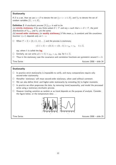
□ However treating variation as random or as trend depends on the purpose of analysis. Consider
the figure below, or the temperature data ...
Y(t)
0.0 0.5 1.0 1.5 2.0 2.5
Y(t)
0.0 0.5 1.0 1.5 2.0 2.5
0 20 40 60 80 100
t
0 2 4 6 8 10
t
Time Series Autumn 2008 – slide 25
12